4. Editing in a Spreadsheet

In This Chapter

• Renaming a spreadsheet

• Moving information

• Copying information

• Inserting and deleting rows and columns

• Hiding and redisplaying rows and columns

• Locking row and column titles onscreen

If you’ve been reading straight through, go take a break or you’ll fall asleep. Stand up and stretch, get some chocolate or caffeine (or both), and then come back and start learning about editing in a spreadsheet.

You’ll probably spend more time editing in a spreadsheet than you will doing any other activity, including producing reports or graphs. And, there are lots of ways to edit information in a spreadsheet. In Chapter 3, I showed you how to enter information into a cell, make corrections to that information, and fill a range with commonly used labels such as months. In this chapter, I’ll take things a step further.

In this chapter, you’ll learn how to how rename a spreadsheet, how to move and copy information from one location to another in a spreadsheet, how to insert, delete, hide, and redisplay columns and rows, and how to lock a set of rows and columns—usually the ones containing the titles of the information you are entering—onscreen so that you can always identify the information you’re viewing or entering.

Renaming a Spreadsheet

This isn’t a necessary technique, but it certainly makes working in a notebook easier when you use names instead of letters to identify spreadsheets. That way, you know exactly which sheet you need to click on when you want to switch to a different spreadsheet.

To rename a spreadsheet to something more meaningful than the alphabet letter Quattro Pro assigned to it, follow these steps:

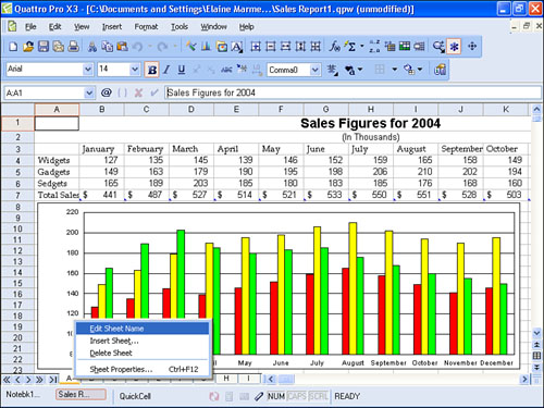
1. Right-click the tab of the spreadsheet you want to rename. Quattro Pro displays a shortcut menu (see Figure 4.1).
   

   Figure 4.1. Click Edit Sheet Name to make the spreadsheet name available so that you can change it.

   

2. Click Edit Sheet Name. Quattro Pro selects and displays the current name of the spreadsheet.
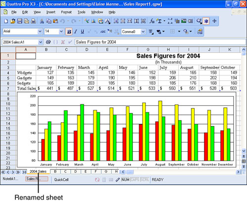
3. Type the new name you want to assign to the spreadsheet and press Enter.

Quattro Pro displays the sheet with the name that you assigned to it (see Figure 4.2).

Figure 4.2. You can assign meaningful names to spreadsheets in a notebook.

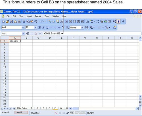
When you want to refer to formulas in that spreadsheet, you can use the name you assigned or you can use the alphabetic letter Quattro Pro originally assigned to the sheet. Regardless of which name you use, Quattro Pro displays the name you assigned to the sheet in the formula (see Figure 4.3).

Figure 4.3. When you refer to a different sheet in a formula, Quattro Pro uses the name you assigned to the sheet.

Moving Information

It happens—you enter information into the spreadsheet and then discover that you really don’t want it where you put it. Instead, you want it 5 columns to the right, or 10 rows down, or 5 columns to the right and 10 rows down. No, you don’t retype all the information; you move it.

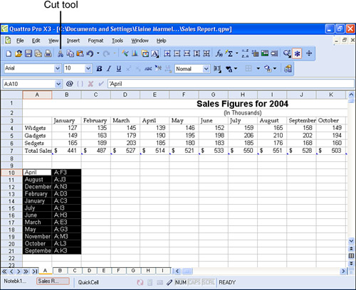
To move information, select the information and click the Cut button on the Notebook toolbar. The information disappears from the spreadsheet (see Figure 4.4).

Figure 4.4. Select the information that you want to move and click the Cut tool.

Then, move the cell selector to the cell that will act as the upper-left corner of the range you are moving and click the Paste tool on the Notebook toolbar. The information reappears in the new location (see Figure 4.5).

Figure 4.5. Select the upper-left corner of the new location and click the Paste tool.

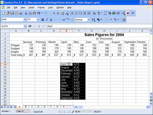
If you prefer and you don’t have a long distance to move, you can drag the information from one location to another. Select the range you want to move and then slide the mouse pointer over any edge of the selected range until the pointer changes to a four-headed arrow (see Figure 4.6). Once you see this pointer, you can drag the range to a new location.

Figure 4.6. When you see a four-headed arrow, you can drag a range to a new location.

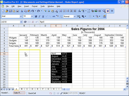
As you drag, the mouse pointer shape changes to a pointer with a square box attached, and Quattro Pro displays a yellow outline that represents the potential new location of the range (see Figure 4.7). When you release the mouse button, the yellow outline disappears and the selected information moves from its original location to the last location indicated by the yellow outline.

Figure 4.7. As you drag information to a new location, you see a yellow outline representing the potential location.

Copying Information

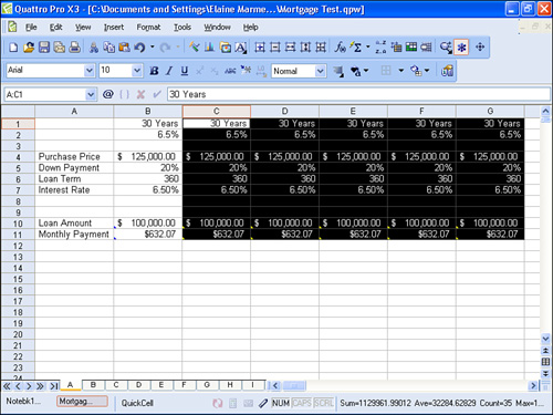
Suppose that you are getting ready to finance a new home and you want to compare several different scenarios involving varying down payments, loan terms, and interest rates. You set up a spreadsheet like the one shown in Figure 4.8 and then decide that you also want to calculate the Monthly Payment amount at 6.5% and 5.5% for 30 years and then all three interest rates (6%, 6.5%, and 5.5%) for 15 years. In this example, you could start by copying the values in Column B to Columns C through E and then simply edit the cells that need to change.

Figure 4.8. Select the cells that contain the information you want to copy.

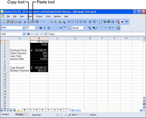
To copy the information, select all of the information that you want to copy—in this example, you need to select B1.B11—and then click the Copy tool on the Notebook toolbar.

Then, highlight the cells where you want the information to appear—in this example, I highlighted C1.E11—and click the Paste tool. Quattro Pro copies the information into the selected cells (see Figure 4.9). Click in any cell to cancel the selection. You can now change individual cells as needed.

Figure 4.9. Quattro Pro copies information into the selected range.

Inserting and Deleting Rows and Columns

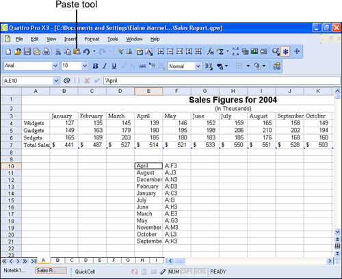
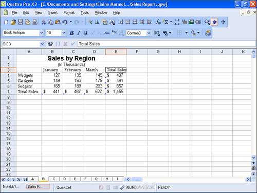
Sometimes, after setting up information in a spreadsheet, you realize that you left something out. For example, in the spreadsheet shown in Figure 4.10, suppose that you want to add information for April. Ideally, you’d like to insert a row or column to add the information. No problem; you can add a row or a column wherever you need.

Figure 4.10. You can insert a column to add April sales to this spreadsheet.

Follow these steps to insert a row or column:

1. Place the cell selector in the proper row or column to insert a row above the cell selector or a column to the left of the cell selector.
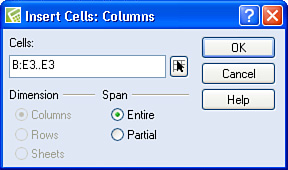
2. Open the Insert menu and click the appropriate command: Insert Row or Insert Column. When you select Insert Column, Quattro Pro displays the dialog box shown in Figure 4.11; only the title bar and the unavailable Dimension options are different when you select Insert Row.
   

   Figure 4.11. Use this dialog box to insert a column or row into a spreadsheet.

   

   

   When inserting a column, Quattro Pro inserts the column to the left of the column containing the cell selector. When you insert a row, Quattro Pro inserts the row above the row containing the cell selector. So make sure you initially position the cell selector properly to insert the row or column in the proper location.

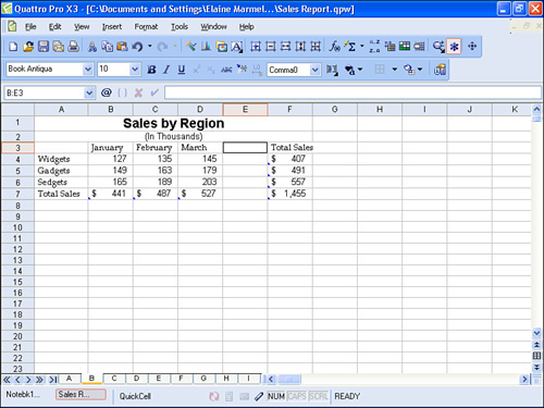
3. Click OK. Quattro Pro inserts a column to the left of the column containing the cell selector (see Figure 4.12); if you inserted a row, Quattro Pro inserts the row above the row containing the cell selector.
   

   Figure 4.12. Quattro Pro inserts columns to the left of the column containing the cell selector.

   

Hiding and Redisplaying Rows and Columns

There are occasions when you need to store a lot of information in a spreadsheet, but you want to look at only certain portions of it. For example, suppose you belong to a theater group that is putting on a play and you’ve been put in charge of tracking ticket sales. Suppose that your organization keeps track not only of the number of tickets sold but also the person who bought the ticket as well as the seat purchased, so that it can build a mailing list for the next production and perhaps offer prime seats to patrons who purchased more expensive tickets in the past. As an incentive, you might produce a list of names of those who paid for more expensive tickets.

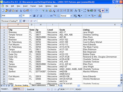
In such a scenario, you might set up a spreadsheet that looks something like the one in Figure 4.13 and Figure 4.14, where you track the purchaser’s address information, seat purchase, and listing. I’ve shown you the spreadsheet in two figures because you can’t see all of the information at one time.

Figure 4.13. Columns A through F of a large spreadsheet.

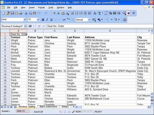
Figure 4.14. Columns F through K of the same large spreadsheet.

In spreadsheets like this one, there are times when you want to focus on certain information, and it is convenient to get the other information out of the way. You can hide rows or columns that you don’t want to view.

Suppose that you want to view the tickets purchased and you don’t care right now about address information. You can hide the columns containing the address information. Follow these steps to hide rows or columns:

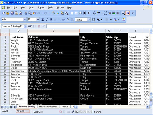
1. Select the rows or columns you want to hide; in Figure 4.15, I selected columns E through H.
   

   Figure 4.15. Select the rows or columns you want to hide.

   

   Tip

   

   You select an entire column by clicking the letter identifying the column; you select an entire row by clicking the number identifying the row. You select multiple columns by dragging across their column letters and multiple rows by dragging across their row numbers. You also can select noncontiguous rows or columns by holding down the Ctrl key as you click each row number or column letter.

2. Open the Format menu and click Selection Properties. Quattro Pro displays the Active Cells dialog box.
3. Click the Row/Column tab. This tab contains a section of Column Options and a section of Row Options.
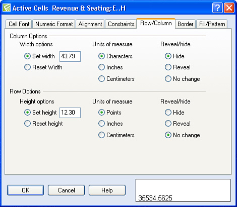
4. In the appropriate Column Options section or Row Options section, select the Hide option; in Figure 4.16, I selected the Hide option in the Column Options section.
   

   Figure 4.16. Select the Hide option in the appropriate section to hide the selected columns or rows.

   

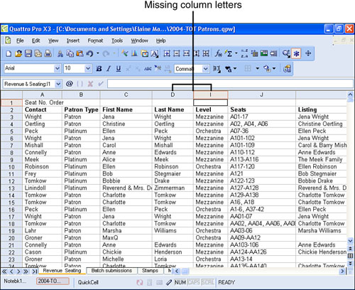
5. Click OK. Quattro Pro redisplays the spreadsheet, and the selected rows or columns no longer appear. In Figure 4.17, notice that the column headings go directly from Column D to Column I; the missing letters indicate that columns are hidden.
   

   Figure 4.17. The missing column letters provide you with a hint that columns are hidden.

   

To display hidden rows or columns again, select both rows or both columns on either side of the hidden rows or columns—in my example, I would select Column D and Column I, reopen the Active Cells dialog box, and, on the Row/Column tab, click the Reveal option in the appropriate Column Options or Row Options section.

Locking Row and Column Titles Onscreen

Again, suppose that you’re working in a spreadsheet containing a lot of data. You find, as you scroll around the spreadsheet, that you can’t remember what row or column you’re viewing. In cases like this one, lock the rows or columns containing labels onscreen so that you always view them. For example, suppose that I want to always view Row 2 as I scroll down the spreadsheet shown in Figure 4.18. I will lock Rows 1 and 2 onscreen so that they are always visible.

Figure 4.18. To lock rows or columns onscreen, place the cell selector in the top left cell of the spreadsheet that you want to be able to see when you scroll.

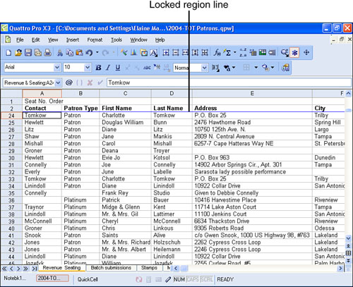
When you lock rows or columns, Quattro Pro locks the rows above the cell selector and the columns to the left of the cell selector. Therefore, position the cell selector in the cell below and to the right of the area that you want to lock onscreen. To lock Rows 1 and 2 without locking any columns, I placed the cell selector in cell A3. Then, open the View menu and click Locked Titles. Quattro Pro draws a blue line onscreen to separate the locked region from the region that will continue to scroll as you move around the spreadsheet. Notice, in Figure 4.19, the gap between Row 2 and Row 45; I scrolled down, but Rows 1 and 2 remain onscreen.

Figure 4.19. The blue line below row 2 indicates that rows 1 and 2 are permanent fixtures onscreen.

To unlock rows and columns, just open the View menu and click Locked Titles; the position of the cell selector doesn’t matter.