8. Formatting Notebooks

In This Chapter

• Using SpeedFormatting

• Aligning information

• Joining cells

• Applying numeric formatting to cells

• Setting row height

• Setting column width

• Swapping rows and columns

You can think of formatting as part of editing a spreadsheet, but you can compartmentalize formatting into the actions you take to change the appearance of your spreadsheet. In this chapter and the next chapter, you’ll read about most of the formatting you can apply to a Quattro Pro spreadsheet. In this chapter, I’ll introduce you to SpeedFormatting, a quick method to apply predesigned formatting to a spreadsheet. Then, we’ll explore some of the ways you can apply formatting on your own. Aligning information within cells, assigning numeric formats to cells, and setting row heights and column widths are some of the topics presented in this chapter.

Using SpeedFormatting

SpeedFormatting is a Quattro Pro tool that enables you to apply predefined formatting schemes to cells in your notebook. You select the formatting you want to apply, and Quattro Pro makes all the changes for you. SpeedFormatting is a quick and easy way to achieve elegant results.

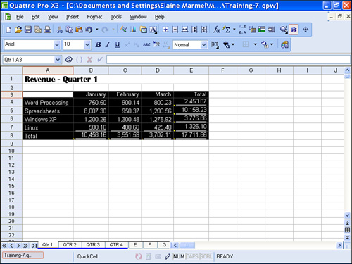
To apply a SpeedFormat, select the data in the spreadsheet that you want to format; in Figure 8.1, I selected everything but the title in cell A1.

Figure 8.1. Select the data in the spreadsheet that you want to format.

Then, open the Format menu and click SpeedFormat to select a predefined formatting scheme. Quattro Pro displays the SpeedFormat dialog box shown in Figure 8.2.

Figure 8.2. Use this dialog box to select a predefined set of formatting to apply to your spreadsheet.

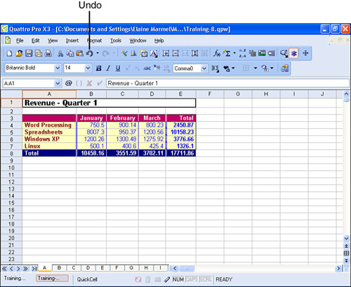
You can click each item in the Formats list to preview its appearance. When you find one you like, click OK. Quattro Pro applies the formatting to the selected cells. In Figure 8.3, I clicked outside the selection so that you can easily see the formatting.

Figure 8.3. Quattro Pro applies SpeedFormatting to the selected cells.

Aligning Information

SpeedFormatting doesn’t always accomplish everything you want, so you might choose to manually format your spreadsheet. One of the simplest techniques you can use to improve the appearance of your spreadsheet is to align information.

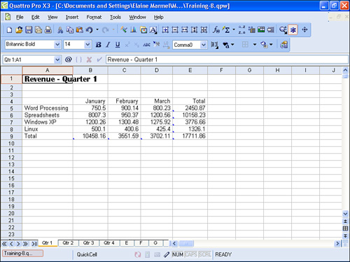
In Figure 8.4, Quattro Pro has assigned the default left alignment to text and the default right alignment to numbers. The appearance of the spreadsheet would be improved if the column headings (January, February, March, and Total) were either centered above the numbers or right-aligned. Because I prefer right-alignment, I’ll show you how to right-align the text in cells B4.E4; if you prefer centering, you can use the technique I describe to center the information.

Figure 8.4. If the column headings containing the month names were right-aligned over the data, the spreadsheet would look better.

To change the alignment of a cell or group of cells, select the cells you want to align (in this example, I selected B4.E4). Then, open the Format menu and click Selection Properties. In the Active Cells dialog box that appears (see Figure 8.5), click the Alignment tab.

Figure 8.5. Use this dialog box to set alignment for selected cells.

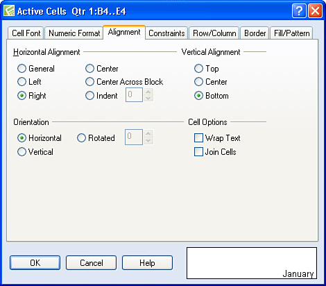
In the Horizontal Alignment section, click the Right option. Notice that you can preview the appearance of the proposed change in the lower-right corner of the dialog box. Click OK, and Quattro Pro applies the alignment formatting (see Figure 8.6).

Figure 8.6. The spreadsheet looks better after aligning the column titles to match the numeric alignment of the data in the columns.

Joining Cells

Joining cells enables you to use the space allotted to multiple cells as if they were one cell. Joining cells is really useful when you want to create a heading row for a spreadsheet or when you want to type explanatory text next to spreadsheet information to create a sidebar of information.

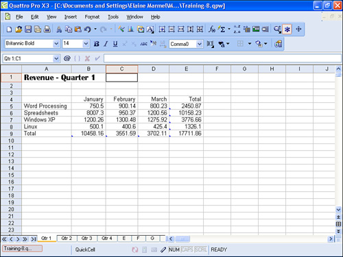
In Figure 8.7, I entered a spreadsheet title into cell A1. As you can see, the title spills over into the space occupied by cell B1. I’d really like to center the title over columns A through E, but, with the information in a single cell, that centering is difficult. I can simulate centering by moving the cell contents to cell C1. But, if I join cells A1.E1, Quattro Pro will treat them as one cell, and I can then easily center the title over columns A through E using the techniques described in the preceding section of this chapter.

Figure 8.7. In this spreadsheet, the title stored in cell A1 spills over into cell B1.

To join cells, follow these steps:

1. Select the cells you want to join; for this example, I selected A1.E1.
2. Open the Format menu and click Selection properties. Quattro Pro displays the Active Cells dialog box shown in Figure 8.8.
   

   Figure 8.8. Use this dialog box to join selected cells.

   

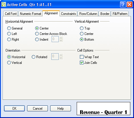
3. Click the Alignment tab.
4. In the Cell options area, place a check in the Join Cells check box.
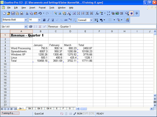
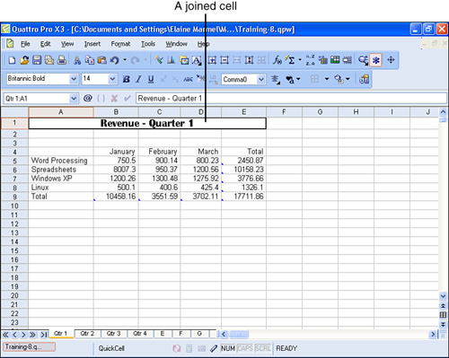
5. Click OK. Quattro Pro combines the selected cells into one cell. Compare Figure 8.9 to Figure 8.7; notice that the column dividers no longer appear in Figure 8.9.
   

   Figure 8.9. Because joined cells act as one cell, no column dividers appear in joined cells.

   

You can join cells in a row, in a column, or you can join a range that includes both rows and columns (useful for sidebar information). Whenever you join cells, the row or column dividers disappear from the joined range.

Applying Numeric Formatting to Cells

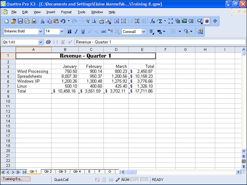
In Figure 8.9, the amounts that appear in cells B5.E9 don’t line up. In fact, they represent dollar amounts and, in some cases, you don’t even see two decimal places. Quattro Pro controls the appearance of numeric values using numeric formatting, and these numbers will be a lot easier to read if we apply numeric formatting to them.

Although all the values in the range are dollars, I’m going to apply Currency formatting to the totals and Number formatting to the rest of the range—cells B4.D7—because I believe the numbers will be easier to read. Readability is your top priority if you want your audience to seriously consider your spreadsheet work.

When you apply Currency formatting to numbers in Quattro Pro, Quattro Pro includes a dollar sign in the formatting. When you apply Number formatting, Quattro Pro does not include the dollar sign.

Follow these steps to apply numeric formats:

1. Select the cells you want to format; for this example, I’ll select cells B4.D7, the range to which I want to apply Number formatting.
2. Open the Format menu and click Selection Properties. Quattro Pro displays the Active Cells dialog box shown in Figure 8.10.
   

   Figure 8.10. Use the Numeric Format tab to select a format for numbers in your spreadsheet.

   

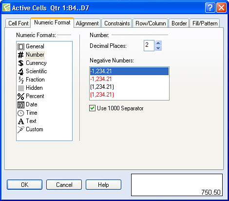
3. Click the Numeric Format tab.
4. In the Numeric Formats list, click an item. Quattro Pro displays information about the format to the right of the list; in the lower-right corner of the dialog box, you see a sample.
5. If you want to include a comma to separate thousand increments, check the Use 1000 Separator box.
6. Click OK. Quattro Pro applies the selected formatting.

To apply Currency formatting to the totals, I selected the range B8.E8 and E4.E8 simultaneously. Then, I repeated steps 2 through 6, selecting Currency in step 4. The Currency format allows you to use Accounting alignment, which adds space between the dollar sign and the first digit of the number. After applying both numeric formats, the spreadsheet looks like the one shown in Figure 8.11.

Figure 8.11. Cells B5.D8 use Number formatting, and cells B9.E9 and E5.E8 use Currency formatting with Accounting alignment.

Setting Row Height and Column Width

You can adjust the height of a row or the width of a column to improve the appearance and readability of a spreadsheet. To adjust either row height or column width, you can drag or you can use the Active Cells dialog box.

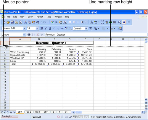
To adjust row height, move the mouse pointer into the row number area at the bottom of the row number that you want to adjust (see Figure 8.12). The mouse pointer shape changes to a pair of arrows pointing up and down. Drag down to increase the height of the row; drag up to reduce the height of the row. As you drag, a dotted line appears, marking the current height of the row.

Figure 8.12. Drag down to increase row height or up to reduce row height.

You can use the exact same technique to widen or narrow a column. Move the mouse pointer into the column letter area to the right side of the column that you want to make narrower or wider. Drag to the right to widen the column; drag to the left to make the column narrower.

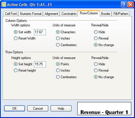
If you prefer to be more precise, place the cell pointer in any cell of the row or column you want to adjust. Then, open the Format menu and click Selection Properties. In the Active Cells dialog box, click the Row/Column tab (see Figure 8.13). In the Column Options section, type a number for the width of the column containing the selected cell in the Set Width box. In the Units of Measure column, select Characters, Inches, or Centimeters. To adjust row height, repeat the process in the Row Options section of the tab, typing the height in the Set Height box.

Figure 8.13. You can set row height or column width precisely using the Active Cells dialog box.

Swapping Rows and Columns

Occasionally, after setting up a spreadsheet, you might decide that the spreadsheet would work much better if you had the rows where the columns were and the columns where the rows were. Using Quattro Pro’s Transpose command, you can swap rows and columns quickly. There are two possible drawbacks to using the Transpose command:

• Any formulas in cells that you swap will not work. You’ll have to redo formulas in the transposed range.

• You cannot transpose data into the same range that contained the data originally. If you want the data to ultimately appear in the location where the original data appeared, transpose it outside the original range and then delete the extra rows and columns containing the original data. For help deleting rows and columns, see “Inserting and Deleting Rows and Columns” in Chapter 4, “Editing in a Spreadsheet.”

To transpose a range of rows and columns, follow these steps:

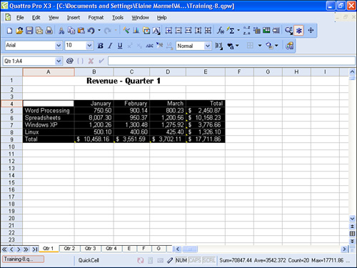
1. Select the rows and columns containing the data you want to swap; in Figure 8.14, I selected A4.E9.
   

   Figure 8.14. Select the data you want to swap.

   

2. Open the Tools menu, point to Numeric Tools, and click Transpose. Quattro Pro displays the Transpose Cells dialog box (see Figure 8.15).
   

   Figure 8.15. Use this dialog box to identify the range to transpose and the new location for the transposed range.

   

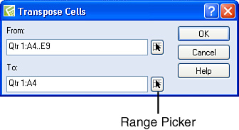
3. Click the Ranger Picker button in the To box. Quattro Pro collapses the Transpose Cells dialog box and allows you to select a new location for the transposed data.
4. Click any blank cell (in this example, I selected cell A13) and then click the Maximize button of the Transpose Cells dialog box.
5. Click OK. Quattro Pro displays the transposed data (see Figure 8.16).
   

   Figure 8.16. The transposed data begins in the cell you selected in the Transpose Cells dialog box.

   

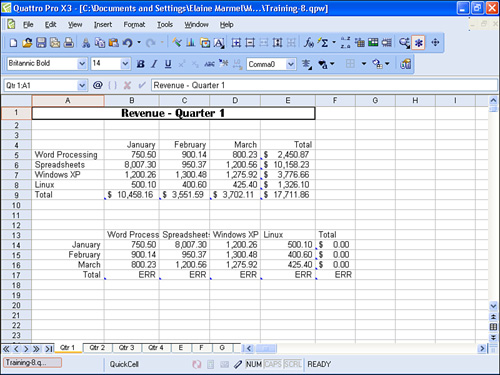
Notice that the formulas do not display correctly. Delete the contents of the cells containing the formulas and re-create the formulas. See Chapter 10, “Working with Calculations,” for help with spreadsheet calculations.

Also notice that Quattro Pro maintained the formatting of the transposed cells; you’ll probably want to reformat the transposed cells using the techniques described in this chapter and the next chapter.