
Chapter 11
Operating Decisions
This chapter introduces the operations function: the fulfilment of a customer order following the marketing function. We consider operations through the value chain and contrast the different operating decisions faced by manufacturing and service businesses. Several operational decisions are considered, in particular capacity utilization, the cost of spare capacity and the product/service mix under capacity constraints. Relevant costs are considered in relation to the make versus buy decision, equipment replacement and the relevant cost of materials. The cost of quality and environmental costs are also introduced.
The operations function
Operations is the function that produces the goods or services to satisfy demand from customers. This function, interpreted broadly, includes all aspects of purchasing, manufacturing, distribution and logistics, whatever those activities may be called in particular industries. While purchasing and logistics may be common to all industries, manufacturing will only be relevant to a manufacturing business. There will also be different emphases such as distribution for a retail business and the separation of ‘front office’ (or customer-facing) functions from ‘back office’ (or support) functions for a service business or financial institution.
Irrespective of whether the business is in manufacturing, retailing or services, we can consider operations as the all-encompassing processes that produce the goods or services that satisfy customer demand. In simple terms, operations is concerned with the conversion process between resources (materials, facilities and equipment, people) and the products/services that are sold to customers. There are four aspects of the operations function: quality, speed, dependability and flexibility (Slack et al., 1995). Each of these has cost implications and the lower the cost of producing goods and services, the lower can be the price to the customer, or the more profit may be retained by the business.
A useful analytical tool for understanding the conversion process is the value chain developed by Porter (1985) and shown in Figure 11.1. According to Porter every business is:
Figure 11.1 Porter’s value chain.
Source: Reprinted from Porter, M. E. (1985). Competitive Advantage: Creating and Sustaining Superior Performance. New York: Free Press.

a collection of activities that are performed to design, produce, market, deliver, and support its product . . . A firm’s value chain and the way it performs individual activities are a reflection of its history, its strategy, its approach to implementing its strategy, and the underlying economics of the activities themselves (Porter, 1985, p. 36).
Porter separated the value chain into primary and secondary activities. Primary activities commence with the upstream activities of research and development, product design and sourcing (which Porter calls ‘inbound logistics’), the production and distribution functions (‘operations’ and ‘outbound logistics’) and the downstream activities of marketing and after-sales customer service. This approach has similarities to the business process re-engineering approach of Hammer and Champy (1993, p. 32). Their emphasis on processes was on ‘a collection of activities that takes one or more kinds of input and creates an output that is of value to the customer’ (p. 35).
Accounting systems categorize costs through the hierarchical organization structure and line items (see Chapter 3) such as salaries and wages, rental and electricity. Porter argued that costs should be assigned to the value chain but that accounting systems can get in the way of analysing those costs. Traditional accounting systems ‘may obscure the underlying activities a firm performs’ (Porter, 1985). For many management decisions, far better information would be available from the categorization of costs in terms of value activities that are technologically and strategically distinct. This idea is part of the business process approach introduced in Chapter 9.
Porter developed the notion of cost drivers, which he defined as the structural factors that influence the cost of an activity and are ‘more or less’ under the control of the business. He proposed that the cost drivers of each value activity be analysed to enable comparisons with competitor value chains (we consider this further in Chapter 18). This would result in the relative cost position of the business being improved by better control of the cost drivers or by reconfiguring the value chain, while maintaining a differentiated product.
The value chain as a collection of inter-related business processes is a useful concept to understand businesses that produce either goods or services. Each element of the value chain contributes to the price a customer is willing to pay, but also attracts costs. As we saw with Porter’s views on competitive strategy in Chapter 10, accounting systems should provide cost and profitability information that supports the businesses operations strategy. This strategy will vary considerably depending on the type of business.
We first consider the role of operations in manufacturing and service industries. In describing operations throughout this book, we will use the term production to refer to either goods or services and use manufacturing where we specifically refer to the conversion of raw materials into finished goods.
Managing operations – manufacturing
A distinguishing feature between the sale of goods and services is the need for inventory or stock in the sale of goods. This topic was covered in detail in Chapter 8. Inventory enables the timing difference between production capacity and customer demand to be smoothed. This is of course not possible in the supply of services.
Manufacturing firms purchase raw materials (unprocessed goods) and undertake the conversion process through the application of labour, machinery and know-how to manufacture finished goods. The finished goods are then available to be sold to customers. There are actually three types of inventory in this example: raw materials, finished goods and work-in-progress. Work-in-progress consists of goods that have begun but have not yet completed the conversion process.
There are different types of manufacturing and it is important to differentiate these production techniques as they lead to different costing methods:
- Custom: unique, custom products produced singly, e.g. a building.
- Batch: a quantity of the same goods produced at the same time (often called a production run), e.g. textbooks.
- Continuous: products produced in a continuous production process, e.g. oil and chemicals.
For continuous production processes, a process costing system is used. For custom and batch manufacture, costs are collected through a job costing system. In a manufacturing business the materials are identified by a bill of materials, a list of all the components that go to make up the completed project, and a routing, a list of the labour or machine-processing steps and times for the conversion process. To each of these costs overhead is allocated to cover the manufacturing costs that are not included in either the bill of materials or the routing (overhead will be covered in Chapter 13). This chapter will assume a job costing system is used, but readers interested in process costing are encouraged to read Chapter 8.
The bill of materials and routing contain standard quantities of raw material and labour time for a unit (or batch) of product. Standard quantities are the expected raw materials quantities, based on past and current experience and planned improvements in product design, purchasing and methods of production. Standard costs are the standard quantities of raw materials or labour times multiplied by the current and anticipated purchase prices for materials and the labour rates of pay. The standard cost is therefore a budget cost for a unit or batch of a product. As actual costs are not known for some time after the end of the accounting period, standard costs are generally used for decision making. Standard costs are usually expressed per unit.
The manufacturing process and its relationship to accounting can be seen in Figure 11.2. When a custom product is completed, the accumulated cost of materials, labour and overhead is the cost of that custom product. For a batch the total job cost is divided by the number of units produced. In process costing, at the end of the accounting period the total costs are divided by the volume produced to give a cost per unit of volume. The actual cost per unit can be compared to the budget or standard cost per unit. Any variation needs to be investigated and corrective action taken (we explain this in Chapter 17).
Figure 11.2 The manufacturing process and its relationship to standard costs.
The distinction between custom and batch is not always clear. Some products are produced on an assembly line as a batch of similar units but with some customization, because technology allows each unit to be unique. For example, motor vehicles are assembled as ‘batches of one’, since technology facilitates the sequencing of different specifications for each vehicle along a common production line. Within the same vehicle model, different colours, transmissions (manual or automatic), steering (right-hand or left-hand drive) and so on can all be accommodated.
Any manufacturing operation involves a number of sequential activities that need to be scheduled so that materials arrive at the appropriate time at the correct stage of production and labour is available to carry out the required process. Organizations that aim to have material arrive in production without holding buffer stocks are said to operate a just-in-time (JIT) manufacturing system. A case study of an automotive JIT can be found in Berry and Collier (2007).
Most manufacturing processes require an element of set-up or make-ready time, during which equipment settings are made to meet the specifications of the next production run (a custom product or batch). These settings may be made by manual labour or by computer through CNC (computer numerical control) technology. These investments involve substantial costs that need to be justified by an increased volume of production or by efficiencies that reduce production costs (we discuss investment decisions in Chapter 14). Set-up costs are built into the cost of production and are spread over the number of units in a batch.
The accumulated cost of materials, labour and overhead is the cost of a custom product or a batch of the same products. We can illustrate this with the example of a production run or batch of textbooks. The standard cost for the printing of 5,000 copies of a textbook is as follows:
| Raw materials (paper, ink, etc.) from bill of materials | 12,000 |
| Machine set-up time (paper size, ink colours, etc.) | 2,000 |
| Labour time for printing (from labour routing) | 18,000 |
| Overhead allocated | 10,000 |
| Total job cost | €42,000 |
For a batch the total job cost is divided by the number of units produced (e.g. the number of copies of the textbook) to give a cost per unit (cost per textbook). In this illustration, the standard cost per textbook is €8.40 (€42,000/5,000 copies).
The most important difference between manufacturing goods and providing services is the absence of raw materials from the conversion process. Services are more concerned with the application of human knowledge, skill and experience, although often services can involve substantial investments in capital equipment, as the next section illustrates.
Managing operations – services
Service or knowledge-based industries have increasingly become the focus of Western economies. Fitzgerald et al. (1991) identified four key differences between products and services: intangibility, heterogeneity, simultaneity and perishability. Services are intangible rather than physical and are often delivered in a ‘bundle’ such that customers may value different aspects of the service. Services involving high labour content are heterogeneous, i.e. the consistency of the service may vary significantly. The production and consumption of services are simultaneous so that services cannot be inspected before they are delivered. Services are also perishable, so that unlike physical goods, there can be no inventory of services that have been provided but remain unsold.
Fitzgerald et al. also identified three different service types. Professional services are ‘front office’, people based, involving discretion and the customization of services to meet customer needs in which the process is more important than the service itself. Examples given by Fitzgerald et al. include professional firms such as solicitors, auditors and management consultants. Mass services involve limited contact time by staff and little customization, with services equipment based and product oriented with an emphasis on the ‘back office’ and little autonomy. Examples here are rail transport, airports and mass retailing. The third type of service is the service shop, a mixture of the other two extremes with emphasis on front and back office, people and equipment and product and process. Examples of service shops are banking and hotels.
Fitzgerald et al. emphasized how cost traceability differed between each of these service types. Their research found that many service companies did not try to cost individual services accurately either for price-setting or profitability analysis, except for the time-recording practices of professional service firms. In mass services and service shops there were:
multiple, heterogeneous and joint, inseparable services, compounded by the fact that individual customers may consume different mixes of services and may take different routes through the service process (p. 24).
In these two categories of services, costs were controlled not by collecting the costs of each service but through responsibility centres (this topic is covered in more detail in Chapter 15). Following this argument, we can see that when you travel by rail, there is no calculation of the cost of your rail journey, or the cost of your hotel room. Nevertheless, these organizations must still understand their cost structures and ensure that the prices they charge, in the aggregate, cover all their costs and generate a profit.
Slack et al. (1995) contrasted types of service provision with types of manufacturing and used a matrix of low volume/high variety and high volume/low variety, comparing:
- professional service with customized or batch manufacturing (i.e. job costing);
- mass service with continuous manufacture (i.e. process costing); and
- service shop with a batch-type process (i.e. job costing).
Accounting information has an important part to play in operational decisions. Typical questions that may arise include:
- What is the cost of spare capacity?
- What product/service mix should be produced where there are capacity constraints?
- What are the costs that are relevant for particular operational decisions?
This chapter considers each of these in turn.
Accounting for the cost of spare capacity
Production resources (material, facilities/equipment and people) allocated to the process of supplying goods and services provide a capacity. The utilization of that capacity is a crucial performance driver for businesses, as the investment in capacity often involves substantial outlays of funds that need to be recovered by utilizing that capacity fully in the production of products/services. Capacity may also be a limitation for the production and distribution of goods and services where market demand exceeds capacity. So, for example, an airline will want to fully utilize all its seats on every flight. A factory will want to work its assets harder and maximize production volume. A professional services firm will want its professionals working all the time on behalf of clients.
A weakness of traditional accounting is that it equates the cost of using resources with the cost of supplying resources because financial statements reveal only the cost of resources supplied, not whether any of those resources were wasted through under-utilization. Activity-based costing (which is described further in Chapter 13) has as a central focus the identification and elimination of unused capacity. According to Kaplan and Cooper (1998), there are two ways in which unused capacity can be eliminated:
Identifying the difference between the cost of resources supplied and the cost of resources used as the cost of the unused capacity enables management to take appropriate corrective action.
![]()
An example illustrates this.
Ten staff, each costing $30,000 per year, deliver banking services where the cost driver (the cause of the activity) is the number of banking transactions.
Assuming that each member of staff can process 2,000 transactions per annum, the cost of resources supplied is $300,000 (10 × $30,000) and the capacity number of transactions is 20,000 (10 × 2,000). The standard cost per transaction would be $15 ($300,000/20,000 transactions).
If in fact 18,000 transactions were carried out in the year, the cost of resources used would be $270,000 (18,000 @ $15) and the cost of unused capacity would be $30,000 (2,000 @ $15, or $300,000 resources supplied minus $270,000 resources used). If the cost of resources used is equated with the cost of resources supplied, the actual transaction cost becomes $16.67 ($300,000/18,000 transactions) and the cost of unused capacity is not identified separately. This is a weakness of traditional accounting systems.
Although there can be no carry forward of an ‘inventory’ of unused capacity in a service delivery function, management information is more meaningful if the standard cost is maintained at $15 and the cost of spare capacity is identified separately. Management action can then be taken to reduce the cost of spare capacity to zero, either by increasing the volume of business or reducing the capacity (i.e. the number of staff).
A different situation arises where there is insufficient capacity and management needs to make choices between alternative product/services.
Capacity utilization and product mix
Where demand exceeds the capacity of the business to produce goods or deliver services as a result of scarce resources (whether that is space, equipment, materials or staff), the scarce resource is the limiting factor. A business will want to maximize its profitability by selecting the optimum product/service mix. The product/service mix is the mix of products or services that will be sold by the business (we referred to this as the sales mix in Chapter 10 in relation to marketing, but we use product/service mix here to refer to the production process), each of which may have different selling prices and costs. It is therefore necessary, where demand exceeds capacity, to rank the products/services with the highest contributions, per unit of the limiting factor (i.e. the scarce resource).
For example, Beaufort Accessories makes three parts (F, G and H) for a motor vehicle, each with different selling prices and variable costs and requiring a different number of machining hours. These are shown in Table 11.1. However, Beaufort has an overall capacity limitation of 10,000 machine hours.
Table 11.1 Beaufort Accessories cost information.

The first step is to identify the ranking of the products by calculating the contribution per unit of the limiting factor (machine hours in this case) for each product. This is shown in Table 11.2.
Table 11.2 Beaufort Accessories – product ranking based on contribution.
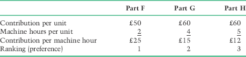
Although both Part G and Part H have higher contributions per unit, the contribution per machine hour (the unit of limited capacity) is higher for Part F. Profitability will be maximized by using the limited capacity to produce as many Part Fs as can be sold, followed by Part Gs. Based on this ranking, the available production capacity can be allocated as follows:
| Production | Contribution |
| 2,000 of Part F @ 2 hours = 4,000 hours. 2,000 @ £50 per unit = £100,000 | 2,000 @ £50 per unit = £100,000 |
| Based on the capacity limitation of 10,000 hours, there are 6,000 hours remaining, so Beaufort can produce 3/4 of the demand for Part G (6,000 hours available/8,000 hours to meet demand) equivalent to 1,500 units of part G (3/4 of 2,000 units). | |
| 1,500 of Part G @ 4 hours = 6,000 hours | 1,500 @ £60 per unit = £90,000 |
| Maximum contribution | £190,000 |
| There is no available capacity for Part H |
This example shows that managers should not be swayed by simple measures of sales revenue (the highest price) or even the highest contribution per unit of product/service (as we saw in Chapter 10) but should focus on optimizing the use of limited production capacity by comparing the contribution earned from the use of the available production capacity. However, there is an alternative to this approach to capacity utilization.
Theory of Constraints
A different approach to limited capacity was developed by Goldratt and Cox (1986), who focused on the existence of bottlenecks in production and the need to maximize volume through the bottleneck (throughput) rather than through production capacity as a whole. This is because a bottleneck resource can limit the overall production volume of a business. Goldratt and Cox developed the Theory of Constraints (ToC), under which only three aspects of performance are important: throughput contribution, operating expense and inventory. Throughput contribution is defined as sales revenue less the cost of materials:
![]()
Goldratt and Cox considered all costs other than materials as fixed and independent of customers and products, so operating expenses included all costs except materials. Labour to them, at least in the short term, was a fixed cost. They emphasized the importance of maximizing throughput while holding constant or reducing operating expenses and inventory. Goldratt and Cox also recognized that there was little point in maximizing non-bottleneck resources if this leads to an inability to produce at the bottlenecks.
Applying the Theory of Constraints to the Beaufort Accessories example and assuming that machine hours are the bottleneck resource (in practice, the bottleneck resource may be a different measure), Table 11.3 shows the throughput ranking. Under the Theory of Constraints, Part F retains the highest ranking but Part H has a higher return per unit of the bottleneck resource than Part G after deducting only the variable cost of materials. This is a different ranking to the previous method, which used the contribution after deducting all variable costs. The difference is due to the treatment of variable costs other than materials.
Table 11.3 Beaufort Accessories – product ranking based on throughput.
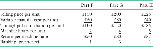
Which is the preferred method? Both have value. As in many situations using management accounting information to make decisions, different assumptions can lead to different decisions. It is important to be explicit about your assumptions but to make assumptions that are most realistic in terms of the unique conditions that apply to each business. So a business with a lot of contract staff whose wage costs could readily be avoided might prefer the first approach treating labour costs as variable costs. A business which has long-term commitments to permanent staff will pay those staff irrespective, and so the throughput approach may lead to more meaningful information.
This leads us to think about the issue of when costs are relevant to a particular decision at a particular point in time.
Operating decisions: relevant costs
Operating decisions imply an understanding of costs, but not necessarily those costs that are defined by accountants and are recorded in the company’s accounting system. We have already seen in Chapter 10 the distinction between avoidable and unavoidable costs. This brings us to the notion of relevant costs. Relevant costs are those costs that are relevant to a particular decision. Relevant costs are the future, incremental cash flows that result from a decision. Relevant costs specifically do not include sunk costs, i.e. costs that have been incurred in the past, as nothing we can do can change those earlier decisions. Relevant costs are avoidable costs because, by taking a particular decision, we can avoid the cost. Unavoidable costs are not relevant because, irrespective of what our decision is, we will still incur those costs. Relevant costs may, however, be opportunity costs. An opportunity cost is not a cost that is paid out in cash. It is the loss of a future cash flow that takes place as a result of making a particular decision.
Three examples illustrate how relevant costs can be applied:
- make versus buy decisions;
- equipment replacement decisions;
- pricing decisions using the cost of materials.
Make versus buy?
A concern with subcontracting or outsourcing has dominated Western business in recent years as the cost of producing goods and services in-house has been increasingly compared with the cost of purchasing goods on the open market, which has often entailed a shift to off-shore locations. The make versus buy decision should be based on which alternative is less costly on a relevant cost basis, that is, taking into account only future, incremental cash flows.
For example, the costs of in-house production of a computer processing service that averages 10,000 transactions per month are calculated as €25,000 per month. This comprises €0.50 per transaction for stationery and €2 per transaction for labour. In addition, there is a €10,000 charge from head office as the share of the depreciation charge for computer equipment. An independent computer bureau has tendered a fixed price of €20,000 per month.
Based on this information, we judge that stationery and labour costs are variable costs that are both avoidable if processing is outsourced. The depreciation charge will remain a cost to the business irrespective of the outsourcing decision. It is therefore unavoidable. The fixed outsourcing cost will only be incurred if outsourcing takes place.
The total costs for each alternative can be compared as shown in Table 11.4. The relevant costs for the alternatives are shown in Table 11.5. In Table 11.5 the €10,000 share of depreciation costs is not shown as it is not relevant to the decision because it is unavoidable.
Table 11.4 Total costs – make versus buy.
| Cost to make | Cost to buy | |
| Stationery | 5,000 | |
| 10,000 @ €0.50 | ||
| Labour | 20,000 | |
| 10,000 @ €2 | ||
| Share of depreciation costs | 10,000 | 10,000 |
| Outsourcing cost | 0 | 20,000 |
| Total relevant cost | €35,000 | €30,000 |
Table 11.5 Relevant costs – make versus buy.
| Relevant cost to make | Relevant cost to buy | |
| Stationery | 5,000 | |
| 10,000 @ €0.50 | ||
| Labour | 20,000 | |
| 10,000 @ €2 | ||
| Outsourcing cost | 0 | 20,000 |
| Total relevant cost | €25,000 | €20,000 |
Both Table 11.4 and 11.5 show the same information, but the presentation is different. In either case there would be a €5,000 per month saving by outsourcing the computer processing service (total costs of €30,000 compared to €35,000; or relevant costs of €20,000 compared to €25,000).
Equipment replacement
A further example of the use of relevant costs is the decision to replace plant and equipment. Once again, the concern is with future incremental cash flows, not with historical or sunk costs or with non-cash expenses such as depreciation. While the following illustration is unlikely to occur in practice, it does illustrate the different perspective that relevant costs brings to a decision.
Mammoth Hotel Company replaced its kitchen one year ago at a cost of $120,000. The kitchen was to be depreciated over five years, although it will still be operational after that time. The hotel manager wishes to expand the dining facility and needs a larger kitchen with additional capacity. A new kitchen will cost $150,000, but the kitchen equipment supplier is prepared to offer $25,000 as a trade-in for the old kitchen. The new kitchen will ensure that the dining facility earns additional income of $25,000 for each of the next five years.
The existing kitchen incurs operating costs of $40,000 per year. Due to labour-saving technology, operating costs, even with additional dining, will fall to $30,000 per year if the new kitchen is bought. These figures are shown in Table 11.6. On a relevant cost basis, the difference between retaining the old kitchen and buying the new kitchen is a saving of $50,000 cash flow over five years. On this basis, it makes sense to buy the new kitchen.
Table 11.6 Relevant costs – equipment replacement.
| Retain old kitchen | Buy new kitchen | |
| Purchase price of new kitchen | −$150,000 | |
| Trade-in value of old kitchen | +$25,000 | |
| Operating costs | ||
| $40,000 p.a. × 5 years | −$200,000 | |
| $30,000 p.a. × 5 years | −$150,000 | |
| Additional income from dining of | +$125,000 | |
| $25,000 p.a. × 5 years | _____ | _____ |
| Total relevant cost | −$200,000 | −$150,000 |
However, we cannot ignore the implications of this decision on the financial statements. The original kitchen cost has been written down to $96,000 (cost of $120,000 less one year’s depreciation at 20% or $24,000). The original capital cost is a sunk cost and is therefore irrelevant to a future decision. The loss on sale of $71,000 ($96,000 written-down value – $25,000 trade-in) will affect the hotel’s reported profit, but it is not a future incremental cash flow and is therefore irrelevant to the decision. But such a loss reported in the Statement of Comprehensive Income may not present the company in the best possible light to shareholders. There is a tension between a decision based on future incremental cash flows and how that decision (although positive for future profitability) will be seen in relation to past performance. A result of this tension could be that managers do not take advantage of this opportunity and so do not generate additional shareholder wealth because of the negative perceptions such a decision may leave in the year in which the old kitchen is written off. The political aspects of such a decision were discussed in Chapter 5. Other aspects of capital expenditure decisions are explained in Chapter 14.
Relevant cost of materials
As the definition of relevant cost is the future incremental cash flow, it follows that the relevant cost of materials is not the historical (or sunk) cost but the replacement cost of the materials. This is particularly important in pricing decisions for special orders (for an example see Chapter 10). It is irrelevant whether or not those materials are held in inventory, and they may well be used to fulfil a special order, but the relevant cost remains the future, incremental cash flow. In most cases this will be the replacement cost for the materials, but in some circumstances it may be the opportunity cost where the materials have only scrap value or an alternative use. The relevant cost of materials can be summarized as follows:
- If the material is purchased specifically for the special order, the relevant cost is the replacement price.
- If the material is already in stock and is used regularly in the business, the relevant cost is the replacement price.
- If the material is already in stock but is surplus to business requirements (other than for this special order), the relevant cost is the opportunity cost, which may be its scrap value or its value in any alternative use.
Stanford Potteries Ltd has been approached by a customer who wants to place a special order and is willing to pay £16,000. The order requires the materials shown in Table 11.7.
Table 11.7 Material requirements.
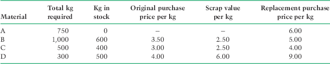
In Table 11.7, the ‘original purchase price’ column is the cost of materials as would be shown in the company’s accounting system when the stock was purchased. The ‘replacement purchase price’ column is the amount that is charged by suppliers for any stock to be purchased currently.
For this special order, Material A would have to be purchased specifically for this order. Material B is used regularly and any inventory used for this order would have to be replaced. Material C is surplus to requirements and has no alternative use. Material D is also surplus to requirements but can be relabelled and used as a substitute for Material E without additional cost. Material E, although not required for this order, is in regular use and currently costs £8.00 per kg, but is not in stock. The calculation of relevant material costs is shown in Table 11.8.
Table 11.8 Relevant cost of materials.
| Material | Relevant cost £ | |
| A | 750 kg @ £6 (replacement price) | 4,500 |
| B | 1,000 kg @ £5 (replacement price) | 5,000 |
| C | 400 kg @ £2.50 (opportunity cost of scrap value) | 1,000 |
| 100 kg @ £4 (replacement price) | 400 | |
| D | 300 kg @ £6 (opportunity cost of scrap value) | 1,800 |
| or | ||
| 300 kg @ £8 (substitute for Material E) | 2,400 | |
| Total relevant cost of materials | 13,300 | |
| Revenue from special order | 16,000 | |
| Future, incremental cash flow gain | 2,700 |
As a result of the above, Stanford Potteries would accept the special order because the additional income exceeds the relevant cost of materials. In the case of A, the material is purchased at the replacement purchase price. For Material B, even though some inventory is held at a lower cost price, it is used regularly and has to be replaced at the current purchase price. It is important to note that the 600 kg of Material B in stock may physically be used, but will need to be replaced – remember it is the future incremental cash flow of £5 and not the sunk cost of £3.50 that is relevant to this decision.
For Material C, the 400 kg in inventory has no other value than scrap, so the relevant cost is the opportunity cost (i.e. the loss of generating scrap value of 400 kg @ £2.50) by using Material C for this order. The 100 kg of Material C not in inventory has to be purchased at the replacement purchase price. For Material D, the opportunity cost is either the scrap value or the saving made by using Material D as a substitute for Material E. The question here is: ‘What would the company do in the absence of this special order?’ As the substitution value is higher, this is what Stanford would do in the absence of this particular order. Therefore, the opportunity cost of Material D is the loss of the ability to substitute for Material E.
Remember that the relevant cost of materials in Table 11.8 is not the same as the cost that would be recorded in Stanford’s accounting system. Table 11.9 shows how the accounting system would record the cost of materials. It would (as explained in Chapter 8) cost anything used from inventory using the original purchase price, and any inventory purchased would be at the replacement price. Table 11.9 shows the materials cost as £11,400 – somewhat different to the relevant cost of materials of £13,300 shown in Table 11.8.
Table 11.9 Comparison of relevant cost and accounting cost of materials.
| Material | Accounting cost £ | |
| A | 750 kg @ £6 | 4,500 |
| B | 600 kg in stock @ £3.50 400 kg to be purchased @ £5 | 2,100 |
| 400 kg to be purchased @ £5 | 2,000 | |
| C | 400 kg in stock @ £3 | 1,200 |
| 100 kg to be purchased @ £4 | 400 | |
| D | 300 kg in stock @ £4 | 1,200 |
| Total | £11,400 |
Relevant costs are defined differently – as future, incremental cash flows – to accounting costs which are defined in actual, historic terms. Both provide useful, but different, information on which to make judgements. A relevant cost approach helps to understand the impact, in cash flow terms, of future decisions. Accounting costs are important signals of past performance, but can distort management decisions, which should be made in terms of whether a particular decision will improve shareholder value in the future.
Relevant costs are a useful tool in helping to make operational decisions. There other important aspects of costs that rarely appear in financial statements, and if they do so, are not often identifiable. Two particular types of cost are:
- costs of quality;
- environmental costs.
Total quality management and the cost of quality
One aspect of operational management that deserves particular attention is total quality management and the cost of quality. Total quality management (TQM) encompasses design, purchasing, operations, distribution, marketing and administration. A TQM approach emphasizes continuous improvement through a systematic approach to quality management that focuses on customer expectations, re-engineers business processes, ensures the quality of goods and services from suppliers, and ensures that all employees are committed to quality improvement. Standardization of processes ensures consistency, which may be documented in a quality management system such as ISO 9000.
TQM involves comprehensive measurement systems, often developed from statistical process control (SPC) approaches.
The Six Sigma approach, developed by Motorola, is a measure of standard deviation, i.e. how tightly clustered observations are around a mean (the average). Six Sigma aims to improve quality by removing defects and the causes of defects. It is well developed as a management tool in high-technology manufacturing organizations and is part of a performance measurement model called DMAIC, an acronym for Define, Measure, Analyse, Improve and Control. Quality will likely be a measure included in a Balanced Scorecard (see Chapter 4).
Not only is non-financial performance measurement crucial in TQM, but accounting has a significant role to play because of its ability to record and report the cost of quality and how cost influences, and is influenced by, continuous improvement in production processes.
Recognizing the cost of quality is important in terms of continuous improvement processes. The Chartered Institute of Management Accountants define the cost of quality as the difference between the actual costs of production, selling and after-sales service and the costs that would be incurred if there were no failures during production or usage of product/services. There are two broad categories of the cost of quality: conformance costs and non-conformance costs.
Conformance costs are those costs incurred to achieve the specified standard of quality and include prevention costs such as quality measurement and review, supplier review and quality training (i.e. the procedures required by an ISO 9000 quality management system). Costs of conformance also include the costs of inspection or testing to ensure that products or services actually meet the quality standard.
The costs of non-conformance include the cost of internal and external failure. Internal failure is where a fault is identified by the business before the product/service reaches the customer, typically evidenced by the cost of waste or rework. The cost of external failure is identified after the product/service is in the hands of the customer. Typical costs are warranty claims, discounts and replacement costs.
Identifying the cost of quality is important to the continuous improvement process, as substantial improvements to business performance can be achieved by investing in conformance and so avoiding the much larger costs usually associated with non-conformance.
Although SPC or Six Sigma based systems will measure quality performance, accounting systems rarely reflect the costs of prevention, inspection, internal and external failure costs, so the costs of quality tend to be buried in production costs as rework, waste and so on. This leads to the problem that the true cost of quality to a business is not known and therefore action to address the cause of quality problems may not be undertaken.
A similar situation arises in respect to environmental costs.
Environmental cost management
Of increasing importance to organizations are costs relating to environmental protection (including land, water and air pollution, waste treatment) and the costs of remedying problems caused during the production process. Environmental costs involve recognition of the importance of corporate social responsibility (see Chapter 7). International Standard ISO 14000 is an international standard on environmental management. Like ISO 9000 for quality, ISO 14000 provides a framework for the development of both the system and the supporting audit program and specifies a framework of control for an environmental management system against which an organization can be certified by a third party.
Environmental management accounting recognizes environmental costs for decision making, with the principles of measuring environmental costs being similar to those for measuring quality costs. Environmental management accounting is concerned with collecting, measuring and reporting costs about the environmental impact of an organization’s activities. As for quality management, these costs can be broken down into four types: prevention costs, to avoid environmental damage (e.g. the cost of equipment to reduce pollution and the training of employees); measurement costs, to determine the extent of the organization’s environmental impact (including testing, monitoring and external certification); internal failure costs, where remedial action has to be taken (e.g. cleaning up spillages or leakages, or employee health and safety-related damages); and external failure costs (e.g. penalties incurred for environmental damage).
As countries begin to develop carbon taxes or emissions trading schemes to reduce greenhouse gas emissions, environmental accounting is likely to increase in importance, not only in relation to external reporting and audit requirements, but also in how organizations take environment-related costs into consideration in their decision making.
For most organizations, as for continuous quality improvement, continuous environmental improvement is likely to result from an investment in preventive measures and measurement to enable corrective action, rather than in after-the-event remedying the cost of failure. Failure can involve substantial costs, both financial and reputational (e.g. the 2010 Deepwater Horizons explosion and oil spill in the Gulf of Mexico which severely damaged the reputation of BP).
Three case studies illustrate the main concepts identified in this chapter.
Table 11.10 Quality Printing Company – business performance trends.

Table 11.11 Quality Printing Company – analysis of business performance.

Table 11.12 Quality Printing Comapny – throughput contribution.
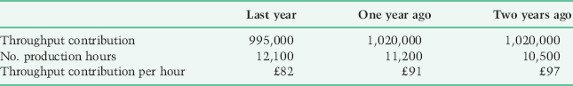
Table 11.13 Vehicle Parts Company.
| Existing machine | New CNC machine | |
| Original cost | €250,000 | €1,000,000 |
| Depreciation at 20% p.a. | fully written off | 200,000 |
| Available hours (2 shifts) | 1,920 | 1,920 |
| Set-up time | 35% | 5% |
| Running time | 65% | 95% |
| Available running hours | 1,248 | 1,824 |
| Hours per part | 0.5 | 0.35 |
| Production capacity (number of parts) | 2,496 | 5,211 |
| Market capacity | 2,500 | |
| € | € | |
| Depreciation cost per part | 0 | 80 |
| Material cost per part | 75 | 75 |
| Labour and other costs per part | 30 | 20 |
| Total cost per part | 105 | 175 |
| Mark-up 50% | 53 | 88 |
| Selling price | 158 | 263 |
| Maximum selling price | 158 | |
| Effective markdown on cost | −10% |
| Production labour $1.2 million – estimated 5% rework | $60,000 |
| Waste removal costs associated with poor quality production | 40,000 |
| Lost time due to injuries, legal costs and fines | 50,000 |
| Lost sales $400,000 at gross margin of 30% | $120,000 |
| Total | $270,000 |
Conclusion
Operations decisions are critical in satisfying customer demand. Understanding the cost of each element in the value chain is an important ingredient in making operational decisions and this includes an understanding of the difference between manufacturing and services costing, what constitutes the standard cost of a product or service and the cost of spare capacity. It is important that businesses maximize their existing production capacity through seeking out those products/services that generate the highest contribution per unit of the limiting production capacity. It is also important to distinguish historic costs derived from an accounting system from relevant costs for decision making (defined as future incremental cash flows). The identification of the cost of quality and environmental costs is also important in planning, decision making and control.
References
Berry, A. J. and Collier, P. M. (2007). Risk management in supply chains: processes, organisation for uncertainty and culture. International Journal of Risk Assessment and Management, 7(8), 1005–26.
Fitzgerald, L., Johnston, R., Brignall, S., Silvestro, R. and Voss, C. (1991). Performance Measurement in Service Businesses. London: Chartered Institute of Management Accountants.
Goldratt, E. M. and Cox, J. (1986). The Goal: A Process of Ongoing Improvement (Revd. edn). Croton-on-Hudson, NY: North River Press.
Hammer, M. and Champy, J. (1993). Reengineering the Corporation: A Manifesto for Business Revolution. London: Nicholas Brealey.
Kaplan, R. S. and Cooper, R. (1998). Cost and Effect: Using Integrated Cost Systems to Drive Profitability and Performance. Boston, MA: Harvard Business School Press.
Porter, M. E. (1985). Competitive Advantage: Creating and Sustaining Superior Performance. New York: Free Press.
Slack, N., Chambers, S., Harland, C., Harrison, A. and Johnston, R. (1995). Operations Management. London: Pitman Publishing.
| November | December | |
| Activity level in units | 5,000 | 10,000 |
| £ | £ | |
| Variable costs | 10,000 | ? |
| Fixed costs | 30,000 | ? |
| Semi-variable costs | 20,000 | ? |
| Total costs | 60,000 | 75,000 |
- variable costs;
- fixed costs;
- semi-variable costs.
| Product R | Product S | |
| € | € | |
| Selling price | 12 | 20 |
| Raw materials | 4 | 11 |
| Production labour hours | 2 | 4 |
| Machine hours | 4 | 3 |
- What are the fixed and variable costs for Goldfish?
- What is the principal assumption behind your calculation?
| Raw materials | 40 kg @ £2.50 per kg |
| Production labour | 7 hours machining @ £12 per hour |
| 4 hours finishing @ £7 per hour |
- variable production cost;
- total production cost.
| Sales (12,000 units @ €100) | €1,200,000 |
| Variable costs | 588,000 |
| Contribution margin | 612,000 |
| Fixed costs | 245,000 |
| Net operating income | €367,000 |
- cost of production;
- cost of sales;
- contribution margin; and
- operating profit.
| Business | 30 @ £300 | £9,000 |
| Economy regular | 40 @ £200 | £8,000 |
| Advance purchase | 20 @ £120 | £2,400 |
| 7-day purchase | 20 @ £65 | £1,300 |
| Stand-by | 10 @ £30 | £300 |
| Revenue | 120 | £21,000 |
| Cost per passenger (to cover additional fuel, insurance, baggage handling etc.) assuming full load | £25 per passenger |
| £3,000 (120 @ £25) | |
| Flight costs (to cover aircraft lease, flight and cabin crew costs, airport and landing charges etc.) | £7,500 per flight |
| Route costs (to cover the support needed for each destination) | £2,000 (based on ½ of the daily cost of £4,000 (balance charged to return flight)) |
| Business overhead | £3,000 (allocation of head office overhead) |
| Total | £15,500 |
