Rasterization and Fragment Processing
OpenGL specifies a precise sequence of steps for converting primitives into patterns of pixel values in the framebuffer. An in-depth understanding of this sequence is very useful; proper manipulation of this part of the pipeline is essential to many of the techniques described in this book. This chapter reviews the rasterization and fragment processing parts of the OpenGL pipeline, emphasizing details and potential problems that affect multipass rendering techniques.
OpenGL’s rasterization phase is divided into several stages, as shown in Figure 6.1. This part of the pipeline can be broken into two major groups; rasterization and fragment processing. Rasterization comes first: a primitive, described as a set of vertex coordinates, associated colors and texture coordinates, is converted into a series of fragments. Here the pixel locations covered by the primitive are determined, and the associated color and depth values at these locations are computed. The current texturing and fog state are used by the rasterizer to modify the fragments appropriately.
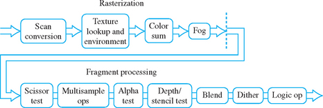
The result of the rasterization step is a set of fragments. A fragment is the part of a primitive contained in (i.e. overlapping) a particular pixel; it includes color, window coordinates, and depth information. After rasterization, the fragments undergo a series of processing steps, called fragment operations. These steps include scissoring, alpha test, depth, and stencil test and blending. At the end of fragment operations, the primitive’s fragments have been used to update the framebuffer. If multisample antialiasing is enabled, more complex fragments containing multiple color, texture coordinate, depth, and stencil values are generated and processed for each pixel location the primitive covers.
6.1 Rasterization
OpenGL specifies a specific set of rules to determine which pixels a given primitive covers. Conceptually, the primitive is overlayed on the window space pixel grid. The pixel coverage rules are detailed and vary per primitive, but all pixel coverage is determined by comparing the primitive’s extent against one or more sample points in each pixel. This point sampling method does not compute a primitive’s coverage area; it only computes whether the primitive does or doesn’t cover each of the pixel’s sample points. This means that a primitive can cover a significant portion of a pixel, yet still not affect its color, if none of the pixel’s sample points are covered.
If multisampling is not being used, there is one sample point for each pixel, it is located at the pixel center; in window coordinates this means a pixel at framebuffer location (m, n) is sampled at (m + ![]() , n +
, n + ![]() ). When multisampling is enabled, the number and location of sample points in each pixel is implementation-dependent. In addition to some number of samples per-pixel, there is a single per-pixel coverage value with as many bits as there are pixel samples. The specification allows the color and texture values to be the same for all samples within a pixel; only the depth and stencil information must represent the values at the sample point. When rasterizing, all sample information for a pixel is bundled together into a single fragment. There is always exactly one fragment per-pixel. When multisampling is disabled, two adjacent primitives sharing a common edge also generate one fragment per-pixel. With multisampling enabled, two fragments (one from each primitive) may be generated at pixels along the shared edge, since each primitive may cover a subset of the sample locations within a pixel.
). When multisampling is enabled, the number and location of sample points in each pixel is implementation-dependent. In addition to some number of samples per-pixel, there is a single per-pixel coverage value with as many bits as there are pixel samples. The specification allows the color and texture values to be the same for all samples within a pixel; only the depth and stencil information must represent the values at the sample point. When rasterizing, all sample information for a pixel is bundled together into a single fragment. There is always exactly one fragment per-pixel. When multisampling is disabled, two adjacent primitives sharing a common edge also generate one fragment per-pixel. With multisampling enabled, two fragments (one from each primitive) may be generated at pixels along the shared edge, since each primitive may cover a subset of the sample locations within a pixel.
Irrespective of the multisample state, each sample holds color, depth, stencil, and texture coordinate information from the primitive at the sample location. If multitexturing is supported, the sample contains texture coordinates for each texture unit supported by the implementation.
Often implementations will use the same color and texture coordinate values for each sample position within a fragment. This provides a significant performance advantage since it reduces the number of distinct sample values that need to be computed and transmitted through the remainder of the fragment processing path. This form of multisample antialiasing is often referred to as edge antialiasing, since the edges of geometric primitives are effectively supersampled but interior colors and texture coordinates are not. When fragments are evaluated at a single sample position, care must be taken in choosing it. In non-multisampled rasterization, the color and texture coordinate values are computed at the pixel center. In the case of multisampling, the color value must be computed at a sample location that is within the primitive or the computed color value may be out of range. However, texture coordinate values are sampled at the pixel center since the wrapping behavior defined for texture coordinates will ensure that an in-range value is computed. Two reasonable choices an implementation may use for the color sample location are the sample nearest the center of the pixel or the sample location closest to the centroid of the sample locations (the average) within the primitive.
6.1.1 Rasterization Consistency
The OpenGL specification does not dictate a specific algorithm for rasterizing a geometric primitive. This lack of precision is deliberate; it allows implementors freedom to choose the best algorithm for their graphics hardware and software. While good for the implementor, this lack of precision imposes restrictions on the design of OpenGL applications. The application cannot make assumptions about exactly how a primitive is rasterized. One practical implication: an application shouldn’t be designed to assume that a primitive whose vertex coordinates don’t exactly match another primitive’s will still have the same depth or color values. This can be restrictive on algorithms that require coplanar polygons.
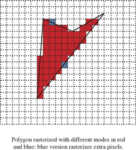
This lack of consistency also affects primitives that have matching vertices, but are rendered with different rasterization modes. The same triangle drawn with GL_FILL and GL_LINE rendering modes may not generate matching depth or color values, or even cover the same pixels along its outer boundary.
OpenGL consistency guidelines do require that certain changes, such as changes in vertex color, texture coordinate position, current texture, and a host of other state changes, will not affect the depth or pixel coverage of a polygon. If these consistency rules were not required, it would be very difficult or impossible to perform many of the techniques described in this book. This is because many of the book’s techniques draw an object multiple times, each time with different parameter settings. These multipass algorithms combine the results of rendering objects multiple times in order to create a desired effect (Figure 6.2).
6.1.2 Z-Fighting
One consequence of inconsistent rendering is depth artifacts. If the depth information of multiple objects (or the same object rendered multiple times) does not match fragment for fragment, the results of depth testing can create artifacts in the color buffer. This problem, commonly known as z-fighting, creates unwanted artifacts that have a “stitched” appearance. They appear where two objects are rasterized into fragments with depth values that differ a very small amount, and were rendered using different algorithms.
Z-fighting can happen when attempting to position and draw two different objects in the same plane. Because of differences in rasterization, the two coplanar objects may not rasterize to the same depth values at all fragments. Figure 6.3 shows two triangles drawn in the same plane. Some of the fragments from the farther triangle have replaced fragments from the closer triangle. At these fragment locations, rasterization of the farther triangle has generated a depth value that is smaller than the one generated by the closer one. The depth test discards the fragments from the closer triangle, since it is configured to keep fragments with smaller depth values. The problem is exacerbated when the scene is animated, since different pixels may bleed through as the primitives change orientation. These problems result from numerical rounding errors; they become significant because the depth values for the fragments are so close together numerically.

There are a number of ways to avoid z-fighting. If two coplanar polygons are required, the application can take care to use the same vertices for both of them, and set their states to ensure that the same rasterization method is used on both of them. If this isn’t possible, the application can choose to disable depth testing altogether, and use the stencil buffer for any masking that is required (Section 16.8). Another approach is to displace one of the two polygons toward the viewer, so the polygons are separated enough in depth that rasterization differences won’t cause one polygon to “bleed through” another. Care should be taken with this last approach, since the choice of polygon that should be displaced toward the viewer may be orientation-dependent. This is particularly true if back-facing polygons are used by the application.
OpenGL does provide a mechanism to make the displacement method more convenient, called polygon offset. Using the glPolygonOffset command allows the programmer to set a displacement for polygons based on their slope and a bias value. The current polygon offset can be enabled separately for points, lines and polygons, and the bias and slope values are signed, so that a primitive can be biased toward or away from the viewer. This relieves the application from the burden of having to apply the appropriate offset to primitive vertices in object space, or adjusting the modelview matrix. Some techniques using polygon offset are described in Section 16.7.2.
6.1.3 Bitmaps and Pixel Rectangles
Points, lines, and polygons are not the only primitives that are rasterized by OpenGL. Bitmaps and pixel rectangles are also available. Since rasterized fragments require window coordinates and texture coordinates as well as color values, OpenGL must generate the x, y, and z values, as well as a set of texture coordinates for each pixel and bitmap fragment. OpenGL uses the notion of a raster position to augment the pixel rectangles and bitmaps with additional position information. A raster position corresponds to the lower left corner of the rectangular pixel object. The glRasterPos command provides the position of the lower left corner of the pixel rectangle; it is similar to the glVertex call in that there are 2-, 3-, and 4-component versions, and because it binds the current texture coordinate set and color to the pixel primitive.
The coordinates of a raster position can be transformed like any vertex, but only the raster position itself is transformed; the pixel rectangle is always perpendicular to the viewer. Its lower left corner is attached to the raster position, and all of its depth values match the raster position’s z coordinate. Similarly, the set texture coordinates and color associated with the raster position are used as the texture coordinates for all the fragments in the pixel primitive.
6.1.4 Texture, Color, and Depth Interpolation
Although it doesn’t define a specific algorithm, the OpenGL specification provides specific guidelines on how texture coordinates, color values, and depth values are calculated for each fragment of a primitive during rasterization. For example, rasterization of a polygon involves choosing a set of fragments corresponding to pixels “owned” by the polygon, interpolating the polygon’s vertex parameters to find their values at each fragment, then sending these fragments down the rest of the pipeline. OpenGL requires that the algorithm used to interpolate the vertex values must behave as if the parameters are calculated using barycentric coordinates. It also stipulates that the x and y values used for the interpolation of each fragment must be computed at the pixel center for that fragment.
Primitive interpolation generates a color, texture coordinates, and a depth value for each fragment as a function of the x and y window coordinates for the fragment (multiple depth values per-pixel may be generated if multisampling is active and multiple texture coordinates may be compared when multitexture is in use). Conceptually, this interpolation is applied to primitives after they have been transformed into window coordinates. This is done so pixel positions can be interpolated relative to the primitive’s vertices. While a simple linear interpolation from vertices to pixel locations produces correct depth values for each pixel, applying the same interpolation method to color values is problematic, and texture coordinates interpolated in this manner can cause visual artifacts. A texture coordinate interpolated in window space may simply not produce the same result as would interpolating to the equivalent location on the primitive in clip space.
These problems occur if the transformation applied to the primitive to go from clip space into window space contains a perspective projection. This is a non-linear transform, so a linear interpolation in one space won’t produce the same results in the other. To get the same results in both spaces, even if a perspective transform separates them, requires using an interpolation method that is perspective invariant.
A perspective-correct method interpolates the ratio of the interpolants and a w term to each pixel location, then divides out the w term to get the interpolated value. Values at each vertex are transformed by dividing them by the w value at the vertex. Assume a clip-space vertex a with associated texture coordinates sa and ta, and a w value of wa. In order to interpolate these values, create new values at the vertex, ![]() , and
, and ![]() . Do this for the values at each vertex in the primitive, then interpolate all the terms (including the
. Do this for the values at each vertex in the primitive, then interpolate all the terms (including the ![]() values) to the desired pixel location. The interpolated texture coordinates ratios are obtained by dividing the interpolated
values) to the desired pixel location. The interpolated texture coordinates ratios are obtained by dividing the interpolated ![]() and
and ![]() values by the interpolated
values by the interpolated ![]() and
and ![]() which results in a perspective-correct s and t.
which results in a perspective-correct s and t.
Here is another example, which shows a simple interpolation using this method in greater detail. A simple linear interpolation of a parameter f, between points a and b uses the standard linear interpolation formula:
Interpolating in a perspective-correct manner changes the formula to:
The OpenGL specification strongly recommends that texture coordinates be calculated in a “perspective correct” fashion, while depth values should not be (depth values will maintain their correct depth ordering even across a perspective transform). Whether to use a perspective correct interpolation of per-fragment color values is left up to the implementation. Recent improvements in graphics hardware make it possible for some OpenGL implementations to efficiently perform the interpolation operations in clip space rather than window space.
Finally, note that the texture coordinates are subjected to their own perspective division by q. This is included, as part of the texture coordinate interpolation, changing Equation 6.1 to:
6.1.5 w Buffering
Although the OpenGL specification specifies the use of the zw fragment component for depth testing, some implementations use a per-fragment w component instead. This may be done to eliminate the overhead of interpolating a depth value; a per-pixel ![]() value must be computed for perspective correct texturing, so per-pixel computation and bandwidth can be reduced by eliminating z and using w instead. The w component also has some advantages when used for depth testing. For a typical perspective transform (such as the one generated by using glFrustum), the transformed w component is linearly related to the pre-transformed z component. On the other hand, the post-transformed z is related to the pre-transformed
value must be computed for perspective correct texturing, so per-pixel computation and bandwidth can be reduced by eliminating z and using w instead. The w component also has some advantages when used for depth testing. For a typical perspective transform (such as the one generated by using glFrustum), the transformed w component is linearly related to the pre-transformed z component. On the other hand, the post-transformed z is related to the pre-transformed ![]() (see Section 2.8 for more details on how z coordinates are modified by a perspective projection).
(see Section 2.8 for more details on how z coordinates are modified by a perspective projection).
Using w instead of z results in a depth buffer with a linear range. This has the advantage that precision is distributed evenly across the range of depth values. However, this isn’t always an advantage since some applications exploit the improved effective resolution present in the near range of traditional depth buffering in w Pleasure, w Fun (1998), Jim Blinn analyzes the characteristics in detail). Furthermore, depth buffer reads on an implementation using w buffering produces very implementation-specific values, returning w values or possibly ![]() values (which are more “z-like”). Care should be taken using an algorithm that depends on retrieving z values when the implementation uses w buffering.
values (which are more “z-like”). Care should be taken using an algorithm that depends on retrieving z values when the implementation uses w buffering.
6.2 Fragment Operations
A number of fragment operations are applied to rasterization fragments before they are allowed to update pixels in the framebuffer. Fragment operations can be separated into two categories, operations that test fragments, and operations that modify them. To maximize efficiency, the fragment operations are ordered so that the fragment tests are applied first. The most interesting tests for advanced rendering are: alpha test, stencil test, and depth buffer test. These tests can either pass, allowing the fragment to continue, or fail, discarding the fragment so it can’t pass on to later fragment operations or update the framebuffer. The stencil test is a special case, since it can produce useful side effects even when fragments fail the comparison.
All of the fragment tests use the same set of comparison operators: Never, Always, Less, Less than or Equal, Equal, Greater than or Equal, Greater, and Not Equal. In each test, a fragment value is compared against a reference value saved in the current OpenGL state (including the depth and stencil buffers), and if the comparison succeeds, the test passes. The details of the fragment tests are listed in Table 6.1.
Table 6.1
| Constant | Comparison |
| GL_ALWAYS | always pass |
| GL_NEVER | never pass |
| GL_LESS | pass if incoming < ref |
| GL_LEQUAL | pass if incoming ≤ ref |
| GL_GEQUAL | pass if incoming ≥ ref |
| GL_GREATER | pass if incoming > ref |
| GL_EQUAL | pass if incoming = ref |
| GL_NOTEQUAL | pass if incoming ≠ ref |
The list of comparison operators is very complete. In fact, it may seem that some of the comparison operations, such as GL_NEVER and GL_ALWAYS are redundant, since their functionality can be duplicated by enabling or disabling a given fragment test. There is a use for them, however. The OpenGL invariance rules require that invariance is maintained if a comparison is changed, but not if a test is enabled or disabled. So if invariance must be maintained (because the test is used in a multipass algorithm, for example), the application should enable and disable tests using the comparison operators, rather than enabling or disabling the tests themselves.
6.2.1 Multisample Operations
Multisample operations provide limited ways to affect the fragment coverage and alpha values. In particular, an application can reduce the coverage of a fragment, or convert the fragment’s alpha value to another coverage value that is combined with the fragment’s value to further reduce it. These operations are sometimes useful as an alternative to alpha blending, since they can be more efficient.
6.2.2 Alpha Test
The alpha test reads the alpha component value of each fragment’s color, and compares it against the current alpha test value. The test value is set by the application, and can range from zero to one. The comparison operators are the standard set listed in Table 6.1. The alpha test can be used to remove parts of a primitive on a pixel by pixel basis. A common technique is to apply a texture containing alpha values to a polygon. The alpha test is used to trim a simple polygon to a complex outline stored in the alpha values of the surface texture. A detailed description of this technique is available in Section 14.5.
6.2.3 Stencil Test
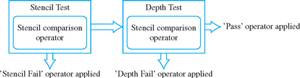
The stencil test performs two tasks. The first task is to conditionally eliminate incoming fragments based on a comparison between a reference value and stencil value from the stencil buffer at the fragment’s destination. The second purpose of the stencil test is to update the stencil values in the framebuffer. How the stencil buffer is modified depends on the outcome of the stencil and depth buffer tests. There are three possible outcomes of the two tests: the stencil buffer test fails, the stencil buffer test passes but the depth buffer fails, or both tests fail. OpenGL makes it possible to specify how the stencil buffer is updated for each of these possible outcomes.
The conditional elimination task is controlled with glStencilFunc. It sets the stencil test comparison operator. The comparison operator can be selected from the list of operators in Table 6.1.
Setting the stencil update requires setting three parameters, each one corresponding to one of the stencil/depth buffer test outcomes. The glStencilOp command takes three operands, one for each of the comparison outcomes (see Figure 6.4). Each operand value specifies how the stencil pixel corresponding to the fragment being tested should be modified. Table 6.2 shows the possible values and how they change the stencil pixels.
Table 6.2
| Constant | Description |
| GL_KEEP | stencil pixel←old value |
| GL_ZERO | stencil pixel←0 |
| GL_REPLACE | stencil pixel←reference value |
| GL_INCR | stencil pixel←old value+1 |
| GL_DECR | stencil pixel←old value−1 |
| GL_INVERT | stencil pixel←old value |
The stencil buffer is often used to create and use per-pixel masks. The desired stencil mask is created by drawing geometry (often textured with an alpha pattern to produce a complex shape). Before rendering this template geometry, the stencil test is configured to update the stencil buffer as the mask is rendered. Often the pipeline is configured so that the color and depth buffers are not actually updated when this geometry is rendered; this can be done with the glColorMask and glDepthMask commands, or by setting the depth test to always fail.
Once the stencil mask is in place, the geometry to be masked is rendered. This time, the stencil test is pre-configured to draw or discard fragments based on the current value of the stencil mask. More elaborate techniques may create the mask using a combination of template geometry and carefully chosen depth and stencil comparisons to create a mask whose shape is influenced by the geometry that was previously rendered. There are are also some extensions for enhancing stencil functionality. One allows separate stencil operations, reference value, compare mask, and write mask to be selected depending on whether the polygon is front- or back-facing.1 A second allows the stencil arithmetic operations to wrap rather than clamp, allowing a stencil value to temporarily go out of range, while still producing the correct answer if the final answer lies within the representable range.2
6.2.4 Blending
One of the most useful fragment modifier operations supported by OpenGL is blending, also called alpha blending. Without blending, a fragment that passes all the filtering and modification steps simply replaces the appropriate color pixel in the framebuffer. If blending is enabled, the incoming fragment, the corresponding target pixel, or an application-defined constant color3 are combined using a linear equation instead. The color components (including alpha) of both the fragment and the pixel are first scaled by a specified blend factor, then either added or subtracted.4 The resulting value is used to update the framebuffer.
There are two fixed sets of blend factors (also called weighting factors) for the blend operation; one set is for the source argument, one for the destination. The entire set is listed in Table 6.3; the second column indicates whether the factor can be used with a source, a destination, or both. These factors take a color from one of the three inputs, the incoming fragment, the framebuffer pixel, or the application-specified color, modify it, and insert it into the blending equation. The source and destination arguments are used by the blend equation, one of GL_FUNC_ADD, GL_FUNC_SUBTRACT, GL_FUNC_REVERSE_SUBTRACT, GL_MIN, or GL_MAX. Table 6.4 lists the operations. Note that the result of the subtract equation depends on the order of the arguments, so both subtract and reverse subtract are provided. In either case, negative results are clamped to zero.
Table 6.3
| Constant | Used In | Action |
| GL_ZERO | src, dst | scale each color element by zero |
| GL_ONE | src, dst | scale each element by one |
| GL_SRC_COLOR | dst | scale color with source color |
| GL_DST_COLOR | src | scale color with destination color |
| GL_ONE_MINUS_SRC_COLOR | dst | scale color with one minus source color |
| GL_ONE_MINUS_DST_COLOR | dst | scale color with one minus destination color |
| GL_SRC_ALPHA | src, dst | scale color with source alpha |
| GL_ONE_MINUS_SRC_ALPHA | src, dst | scale color with source alpha |
| GL_DST_ALPHA | src, dst | scale color with destination alpha |
| GL_ONE_MINUS_DST_ALPHA | src, dst | scale color with one minus destination alpha |
| GL_SRC_ALPHA_SATURATE | src | scale color by minimum of source alpha and destination alpha |
| GL_CONSTANT_COLOR | src, dst | scale color with application-specified color |
| GL_ONE_MINUS_CONSTANT_COLOR | src, dst | scale color with one minus application-specified color |
| GL CONSTANT ALPHA | src, dst | scale color with alpha of application-specified color |
| GL_ONE_MINUS_CONSTANT_ALPHA | src, dst | scale color with one minus alpha of application-specified color |
Table 6.4
| Operand | Result |
| GL_ADD | soruce + destination |
| GL_SUBTRACT | source – destination |
| GL_REVERSE_SUBTRACT | destination – source |
| GL_MIN | min(source, dest) |
| GL_MAX | max(source, dest) |
Some blend factors are used more frequently than others: GL_ONE is commonly used when an unmodified source or destination color is needed in the equation. Using GL_ONE for both factors, for example, simply adds (or subtracts) the source pixel and destination pixel value. The GL_ZERO factor is used to eliminate one of the two colors. The GL_SRC_ALPHA/GL_ONE_MINUS_ALPHA combination is used for a common transparency technique, where the alpha value of the fragment determines the opacity of the fragment. Another transparency technique uses GL_SRC_ALPHA_SATURATE instead; it is particularly useful for wireframe line drawings, since it minimizes line brightening where multiple transparent lines overlap.
6.2.5 Logic Op
As of OpenGL 1.1, a new fragment processing stage, logical operation,5 can be used instead of blending (if both stages are enabled by the application, logic op takes precedence, and blending is implicitly disabled). Logical operations are defined for both index and RGBA colors; only the latter is discussed here. As with blending, logic op takes the incoming fragment and corresponding pixel color, and performs an operation on it. This bitwise operation is chosen from a fixed set by the application using the glLogicOp command. The possible logic operations are shown in Table 6.5 (C-style logical operands are used for clarity).
Table 6.5
| Operand | Result |
| GL_CLEAR | 0 |
| GL_AND | source & destination |
| GL_AND_REVERSE | source & ∼destination |
| GL_COPY | source |
| GL_AND_INVERTED | ∼(source & destination) |
| GL_NOOP | destination |
| GL_XOR | source & destination |
| GL_OR | source | destination |
| GL_NOR | ∼(source | destination) |
| GL_EQUIV | ∼(source |
| GL_INVERT | ∼destination |
| GL_OR_REVERSE | source | ∼destination |
| GL_COPY_INVERTED | ∼source |
| GL_OR_INVERTED | ∼source | destination |
| GL_NAND | ∼(source & destination) |
| GL_SET | 1 (all bits) |
Logic ops are applied separately for each color component. Color component updates can be controlled per channel by using the glColorMask command. The default command is GL_COPY, which is equivalent to disabling logic op. Most commands are self-explanatory, although the GL_EQUIV operation may lead to confusion. It can be thought of as an equivalency test; a bit is set where the source and destination bits match.
6.3 Framebuffer Operations
There are a set of OpenGL operations that are applied to the entire framebuffer at once. The accumulation buffer is used in many OpenGL techniques and is described below.
6.3.1 Accumulation Buffer
The accumulation buffer provides accelerated support for combining multiple rendered images together. It is an off-screen framebuffer whose pixels have very high color resolution. The rendered frame and the accumulation buffer are combined by adding the pixel values together, and updating the accumulation buffer with the results. The accumulation buffer has a scale value that can be used to scale the pixels in the rendered frame before its contents are merged with the contents of the accumulation buffer.
Accumulation operations allow the application to combine frames to generate high-quality images or produce special effects. For example, rendering and combining multiple images modified with a subpixel jitter can be used to generate antialiased images.
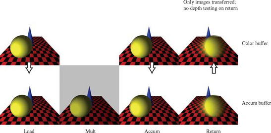
It’s important to understand that the accumulation buffer operations only take input from the color buffer; the OpenGL specification provides no way to render directly to the accumulation buffer. There are a number of consequences to this limitation; it is impossible, for example, to replace part of the image, since there is no depth or stencil buffer available to mask part of the image. The accumulation buffer is best thought of as a place to do high-precision scaling, blending, and clamping of color images. Figure 6.5 shows how multiple images rendered to the color buffer are transferred to the accumulation buffer to be combined together.
Besides having limited access from the rendering pipeline, the accumulation buffer differs from a generic off-screen framebuffer in a number of ways. First, the color representation is different. The accumulation buffer represents color values with component ranges from [−1, 1], not just [0, 1] as in a normal OpenGL framebuffer. As mentioned previously, the color precision of the accumulation buffer is higher than a normal color buffer, often increasing the number of bits representing each color component by a factor of two or more (depending on the implementation). This enhanced resolution increases the number of ways the images can be combined and the number of accumulations that can be performed without degrading image quality.
The accumulation buffer also provides additional ways to combine and modify images. Incoming and accumulation buffer images can be added together, and the accumulation buffer image can be scaled and biased. The return operation, which copies the accumulation buffer back into the framebuffer, also provides implicit image processing functionality: the returned image can be scaled into a range containing negative values, which will be clamped back to the [0, 1] range as it’s returned. Images that are loaded or accumulated into the accumulation buffer can also be scaled as they are copied in. The operations are summarized in Table 6.6.
Table 6.6
Accumulation Buffer Operations
| Constant | Description |
| GL_ACCUM | scale the incoming image, add it to the accumulation buffer |
| GL_LOAD | replace the accumulation buffer with the incoming scaled image |
| GL_ADD | bias the accumulation buffer image |
| GL_MULT | scale the accumulation buffer image |
| GL_RETURN | copy the scaled and clamped accumulation buffer into the color buffer |
Note that the accumulation buffer is often not well accelerated on commodity graphics hardware, so care must be taken when using it in a performance-critical application. There are techniques mentioned later in the book that maximize accumulation buffer performance, and even a slow accumulation buffer implementation can be useful for generating images “off line”. For example, the accumulation buffer can be used to generate high-quality textures and bitmaps to be stored as part of the application, and thus used with no performance penalty.
6.4 Summary
The details of this section of the OpenGL pipeline have a large influence on the design of a multipass algorithm. The rasterization and fragment processing operations provide many mechanisms for modifying a fragment value or discarding it outright.
Over the last several chapters we have covered the rendering pipeline from front to back. In the remainder of this part of the book we will round out our understanding of the pipeline by describing how the rendering pipeline is integrated into the native platform window system, examining some of the evolution of the OpenGL pipeline, and exploring some of the techniques used in implementing hardware and software versions of the pipeline.