Appendix B. Solution of the Stress Cubic Equation

B.1 Principal Stresses

There are many methods in common usage for solving a cubic equation. A simple approach for dealing with Eq. (1.33) is to find one root, say σ₁, by plotting it (σ as abscissa) or by trial and error. The cubic equation is then factored by dividing by (σ_p – σ₁) to arrive at a quadratic equation. The remaining roots can be obtained by applying the familiar general solution of a quadratic equation. This process requires considerable time and algebraic work, however.

What follows is a practical approach for determining the roots-of-stress cubic equation (1.33):

(a)

where

(B.1)

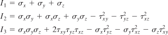
According to the method, expressions that provide direct means for solving both two- and three-dimensional stress problems are [Refs. B.1 and B.2]

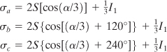
(B.2)

Here the constants are given by

(B.3)

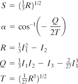
and invariants I₁, I₂, and I₃ are represented in terms of the given stress components by Eqs. (B.1).

The principal stresses found from Eqs. (B.2) are redesignated using numerical subscripts so that σ₁ > σ₂ > σ₃. This procedure is well adapted to a pocket calculator or digital computer.

B.2 Direction Cosines

The values of the direction cosines of a principal stress are determined through the use of Eqs. (1.31) and (1.25), as discussed in Section 1.13. That is, substitution of a principal stress, say σ₁, into Eqs. (1.31) results in two independent equations in three unknown direction cosines. From these expressions, together with , we obtain l₁, m₁, and n₁.

However, instead of solving one second-order and two linear equations simultaneously, the following simpler approach is preferred. Expressions (1.31) are expressed in matrix form as follows:

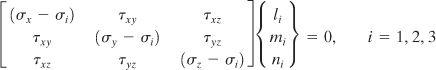
The cofactors of the determinant of this matrix on the elements of the first row are

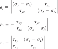
(B.4)

Upon introduction of the notation

(B.5)

the direction cosines are then expressed as

(B.6)

It is clear that Eqs. (B.6) lead to .

Application of Eqs. (B.2) and (B.6) to the sample problem described in Example 1.6 provides some algebraic exercise. Substitution of the given data into Eqs. (B.1) results in

We then have

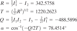
Hence, Eqs. (B.2) give

Reordering and redesignating these values,

from which it follows that

and

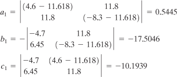
Thus, Eqs. (B.6) yield

As a check, . Repeating the same procedure for σ₂ and σ₃, we obtain the values of direction cosines given in Example 1.6.

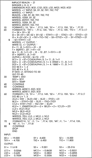
A FORTRAN computer program is listed in Table B.1 to expedite the solution for the principal stresses and associated direction cosines. Input data and output values are also provided. The program was written and tested on a digital computer. Note that this listing may readily be extended to obtain the factors of safety according to the various theories of failure (Chap. 4).

Table B.1. FORTRAN Program for Principal Stresses

References

B.1. MESSAL, E. E., Finding true maximum shear stress, Mach. Des., December 7, 1978, pp. 166–169.

B.2. TERRY, E. S., A Practical Guide to Computer Methods for Engineers, Prentice Hall, Englewood Cliffs, N. J., 1979.