Chapter 2. Strain and Material Properties
2.1 Introduction
In Chapter 1, our concern was with the stresses within a body subject to a system of external forces. We now turn to the deformations caused by these forces and to a measure of deformational intensity called strain, discussed in Sections 2.3 through 2.5. Deformations and strains, which are necessary to an analysis of stress, are also important quantities in themselves, for they relate to changes in the size and shape of a body.
Recall that the state of stress at a point can be determined if the stress components on mutually perpendicular planes are given. A similar operation applies to the state of strain to develop the transformation relations that give two-dimensional and three-dimensional strains in inclined directions in terms of the strains in the coordinate directions. The plane strain transformation equations are especially important in experimental investigations, where normal strains are measured with strain gages. It is usually necessary to use some combination of strain gages or a strain rosette, with each gage measuring the strain in a different direction.
The mechanical properties of engineering materials, as determined from tension test, are considered in Sections 2.6 through 2.8. Material selection and stress–strain curves in tension, compression, and shear are also briefly discussed. Following this, there is a discussion of the relationship between strain and stress under uniaxial, shear, and multiaxial loading conditions. The measurement of strain and the concept of strain energy are taken up in Sections 2.12 through 2.15. Finally, Saint-Venant’s principle, which is extremely useful in the solution of practical problems, is introduced in Section 2.16.
2.2 Deformation
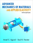
Let us consider a body subjected to external loading that causes it to take up the position pictured by the dashed lines in Fig. 2.1, in which A is displaced to A′, B to B′, and so on, until all the points in the body are displaced to new positions. The displacements of any two points such as A and B are simply AA′ and BB′, respectively, and may be a consequence of deformation (straining), rigid-body motion (translation and rotation), or some combination. The body is said to be strained if the relative positions of points in the body are altered. If no straining has taken place, displacements AA′ and BB′ are attributable to rigid-body motion. In the latter case, the distance between A and B remains fixed; that is, L0 = L. Such displacements are not discussed in this chapter.
Figure 2.1. Plane displacement and strain in a body.

To describe the magnitude and direction of the displacements, points within the body are located with respect to an appropriate coordinate reference as, for example, the xyz system. Therefore, in the two-dimensional case shown in Fig. 2.1, the components of displacement of point A to A′ can be represented by u and v in the x and y coordinate directions, respectively. In general, the components of displacement at a point, occurring in the x, y, and z directions, are denoted by u, v, and w, respectively. The displacement at every point within the body constitutes the displacement field, u = u(x, y, z), v = v(x, y, z), and w = w(x, y, z). In this text, mainly small displacements are considered, a simplification consistent with the magnitude of deformation commonly found in engineering structures. The strains produced by small deformations are small compared to unity, and their products (higher-order terms) are neglected. For purposes of clarity, small displacements with which we are concerned will be shown highly exaggerated on all diagrams.
Superposition
The small displacement assumption leads to one of the basic fundamentals of solid mechanics, called the principle of superposition. This principle is valid whenever the quantity (stress or displacement) to be determined is a linear function of the loads that produce it. For the foregoing condition to exist, material must be linearly elastic. In such situations, the total quantity owing to the combined loads acting simultaneously on a member may be obtained by determining separately the quantity attributable to each load and combining the individual results.
For example, normal stresses caused by axial forces and bending simultaneously (see Table 1.1) may be obtained by superposition, provided that the combined stresses do not exceed the proportional limit of the material. Likewise, shearing stresses caused by a torque and a vertical shear force acting simultaneously in a beam may be treated by superposition. Clearly, superposition cannot be applied to plastic deformations. The principle of superposition is employed repeatedly in this text. The motivation for superposition is the replacement of a complex load configuration by two or more simpler loads.
2.3 Strain Defined
For purposes of defining normal strain, refer to Fig. 2.2, where line AB of an axially loaded member has suffered deformation to become A′B′. The length of AB is Δx (Fig. 2.2a). As shown in Fig. 2.2b, points A and B have each been displaced: A an amount u, and B, u + Δu. Stated differently, point B has been displaced by an amount Δu in addition to displacement of point A, and the length Δx has been increased by Δu. Normal strain, the unit change in length, is defined as
(2.1)
Figure 2.2. Normal strain in a prismatic bar: (a) undeformed state; (b) deformed state.

In view of the limiting process, Eq. (2.1) represents the strain at a point, the point to which Δx shrinks.
If the deformation is distributed uniformly over the original length, the normal strain may be written
(2.2)
where L, Lo and δ are the final length, the original length, and the change of length of the member, respectively. When uniform deformation does not occur, the aforementioned is the average strain.
Plane Strain
We now investigate the case of two-dimensional or plane strain, wherein all points in the body, before and after application of load, remain in the same plane. Two-dimensional views of an element with edges of unit lengths subjected to plane strain are shown in three parts in Fig. 2.3. We note that this element has no normal strain εz and no shearing strains γxz and γyz in the xz and yz planes, respectively.
Figure 2.3. Strain components εx, εy, and γxy in the xy plane.

Referring to Fig. 2.4, consider an element with dimensions dx, dy and of unit thickness. The total deformation may be regarded as possessing the following features: a change in length experienced by the sides (Fig. 2.4a) and a relative rotation without accompanying changes of length (Fig. 2.4b).
Figure 2.4. Deformations of an element: (a) normal strain; (b) shearing strain.
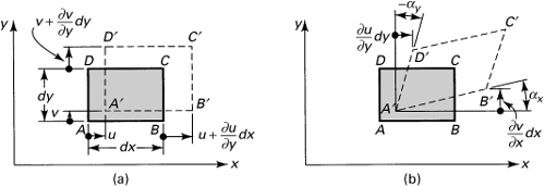
Recalling the basis of Eq. (2.1), two normal or longitudinal strains are apparent upon examination of Fig. 2.4a:
(2.3a)
A positive sign is applied to elongation; a negative sign, to contraction.
Now consider the change experienced by right angle DAB (Fig. 2.4b). We shall assume the angle αx between AB and A′B′ to be so small as to permit the approximation αx ≈ tan αx. Also, in view of the smallness of αx, the normal strain is small, so AB ≈ A′B′. As a consequence of the aforementioned considerations, αx ≈ ∂v/∂x, where the counterclockwise rotation is defined as positive. Similar analysis leads to –αy ≈ ∂u/∂y. The total angular change of angle DAB, the angular change between lines in the x and y directions, is defined as the shearing strain and denoted by γxy:
(2.3b)
The shear strain is positive when the right angle between two positive (or negative) axes decreases. That is, if the angle between +x and +y or –x and –y decreases, we have positive γxy; otherwise the shear strain is negative.
Three-Dimensional Strain
In the case of a three-dimensional element, a rectangular prism with sides dx, dy, dz, an essentially identical analysis leads to the following normal and shearing strains:

(2.4)
Clearly, the angular change is not different if it is said to occur between the x and y directions or between the y and x directions; γxy = γyx. The remaining components of shearing strain are similarly related:
![]()
The symmetry of shearing strains may also be deduced from an examination of Eq. (2.4). The expressions (2.4) are the strain–displacement relations of continuum mechanics. They are also referred to as the kinematic relations, treating the geometry of strain rather than the matter of cause and effect.
A succinct statement of Eq. (2.3) is made possible by tensor notation:
(2.5a)
or expressed more concisely by using commas,
(2.5b)
where ux = u, uy = v, xx = x, and so on. The factor ![]() in Eq. (2.5) facilitates the representation of the strain transformation equations in indicial notation. The longitudinal strains are obtained when i = j; the shearing strains are found when i ≠ j and εij = εji. It is apparent from Eqs. (2.4) and (2.5) that
in Eq. (2.5) facilitates the representation of the strain transformation equations in indicial notation. The longitudinal strains are obtained when i = j; the shearing strains are found when i ≠ j and εij = εji. It is apparent from Eqs. (2.4) and (2.5) that
(2.6)
Just as the state of stress at a point is described by a nine-term array, so Eq. (2.5) represents nine strains composing the symmetric strain tensor (εij = εji):

(2.7)
It is interesting to observe that the Cartesian coordinate systems of Chapters 1 and 2 are not identical. In Chapter 1, the equations of statics pertain to the deformed state, and the coordinate set is thus established in a deformed body; xyz is, in this instance, a Eulerian coordinate system. In discussing the kinematics of deformation in this chapter, recall that the xyz set is established in the undeformed body. In this case, xyz is referred to as a Lagrangian coordinate system. Although these systems are clearly not the same, the assumption of small deformation permits us to regard x, y, and z, the coordinates in the undeformed body, as applicable to equations of stress or strain. Choice of the Lagrangian system should lead to no errors of consequence unless applications in finite elasticity or large deformation theory are attempted. Under such circumstances, the approximation discussed is not valid, and the resulting equations are more difficult to formulate [Refs. 2.1 and 2.2].
Throughout the text, strains are indicated as dimensionless quantities. The normal and shearing strains are also frequently described in terms of units such as inches per inch or micrometers per meter and radians or microradians, respectively. The strains for engineering materials in ordinary use seldom exceed 0.002, which is equivalent to 2000 × 10–6 or 2000 μ. We read this as “2000 micros.”
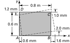
Example 2.1. Plane Strains in a Plate
A 0.8-m by 0.6-m rectangle ABCD is drawn on a thin plate prior to loading. Subsequent to loading, the deformed geometry is shown by the dashed lines in Fig. 2.5. Determine the components of plane strain at point A.
Figure 2.5. Example 2.1. Deformation of a thin plate.
Solution
The following approximate version of the strain–displacement relations of Eqs. (2.3) must be used:
(2.8)
Thus, by setting Δx = 800 mm and Δy = 600 mm, the normal strains are calculated as follows:

In a like manner, we obtain the shearing strain:
![]()
The positive sign indicates that angle BAD has decreased.
Large Strains
As pointed out in Section 2.1, the small deformations or deflections are considered in most applications of this book. The preceding is consistent with the magnitude of deformations usually found in engineering practice. The following more general large or finite strain–displacement relationships are included here so that the reader may better understand the approximations resulting in the relations of small-deformation theory.
When displacements are relatively large, the strain components are given in terms of the square of the element length instead of the length itself. Therefore, with reference to Fig. 2.4b, we write
(2.9)
in which

and AD = dx.
Carrying the foregoing terms into Eq. (2.9) leads to a two-dimensional finite normal strain–displacement relationship:
(2.10a)
Likewise, we have
(2.10b)
It can also be verified [Refs. 2.3 and 2.4], that the finite shearing strain–displacement relation is
(2.10c)
In small displacement theory, the higher-order terms in Eqs. (2.10) are omitted. In so doing, these equations reduce to Eqs. (2.4), as expected. The expressions for three-dimensional state of strain may readily be generalized from the preceding equations.
2.4 Equations of Compatibility
The concept of compatibility has both mathematical and physical significance. From a mathematical point of view, it asserts that the displacements u, v, and w match the geometrical boundary conditions and are single-valued and continuous functions of position with which the strain components are associated [Refs. 2.1 and 2.2]. Physically, this means that the body must be pieced together; no voids are created in the deformed body.
Recall, for instance, the uniform state of stress at a section a–a of an axially loaded member as shown in Fig. 1.5b (Sec. 1.6). This, as well as any other stress distribution symmetric with respect to the centroidal axis, such as a parabolic distribution, can ensure equilibrium provided that ∫ σx dA = P. However, the reason the uniform distribution is the acceptable or correct one is that it also ensures a piece-wise-continuous strain and displacement field consistent with the boundary conditions of the axially loaded member, the essential characteristic of compatibility.
We now develop the equations of compatibility, which establish the geometrically possible form of variation of strains from point to point within a body. The kinematic relations, Eqs. (2.4), connect six components of strain to only three components of displacement. We cannot therefore arbitrarily specify all the strains as functions of x, y, and z. As the strains are evidently not independent of one another, in what way are they related? In two-dimensional strain, differentiation of εx twice with respect to y, εy twice with respect to x, and γxy with respect to x and y results in

or
(2.11)
This is the condition of compatibility of the two-dimensional problem, expressed in terms of strain. The three-dimensional equations of compatibility are obtained in a like manner:

(2.12)
These equations were first derived by Saint-Venant in 1860. The application of the equations of compatibility is illustrated in Example 2.2(a) and in various sections that use the method of the theory of elasticity.
To gain further insight into the meaning of compatibility, imagine an elastic body subdivided into a number of small cubic elements prior to deformation. These cubes may, upon loading, be deformed into a system of parallelepipeds. The deformed system will, in general, be impossible to arrange in such a way as to compose a continuous body unless the components of strain satisfy the equations of compatibility.
2.5 State of Strain at a Point
Recall from Chapter 1 that, given the components of stress at a point, it is possible to determine the stresses on any plane passing through the point. A similar operation pertains to the strains at a point.
Consider a small linear element AB of length ds is an unstrained body (Fig. 2.6a). The projections of the element on the coordinate axes are dx and dy. After straining, AB is displaced to position A′B′ and is now ds′ long. The x and y displacements are u + du and v + dv, respectively. The variation with position of the displacement is expressed by a truncated Taylor’s expansion as follows:
(a)
Figure 2.6. Plane straining of an element.

Figure 2.6b shows the relative displacement of B with respect to A, the straining of AB. It is observed that AB has been translated so that A coincides with A′; it is now in the position A′B″. Here B″ D = du and DB′ = dv are the components of displacement.
Transformation of Two-Dimensional Strain
We now choose a new coordinate system x′ y′, as shown in Fig. 2.6, and examine the components of strain with respect to it: εx′, εy′, γx′y′. First we determine the unit elongation of ds′, εx′. The projections of du and dv on the x′ axis, after taking EB′ cos α = EB′(1) by virtue of the small angle approximation, lead to the approximation (Fig. 2.6b)
(b)
By definition, εx′ is found from EB′/ds. Thus, applying Eq. (b) together with Eqs. (a), we obtain
![]()
Substituting cos θ for dx/ds, sin θ for dy/ds, and Eq. (2.3) into this equation, we have
(2.13a)
This represents the transformation equation for the x-directed normal strain, which, through the use of trigonometric identities, may be converted to the form
(2.14a)
The normal strain εy′ is determined by replacing θ by θ + π/2 in Eq. (2.14a).
To derive an expression for the shearing strain γx′y′, we first determine the angle α through which AB (the x′ axis) is rotated. Referring again to Fig. 2.6b, tan α = B″ E/ds, where B″E = dv cos θ – du sin θ – EB′ sin α. By letting sin α = tan α = α, we have EB′ sin α = εx′ ds α = 0. The latter is a consequence of the smallness of both εx′ and α. Substituting Eqs. (a) and (2.3) into B″E, α = B″ E/ds may be written as follows:
(c)
Next, the angular displacement of y′ is readily derived by replacing θ by θ + π/2 in Eq. (c):
![]()
Now, taking counterclockwise rotations to be positive (see Fig. 2.4b), it is necessary, in finding the shear strain γx′y′, to add α and –αθ + π/2. By so doing and substituting γxy = ∂v/∂x + ∂u/∂y, we obtain
(2.13b)
Through the use of trigonometric identities, this expression for the transformation of the shear strain becomes
(2.14b)
Comparison of Eqs. (1.18) with Eqs. (2.14), the two-dimensional transformation equations of strain, reveals an identity of form. It is observed that transformations expressions for stress are converted into strain relationships by replacing
![]()
These substitutions can be made in all the analogous relations. For instance, the principal strain directions (where γx′y′ = 0) are found from Eq. (1.19):
(2.15)
Similarly, the magnitudes of the principal strains are
(2.16)
The maximum shearing strains are found on planes 45° relative to the principal planes and are given by
(2.17)
Transformation of Three-Dimensional Strain
This case may also proceed from the corresponding stress relations by replacing σ by ε and τ by γ/2. Therefore, using Eqs. (1.28), we have
(2.18a)
(2.18b)
(2.18c)
(2.18d)
(2.18e)
(2.18f)
where l1 is the cosine of the angle between x and x′, m1 is the cosine of the angle between y and x′, and so on (see Table 1.2). The foregoing equations are succinctly expressed, referring to Eqs. (1.29), as follow:
(2.19a)
Conversely,
(2.19b)
These equations represent the law of transformation for a strain tensor of rank 2.
Also, referring to Eqs. (1.33) and (1.34), the principal strains in three dimensions are the roots of the following cubic equation:
(2.20)
The strain invariants are

(2.21)
For a given state of strain, the three roots ε1, ε2, and ε3 of Eqs. (2.20) and the corresponding direction cosines may conveniently be computed using Table B.1 with some notation modification.
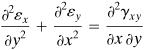
Example 2.2. Three-Dimensional Strain in a Block
A 2-m by 1.5-m by 1-m parallelepiped is deformed by movement of corner point A to A′ (1.9985, 1.4988, 1.0009), as shown by the dashed lines in Fig. 2.7. Calculate the following quantities at point A: (a) the strain components; (b) the normal strain in the direction of line AB; and (c) the shearing strain for perpendicular lines AB and AC.
Figure 2.7. Example 2.2. Deformation of a parallelpiped.

Solution
The components of displacement of point A are given by
(d)
a. We can readily obtain the strain components, by using an approximate version of Eqs. (2.4) and Eqs. (d), as in Example 2.1. Alternatively, these strains can be determined as follows. First, referring to Fig. 2.7, we represent the displacement field in the form
(2.22)
where c1, c2, and c3 are constants. From these and Eqs. (d), –1.5(10–3) = c1(2 × 1.5 × 1) or c1 = –500(10–6); similarly, c2 = –400(10–6), and c3 = 300(10–6). Therefore,
(e)
Applying Eqs. (2.4) and substituting 10–6 = μ, we have
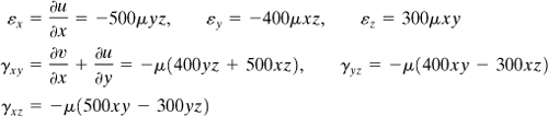
(f)
By introducing the foregoing into Eqs. (2.12), we readily find that these conditions are satisfied and the strain field obtained is therefore possible. The calculations proceed as follows:

b. Let the x′ axis be placed along the line from A to B. The direction cosines of AB are l1 = –0.8, m1 = –0.6, and n1 = 0. Applying Eq. (2.18a), we thus have
![]()
c. Let the y′ axis be placed along the line A to C. The direction cosines of AC are l2 = 0, m2 = 0, and n2 = –1. Thus, from Eq. (2.18b),
![]()
where the negative sign indicates that angle BAC has increased.
Mohr’s Circle for Plane Strain
Because we have concluded that the transformation properties of stress and strain are identical, it is apparent that a Mohr’s circle for strain may be drawn and that the construction technique does not differ from that of Mohr’s circle for stress. In Mohr’s circle for strain, the normal strains are plotted on the horizontal axis, positive to the right. When the shear strain is positive, the point representing the x axis strains is plotted a distance γ/2 below the ε line, and the y axis point a distance γ/2 above the ε line, and vice versa when the shear strain is negative. Note that this convention for shear strain, used only in constructing and reading values from Mohr’s circle, agrees with the convention employed for stress in Section 1.11.
An illustration of the use of Mohr’s circle of strain is given in the solution of the following numerical problem.
Example 2.3. State of Plane Strain in a Plate
The state of strain at a point on a thin plate is given by εx = 510 μ, εy = 120 μ, and γxy = 260 μ. Determine, using Mohr’s circle of strain, (a) the state of strain associated with axes x′, y′, which make an angle θ = 30° with the axes x, y (Fig. 2.8a); (b) the principal strains and directions of the principal axes; (c) the maximum shear strains and associated normal strains; display the given data and the results obtained on properly oriented elements of unit dimensions.
Figure 2.8. Example 2.3: (a) Axes rotated for θ = 30°; (b) Mohr’s circle of strain.

Solution
A sketch of Mohr’s circle of strain is shown in Fig. 2.8b, constructed by determining the position of point C at ![]() and A at
and A at ![]() from the origin O. Note that γxy/2 is positive, so point A, representing x-axis strains, is plotted below the ε axis (or B above). Carrying out calculations similar to that for Mohr’s circle of stress (Sec. 1.11), the required quantities are determined. The radius of the circle is r = (1952 + 1302)1/2 μ = 234 μ, and the angle
from the origin O. Note that γxy/2 is positive, so point A, representing x-axis strains, is plotted below the ε axis (or B above). Carrying out calculations similar to that for Mohr’s circle of stress (Sec. 1.11), the required quantities are determined. The radius of the circle is r = (1952 + 1302)1/2 μ = 234 μ, and the angle ![]() .
.
a. At a position 60° counterclockwise from the x axis lies the x′ axis on Mohr’s circle, corresponding to twice the angle on the plate. The angle A′CA1 is 60° – 33.7° = 26.3°. The strain components associated with x′y′ are therefore

(g)
The shear strain is taken as negative because the point representing the x axis strains, A′, is above the ε axis. The negative sign indicates that the angle between the element faces x′ and y′ at the origin increases (Sec. 2.3). As a check, Eq. (2.14b) is applied with the given data to obtain –207 μ as before.
b. The principal strains, represented by points A1 and B1 on the circle, are found to be
![]()
The axes of ε1 and ε2 are directed at 16.85° and 106.85° from the x axis, respectively.
c. Points D and E represent the maximum shear strains. Thus,
γmax = ±468 μ
Observe from the circle that the axes of maximum shear strain make an angle of 45° with respect to the principal axes. The normal strains associated with the axes of γmax are equal, represented by OC on the circle: 315 μ.
d. The given data is depicted in Fig. 2.9a. The strain components obtained, Eqs. (g), are portrayed in Fig. 2.9b for an element at θ = 30°. Observe that the angle at the corner Q of the element at the origin increases because γxy is negative. The principal strains are given in Fig. 2.9c. The sketch of the maximum shearing strain element is shown in Fig. 2.9d.
Figure 2.9. Example 2.3. (a) Element with edges of unit lengths in plane strain; (b) element at θ = 30°; (c) principal strains; and (d) maximum shearing strains.

2.6 Engineering Materials
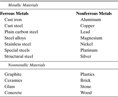
The equations of equilibrium derived in Chapter 1 and the kinematic relations of this chapter together represent nine equations involving 15 unknowns (six stresses, six strains, and three displacements). The insufficiency noted in the number of available equations is made up for by a set of material-dependent relationships, discussed in Section 2.9, that connect stress with strain. We first define some important characteristics of engineering materials, such as those in widespread commercial usage, including a variety of metals, plastics, and concretes. Table 2.1 gives a general classification of materials commonly used in engineering [Refs. 2.5 through 2.8]. Following this, the tension test is discussed (Sec. 2.7), providing information basic to material behavior.
Table 2.1. Typical Engineering Materials
An elastic material is one that returns to its original (unloaded) shape upon the removal of applied forces. Elastic behavior thus precludes permanent or plastic deformation. In many cases, the elastic range includes a region throughout which stress and strain bear a linear relationship. This portion of the stress–strain variation ends at a point termed the proportional limit. Such materials are linearly elastic. It is not necessary for a material to possess such linearity for it to be elastic. In a viscoelastic material, the state of stress is a function not only of the strains but of the time rates of change of stress and strain as well.
Combinations of elastic (springlike) and viscous (dashpotlike) elements form a viscous–elastic model. Glasses, ceramics, biomaterials, synthetic rubbers, and plastics may frequently be considered to be linear viscoelastic materials. Also, most rocks exhibit properties that can be represented by inclusion of viscous terms in the stress–strain relationship. Viscoelastic solids return to their original state when unloaded. A plastically deformed solid, on the other hand, does not return to its original shape when the load is removed; there is some permanent deformation. With the exception of Chapter 12, our considerations will be limited to the behavior of elastic materials.
Leaving out Section 5.9, it is also assumed in this text that the material is homogeneous and isotropic. A homogeneous material displays identical properties throughout. If the properties are identical in all directions at a point, the material is termed isotropic. A nonisotropic or anisotropic solid such as wood displays direction-dependent properties. An orthotropic material, such as wood, is a special case of an anisotropic material, which has greater strength in a direction parallel to the grain than perpendicular to the grain (see Sec. 2.11). Single crystals also display pronounced anisotropy, manifesting different properties along the various crystallographic directions.
Materials composed of many crystals (polycrystalline aggregates) may exhibit either isotropy or anisotropy. Isotropy results when the crystal size is small relative to the size of the sample, provided that nothing has acted to disturb the random distribution of crystal orientations within the aggregate. Mechanical processing operations such as cold rolling may contribute to minor anisotropy, which in practice is often disregarded. These processes may also result in high internal stress, termed residual stress. In the cases treated in this volume, materials are assumed initially entirely free of such stress.
General Properties of Some Common Materials
There are various engineering materials, as listed in Table 2.1. The following is a brief description of a few frequently employed materials. The common classes of materials of engineering interest are metals, plastics, ceramics, and composites. Each group generally has similar properties (such as chemical makeup and atomic structure) and applications. Selection of materials plays a significant role in mechanical design. The choice of a particular material for the members depends on the purpose and type of operation as well as on mode of failure of this component. Strength and stiffness are principal factors considered in selection of a material. But selecting a material from both its functional and economical standpoints is very important. Material properties are determined by standardized test methods outlined by the American Society for Testing Materials (ASTM).
Metals
Metals can be made stronger by alloying and by various mechanical and heat treatments. Most metals are ductile and good conductors of electricity and heat. Cast iron and steel are iron alloys containing over 2% carbon and less than 2% carbon, respectively. Cast irons constitute a whole family of materials including carbon. Steels can be grouped as plain carbon steels, alloy steels, high-strength steels, cast steels, and special-purpose steels. Low-carbon steels or mild steels are also known as the structural steels. There are many effects of adding any alloy to a basic carbon steel. Stainless steels (in addition to carbon) contain at least 12% chromium as the basic alloying element. Aluminum and magnesium alloys possess a high strength-to-weight ratio.
Plastics
Plastics are synthetic materials, also known as polymers. They are used increasingly for structural purposes, and many different types are available. Polymers are corrosion resistant and have low coefficient of friction. The mechanical characteristics of these materials vary notably, with some plastics being brittle and others ductile. The polymers are of two classes: thermoplastics and thermosets. Thermoplastics include acetal, acrylic, nylon, teflon, polypropylene, polystyrene, PVC, and saran. Examples of thermosets are epoxy, polyster, polyurethane, and bakelite. Thermoplastic materials repeatedly soften when heated and harden when cooled. There are also highly elastic flexible materials known as thermoplastic elastomers. A common elastomer is a rubber band. Thermosets sustain structural change during processing; they can be shaped only by cutting or machining.
Ceramics
Ceramics represent ordinary compounds of nonmetallic as well as metallic elements, mostly oxides, nitrides, and carbides. They are considered an important class of engineering materials for use in machine and structural parts. Ceramics have high hardness and brittleness, high compressive but low tensile strengths. High temperature and chemical resistance, high dielectric strength, and low weight characterize many of these materials. Glasses are also made of metallic and nonmetallic elements, just as are ceramics. But glasses and ceramics have different structural forms. Glass ceramics are widely used as electrical, electronic, and laboratory ware.
Composites
Composites are made up of two or more distinct constituents. They often consist of a high-strength material (for example, fiber made of steel, glass, graphite, or polymers) embedded in a surrounding material (such as resin or concrete), which is termed a matrix. Therefore, a composite material shows a relatively large strength-to-weight ratio compared with a homogeneous material; composite materials generally have other desirable characteristics and are widely used in various structures, pressure vessels, and machine components. A composite is designed to display a combination of the best characteristics of each component material. A fiber-reinforced composite is formed by imbedding fibers of a strong, stiff material into a weaker reinforcing material. A layer or lamina of a composite material consists of a variety of arbitrarily oriented bonded layers or laminas. If all fibers in all layers are given the same orientation, the laminate is orthotropic. A typical composite usually consists of bonded three-layer orthotropic material. Our discussions will include isotropic composites like reinforced-concrete beam and multilayered members, single-layer orthotropic materials, and compound cylinders.
2.7 Stress–Strain Diagrams
Let us now discuss briefly the nature of the typical static tensile test. In such a test, a specimen is inserted into the jaws of a machine that permits tensile straining at a relatively low rate (since material strength is strain-rate dependent). Normally, the stress–strain curve resulting from a tensile test is predicated on engineering (conventional) stress as the ordinate and engineering (conventional) strain as the abscissa. The latter is defined by Eq. (2.2). The former is the load or tensile force (P) divided by the original cross-sectional area (Ao) of the specimen and, as such, is simply a measure of load (force divided by a constant) rather than true stress. True stress is the load divided by the actual instantaneous or current area (A) of the specimen.
Ductile Materials in Tension
Figure 2.10a shows two stress–strain plots, one (indicated by a solid line) based on engineering stress, the other on true stress. The material tested is a relatively ductile, polycrystalline metal such as steel. A ductile metal is capable of substantial elongation prior to failure, as in a drawing process. The converse applies to brittle materials. Note that beyond the point labeled “proportional limit” is a point labeled “yield point” (for most cases these two points are taken as one). At the yield point, a great deal of deformation occurs while the applied loading remains essentially constant. The engineering stress curve for the material when strained beyond the yield point shows a characteristic maximum termed the ultimate tensile stress and a lower value, the rupture stress, at which failure occurs. Bearing in mind the definition of engineering stress, this decrease is indicative of a decreased load-carrying capacity of the specimen with continued straining beyond the ultimate tensile stress.
Figure 2.10. (a) Stress–strain diagram of a typical ductile material; (b) determination of yield strength by the offset method.

For materials such as heat-treated steel, aluminum, and copper that do not exhibit a distinctive yield point, it is usual to employ a quasi-yield point. According to the 0.2-percent offset method, a line is drawn through a strain of 0.002, parallel to the initial straight line portion of the curve (Fig. 2.10b). The intersection of this line with the stress–strain curve defines the yield point as shown. Corresponding yield stress is commonly referred to as the yield strength.
Geometry Change of Specimen
In the vicinity of the ultimate stress, the reduction of the cross-sectional area becomes clearly visible, and a necking of the specimen occurs in the range between ultimate and rupture stresses. Figure 2.11 shows the geometric change in the portion of a ductile specimen under tensile loading. The local elongation is always greater in the necking zone than elsewhere. The standard measures of ductility of a material are expressed as follows:
Figure 2.11. A typical round specimen of ductile material in tension: (a) necking; (b) fractured.

(2.23b)
Here Ao and Lo designate, respectively, the initial cross-sectional area and gage length between two punch marks of the specimen. The ruptured bar must be pieced together in order to measure the final gage length Lf. Similarly, the final area Af is measured at the fracture site where the cross section is minimum. The elongation is not uniform over the length of the specimen but concentrated on the region of necking. Percentage of elongation thus depends on the gage length. For structural steel, about 25 percent elongation (for a 50-mm gage length) and 50 percent reduction in area usually occur.
True Stress and True Strain
The large disparity between the engineering stress and true stress curves in the region of a large strain is attributable to the significant localized decrease in area (necking down) prior to fracture. In the area of large strain, particularly that occurring in the plastic range, the engineering strain, based on small deformation, is clearly inadequate. It is thus convenient to introduce true or logarithmic strain. The true strain, denoted by ε, is defined by
(2.24)
This strain is observed to represent the sum of the increments of deformation divided by the length L corresponding to a particular increment of length dL. Here Lo is the original length and εo is the engineering strain.
For small strains, Eqs. (2.2) and (2.24) yield approximately the same results. Note that the curve of true stress versus true strain is more informative in examining plastic behavior and will be discussed in detail in Chapter 12. In the plastic range, the material is assumed to be incompressible and the volume constant (Sec. 2.10). Hence,
(a)
where the left and right sides of this equation represent the original and the current volume, respectively. If P is the current load, then
But, from Eq. (2.2), we have L/Lo = 1 + εo. The true stress is thus defined by
(2.25)
That is, the true stress is equal to the engineering stress multiplied by 1 plus the engineering strain.
A comparison of a true and nominal stress–strain plot is given in Fig. 2.12 [Ref. 2.8]. The true σ – ε curve shows that as straining progresses, more and more stress develops. On the contrary, in the nominal σ – ε curve, beyond the ultimate strength the stress decreases with the increase in strain. This is particularly important for large deformations involved in metal-forming operations [Ref. 2.7].
Figure 2.12. Stress–strain curves for a low-carbon (0.05%) steel in tension.

Brittle Materials in Tension
Brittle materials are characterized by the fact that rupture occurs with little deformation. The behavior of typical brittle materials, such as magnesium alloy and cast iron, under axial tensile loading is shown in Figs. 2.13a. Observe from the diagrams that there is no well-defined linear region, rupture takes place with no noticeable prior change in the rate of elongation, there is no difference between the ultimate stress and the fracture stress, and the strain at rupture is much smaller than in ductile materials. The fracture of a brittle material is associated with the tensile stress. A brittle material thus breaks normal to the axis of the specimen, as depicted in Fig. 2.13b, because this is the plane of maximum tensile stress.
Figure 2.13. Cast iron in tension: (a) Stress–strain diagram; (b) fractured specimen.

Materials in Compression
Diagrams analogous to those in tension may also be obtained for various materials in compression. Most ductile materials behave approximately the same in tension and compression over the elastic range, and the yield-point stress is about the same in tension as in compression. But, in plastic range, the behavior is notably different. Many brittle materials have ultimate stresses in compression that are much greater than in tension. Their entire compression stress–strain diagram has a form similar to the form of the tensile diagram. In compression, as the load increases, the brittle material, such as gray cast iron, will generally bulge out or become barrel shaped.
Materials in Shear
Shear stress–strain diagrams can be determined from the results of direct-shear or torsion tests [Ref. 2.9]. These diagrams of torque (T) versus shear strain (γ) are analogous to those seen in Fig. 2.10 for the same materials. But properties such as yield stress and ultimate stress are often half as large in shear as they are in tension. For ductile materials, yield stress in shear is about 0.5 to 0.6 times the yield stress in tension.
2.8 Elastic versus Plastic Behavior
The preceding section dealt with the behavior of a variety of materials as they are loaded statically under tension, compression, or shear. We now discuss what happens when the load is slowly removed and the material is unloaded. Let us consider the stress–stain curve in Fig. 2.14, where E and F represent the elastic limit and point of fracture, respectively. The elastic strain is designated by εe. It is seen from Fig. 2.14a that when the load is removed at (or under) point E, the material follows exactly same curve back to the origin O. This elastic characteristic of a material, by which it returns to its original size and shape during unloading, is called the elasticity. Inasmuch as the stress–strain curve from O to E is not a straight line, the material is nonlinearly elastic.
Figure 2.14. Stress–strain diagrams showing (a) elastic behavior; (b) partially elastic behavior.

When unloaded at a point A beyond E, the material follows the line AB on the curve (Fig. 2.14b). The slope of this line is parallel to the tangent to the stress–strain curve at the origin. Note that ε does not return to zero after the load has been removed. This means that a residual strain or permanent strain remains in the material. The corresponding elongation of the specimen is called permanent set. The property of a material that experiences strains beyond those at the elastic limit is called the plasticity. On the stress–strain curve, an elastic range is therefore followed by a plastic region (Fig. 2.14a), in which total recovery of the size and shape of a material does not occur.
Upon reloading (BA), the unloading path is retracted and further loading results in a continuation of the original stress–strain curve. It is seen that the material behaves in a linearly elastic manner in this second loading. There is now proportional limit (A) that is higher than before but reduced ductility, inasmuch as the amount of yielding from E to F is less than from A to F. This process can be repeated until the material becomes brittle and fractures. A significant implication of the preceding is that the strength and ductility characteristics of metals change considerably during fabrication process involving cold working.
A final point to be noted is that, so far, we discussed the behavior of a test specimen subjected to only static loading; passage of time and change in temperatures did not enter into our considerations. However, under certain circumstances, some materials may continue to deform permanently. On the contrary, a loss of stress is observed with time though strain level remains constant in a load-carrying member. The study of material behavior under various loading and environmental conditions is taken up in Chapters 4 and 12.
2.9 Hooke’s Law and Poisson’s Ratio
Most structural materials exhibit an initial region of the stress–strain diagram in which the material behaves both elastically and linearly. This linear elasticity is extremely important in engineering because many structures and machines are designed to experience relatively small deformations. For that straight-line portion of the diagram (Fig. 2.10a), stress is directly proportional to strain. If the normal stress acts in the x direction,
(2.26)
This relationship is known as Hooke’s law, after Robert Hooke (1635–1703). The constant E is called the modulus of elasticity, or Young’s modulus, in honor of Thomas Young (1773–1829). As ε is a dimensionless quantity, E has the units of σ. Thus, E is expressed in pascals (or gigapascals) in SI units and in pounds (or kilo-pounds) per square inch in the U.S. Customary System. Graphically, E is the slope of the stress–strain diagram in the linearly elastic region, as shown Fig. 2.10a. It differs from material to material. For most materials, E in compression is the same as that in tension (Table D.1).
Elasticity can similarly be measured in two-dimensional pure shear (Fig. 1.3c). It is found experimentally that, in the linearly elastic range, stress and strain are related by Hooke’s law in shear:
(2.27)
Here G is the shear modulus of elasticity or modulus of rigidity. Like E, G is a constant for a given material.
It was stated in Section 2.7 that axial tensile loading induces a reduction or lateral contraction of a specimen’s cross-sectional area. Similarly, a contraction owing to an axial compressive load is accompanied by a lateral extension. In the linearly elastic region, it is found experimentally that lateral strains, say in the y and z directions, are related by a constant of proportionality, v, to the axial strain caused by uniaxial stress only εx = σx/E, in the x direction:
(a)
Alternatively, the definition of v may be stated as
(2.28)
Here v is known as Poisson’s ratio, after S. D. Poisson (1781–1840), who calculated v to be ![]() for isotropic materials employing molecular theory. Note that more recent calculations based on a model of atomic structure yield
for isotropic materials employing molecular theory. Note that more recent calculations based on a model of atomic structure yield ![]() . Both values given here are close to the actual measured values, 0.25 to 0.35 for most metals. Extreme cases range from a low of 0.1 (for some concretes) to a high of 0.5 (for rubber).
. Both values given here are close to the actual measured values, 0.25 to 0.35 for most metals. Extreme cases range from a low of 0.1 (for some concretes) to a high of 0.5 (for rubber).
Volume Change
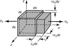
The lateral contraction of a cubic element from a bar in tension is illustrated in Fig. 2.15, where it is assumed that the faces of the element at the origin are fixed in position. From the figure, subsequent to straining, the final volume is
(b)
Figure 2.15. Lateral contraction of an element in tension.
Expanding the right side and neglecting higher-order terms involving ![]() and
and ![]() , we have
, we have
Vf = [1 + (εx – 2νεx)]dx dy dz = Vo + ΔV
where Vo is the initial volume dx dy dz and ΔV is the change in volume. The unit volume change e, also referred to as the dilatation, may now be expressed in the form
(2.29)
Observe from this equation that a tensile force increases and a compressive force decreases the volume of the element.
Example 2.4. Deformation of a Tension Bar
An aluminum alloy bar of circular cross-sectional area A and length L is subjected to an axial tensile force P (Fig. 2.16). The modulus of elasticity and Poisson’s ratio of the material are E and v, respectively. For the bar, determine (a) the axial deformation; (b) the change in diameter d; and (c) the change in volume ΔV. (d) Evaluate the numerical values of the quantities obtained in (a) through (c) for the case in which P = 60 kN, d = 25 mm, L = 3 m, E = 70 GPa, ν = 0.3, and the yield strength σyp = 260 MPa.
Figure 2.16. Example 2.4. A bar under tensile forces.

Solution
If the resulting axial stress σ = P/A does not exceed the proportional limit of the material, we may apply Hooke’s law and write σ = Eε. Also, the axial strain is defined by ε = δ/L.
a. The preceding expressions can be combined to yield the axial deformation,
(2.30)
where the product AE is known as the axial rigidity of the bar.
b. The change in diameter equals the product of transverse or lateral strain and diameter: εtd = –νεd. Thus,
(2.31a)
c. The change in volume, substituting Vo = AL and εx = P/AE into Eq. (2.29), is
(2.31b)
d. For A = (π/4)(252) = 490.9(10–6) m2, the axial stress σ in the bar is obtained from
![]()
which is well below the yield strength of 260 MPa. Thus, introducing the given data into the preceding equations, we have

Comment
A positive sign indicates an increase in length and volume; the negative sign means that the diameter has decreased.
2.10 Generalized Hooke’s Law
For a three-dimensional state of stress, each of the six stress components is expressed as a linear function of six components of strain within the linear elastic range, and vice versa. We thus express the generalized Hooke’s law for any homogeneous elastic material as follows:

(2.32)
The coefficients cij(i, j = 1, 2, 3..., 6) are the material-dependent elastic constants. A succinct representation of the preceding stress–strain relationships are given in the following form:
(2.33)
which is valid in all coordinate systems. Thus, it follows that the cmnij, requiring four subscripts for definition, are components of a tensor of rank 4. We note that, to avoid repetitive subscripts, the material constants c1111, c1122, ..., c6666 are denoted c11, c12, ..., c66, as indicated in Eqs. (2.32).
In a homogeneous body, each of the 36 constants cij has the same value at all points. A material without any planes of symmetry is fully anisotropic. Strain energy considerations can be used to show that for such materials, cij = cji; thus the number of independent material constants can be as large as 21 (see Sec. 2.13). In case of a general orthotropic material, the number of constants reduces to nine, as shown in Section 2.11. For a homogeneous isotropic material, the constants must be identical in all directions at any point. An isotropic material has every plane as a plane of symmetry. Next, it is observed that if the material is isotropic, the number of essential elastic constants reduces to two.
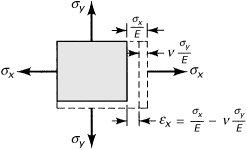
In the following derivation, we rely on certain experimental evidence: a normal stress (σx) creates no shear strain whatsoever, and a shear stress (τxy) creates only a shear strain (γxy). Also, according to the small deformation assumption, the principle of superposition applies under multiaxial stressing. Consider now a two-dimensional homogeneous isotropic rectangular element of unit thickness, subjected to a biaxial state of stress (Fig. 2.17). Were σx to act, not only would the direct strain σx/E but a y contraction would take place as well, –νσx/E. Application of σy alone would result in an x contraction –νσy/E and a y strain σy/E. The simultaneous action of σx and σy, applying the principle of superposition, leads to the following strains:
(a)
Figure 2.17. Element deformations caused by biaxial stresses.
For pure shear (Fig. 1.3c), it is noted in Section 2.9 that, in the linearly elastic range, stress and strain are related by
![]()
Similar analysis enables us to express the components εz, γyz, and γxz of strain in terms of stress and material properties. In the case of a three-dimensional state of stress, this procedure leads to the generalized Hooke’s law, valid for an isotropic homogeneous material:

(2.34)
It is demonstrated next that the elastic constants E, v, and G are related, serving to reduce the number of independent constants in Eq. (2.34) to two. For this purpose, refer again to the element subjected to pure shear (Fig. 1.3c). In accordance with Section 1.9, a pure shearing stress τxy can be expressed in terms of the principal stresses acting on planes (in the x′ and y′ directions) making an angle of 45° with the shear planes: σx′ = τxy and σy′ = –τxy. Then, applying Hooke’s law, we find that
(b)
On the other hand, because εx = εy = 0 for pure shear, Eq. (2.13a) yields, for θ = 45°, εx′ = γxy/2, or
(c)
Equating the alternative relations for εx′ in Eqs. (b) and (c), we find that
(2.35)
It is seen that, when any two of the constants ν, E, and G are determined experimentally, the third may be found from Eq. (2.35). From Eq. (2.34) together with Eq. (2.35), we obtain the following stress–strain relationships:

(2.36)
Here
(2.37)
and
(2.38)
The shear modulus G and the quantity λ are referred to as the Lamé constants. Following a procedure similar to that used for axial stress in Section 2.9, it can be shown that Eq. (2.37) represents the unit volume change or dilatation of an element in triaxial stress.
The bulk modulus of elasticity is another important constant. The physical significance of this quantity is observed by considering, for example, the case of a cubic element subjected to hydrostatic pressure p. Because the stress field is described by σx = σy = σz = –p and τxy = τyz = τxz = 0, Eq. (2.37) reduces to e = –3(1 – 2ν)p/E. The foregoing may be written in the form
(2.39)
where K is the modulus of volumetric expansion or bulk modulus of elasticity. It is seen that the unit volume contraction is proportional to the pressure and inversely proportional to K. Equation (2.39) also indicates that for incompressible materials, for which e = 0, Poisson’s ratio is 1/2. For all common materials, however, ν < 1/2, since they demonstrate some change in volume, e ≠ 0. Table D.1 lists average mechanical properties for a number of common materials. The relationships connecting the elastic constants introduced in this section are given by Eqs. (P2.51) in Prob. 2.51.
Example 2.5. Volume Change of a Metal Block
Calculate the volumetric change of the metal block shown in Fig. 2.18 subjected to uniform pressure p = 160 MPa acting on all faces. Use E = 210 GPa and ν = 0.3.
Figure 2.18. Example 2.5. A parallelpiped under pressure.

Solution
The bulk modulus of elasticity of the material, using Eq. (2.39), is
![]()
![]()
Since the initial volume of the block (Fig. 2.18) is Vo = 2 × 1.5 × 1 = 3 m3, Eq. (2.29) yields
ΔV = eVo = (–9.14 × 10⁻⁴)(3 × 10⁹) = –2.74 × 106 mm3
where a minus sign means that the block experiences a decrease in the volume, as expected intuitively.
2.11 Hooke’s Law for Orthotropic Materials
A general orthotropic material has three planes of symmetry and three corresponding orthogonal axes called the orthotropic axes. Within each plane of symmetry, material properties may be different and independent of direction. A familiar example of such an orthotropic material is wood. Strength and stiffness of wood along its grain and in each of the two perpendicular directions vary. These properties are greater in a direction parallel to the fibers than in the transverse direction. A polymer reinforced by parallel glass or graphite fibers represents a typical orthotropic material with two axes of symmetry.
Materials such as corrugated and rolled metal sheet, reinforced concrete, various composites, gridwork, and particularly laminates can also be treated as orthotropic [Refs. 2.8 and 2.10]. We note that a gridwork consists of two systems of equally spaced parallel ribs (beams), mutually perpendicular and attached rigidly at the points of intersection. For an elastic orthotropic material, the elastic coefficients cij remain invariant at a point under a rotation of 180° about any of the orthotropic axes. In the following derivations, we shall assume that the directions of orthotropic axes are parallel to the directions of the x, y, and z coordinates.*
First, let the xy plane be a plane material symmetry and rotate Oz through 180° (Fig. 2.19a). Accordingly, under the coordinate transformation x: x′, y: y′, and z: –z′, the direction cosines (see Table 1.1) are
(a)
Figure 2.19. Orthotropic coordinates x, y, z: (a) with Oz rotated 180°; (b) with Oy rotated 180°.

Carrying Eqs. (a) into Eqs. (1.28) and (2.18), we have
(b)
and
(c)
Inasmuch as the cij remain the same, the first of Eqs. (2.28) may be written as
(d)
Inserting Eqs. (b) and (c) into Eq. (d) gives
(e)
Comparing Eq. (e) with the first of Eqs. (2.28) shows that c15 = –c15, c16 = –c16, implying that c15 = c16 = 0. Likewise, considering σy′, σz′, τx′y′, τy′z′, τx′z′, we obtain that c25 = c26 = c35 = c36 = c45 = c46 = 0. The elastic coefficient matrix [cij] is therefore
(f)
Next, consider the xz plane of elastic symmetry by rotating Oy through a 180° angle (Fig. 2.19b). This gives l1 = n3 = 1, m2 = –1 and l2 = l3 = m1 = m3 = n1 = n2 = 0. Upon following a procedure similar to that in the preceding, we now obtain c14 = c24 = c34 = c56 = 0. The matrix of elastic coefficients, Eqs. (f), become then

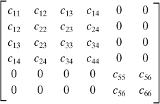
(2.40)
Finally, letting yz be the plane of elastic symmetry and repeating the foregoing procedure do not lead to further reduction in the number of nine elastic coefficients of Eqs. (2.40). Hence, the generalized Hooke’s law for the most general orthotropic elastic material is given by

(2.41)
The inversed form of Eqs. (2.41), referring to Eqs. (2.34), may be expressed in terms of orthotropic moduli and orthotropic Poisson’s ratios as follows:

(2.42)
Because of symmetry in the material constants (Sec. 2.13), we have
(2.43)
In the foregoing, the quantities Ex, Ey, Ez designate the orthotropic moduli of elasticity, and Gxy, Gyz, Gxz are the orthotropic shear moduli in the orthotropic coordinate system. Poisson’s ratio νxy indicates the strain in the y direction produced by the stress in the x direction. The remaining Poisson’s ratios νxz, νyz, ..., νxz are interpreted in a like manner. We observe from Eqs. (2.42) that, in an orthotropic material, there is no interaction between the normal stresses and the shearing strains.
2.12 Measurement of Strain: Strain Rosette
A wide variety of mechanical, electrical, and optical systems has been developed for measuring the normal strain at a point on a free surface of a member [Ref. 2.12]. The method in widest use employs the bonded electric wire or foil resistance strain gages. The bonded wire gage consists of a grid of fine wire filament cemented between two sheets of treated paper or plastic backing (Fig. 2.20a). The backing insulates the grid from the metal surface on which it is to be bonded and functions as a carrier so that the filament may be conveniently handled. Generally, 0.025-mm diameter wire is used. The grid in the case of bonded foil gages is constructed of very thin metal foil (approximately 0.0025 mm) rather than wire. Because the filament cross section of a foil gage is rectangular, the ratio of surface area to cross-sectional area is higher than that of a round wire. This results in increased heat dissipation and improved adhesion between the grid and the backing material. Foil gages are readily manufactured in a variety of configurations. In general, the selection of a particular bonded gage depends on the specific service application.
Figure 2.20. (a) Strain gage (courtesy of Micro-Measurements Division, Vishay Intertechnology, Inc.) and (b) schematic representation of a strain rosette.

The ratio of the unit change in the resistance of the gage to the unit change in length (strain) of the gage is called the gage factor. The metal of which the filament element is made is the principal factor determining the magnitude of this factor. Constantan, an alloy composed of 60% copper and 40% nickel, produces wire or foil gages with a gage factor of approximately 2.
The operation of the bonded strain gage is based on the change in electrical resistance of the filament that accompanies a change in the strain. Deformation of the surface on which the gage is bonded results in a deformation of the backing and the grid as well. Thus, with straining, a variation in the resistance of the grid will manifest itself as a change in the voltage across the grid. An electrical bridge circuit, attached to the gage by means of lead wires, is then used to translate electrical changes into strains. The Wheatstone bridge, one of the most accurate and convenient systems of this type employed, is capable of measuring strains as small as 1 μ.
Strain Rosette
Special combination gages are available for the measurement of the state of strain at a point on a surface simultaneously in three or more directions. It is usual to cluster together three gages to form a strain rosette, which may be cemented on the surface of a member. Generally, these consist of three gages whose axes are either 45° or 60° apart. Consider three strain gages located at angles θa, θb, and θc with respect to reference axis x (Fig. 2.20b). The a-, b-, and c-directed normal strains are, from Eq. (2.13a),
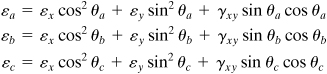
(2.44)
When the values of εa, εb, and εc are measured for given gage orientations θa, θb, and θc the values of εx, εy, and γxy can be obtained by simultaneous solution of Eqs. (2.44). The arrangement of gages employed for this kind of measurement is called a strain rosette.
Once strain components are known, we can apply Eq. (3.11b) of Section 3.4 to determine the out-of-plane principal strain εz. The in-plane principal strains and their orientations may be obtained readily using Eqs. (2.15) and (2.16), as illustrated next, or Mohr’s circle for strain.
Example 2.6. Principal Strains on Surface of a Steel Frame
Strain rosette readings are made at a critical point on the free surface in a structural steel member. The 60° rosette contains three wire gages positioned at 0°, 60°, and 120° (Fig. 2.20b). The readings are
(a)
Determine (a) the in-plane principal strains and stresses and their directions, and (b) the true maximum shearing strain. The material properties are E = 200 GPa and ν = 0.3.
Solution
For the situation described, Eq. (2.44) provides three simultaneous expressions:


(b)
Note that the relationships among εa, εb, and εc may be observed from a Mohr’s circle construction corresponding to the state of strain εx, εy, and γxy at the point under consideration.
a. Upon substituting numerical values, we obtain εx = 190 μ, εy = –130 μ, and γxy = 577 μ. Then, from Eq. (2.16), the principal strains are
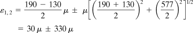
or
(c)
The maximum shear strain is found from
γmax = ±(ε1 – ε2) = ±[360 – (–300)]μ = ±660 μ
The orientations of the principal axes are given by Eq. (2.15):
(d)
When ![]() is substituted into Eq. (2.14) together with Eq. (b), we obtain 360 μ. Therefore, 30.5° and 120.5° are the respective directions of ε1 and ε2, measured from the horizontal axis in a counterclockwise direction. The principal stresses may now be found from the generalized Hooke’s law. Thus, the first two equations of (2.34) for plane stress, letting σz = 0, σx = σ1, and σy = σ2, together with Eqs. (c), yield
is substituted into Eq. (2.14) together with Eq. (b), we obtain 360 μ. Therefore, 30.5° and 120.5° are the respective directions of ε1 and ε2, measured from the horizontal axis in a counterclockwise direction. The principal stresses may now be found from the generalized Hooke’s law. Thus, the first two equations of (2.34) for plane stress, letting σz = 0, σx = σ1, and σy = σ2, together with Eqs. (c), yield

The directions of σ1 and σ2 are given by Eq. (d). From Eq. (2.36), the maximum shear stress is
![]()
Note as a check that (σ1 – σ2)/2 yields the same result.
b. Applying Eq. (3.11b), the out-of-plane principal strain is
![]()
The principal strain ε2 found in part (a) is redesignated ε3 = –300 μ so that algebraically ε2 > ε3, where ε2 = –26 μ. The true or absolute maximum shearing strain
(2.45)
is therefore ±660 μ, as already calculated in part (a).
Employing a procedure similar to that used in the preceding numerical example, it is possible to develop expressions relating three-element gage outputs of various rosettes to principal strains and stresses. Table 2.2 provides two typical cases: equations for the rectangular rosette (θa = 0°, θb = 45°, and θc = 90°, Fig. 2.20b) and the delta rosette (θa = 0°, θb = 60°, and θc = 120°, Fig. 2.20b). Experimental stress analysis is facilitated by this kind of compilation.
Table 2.2. Strain Rosette Equations
1. Rectangular rosette or 45° strain rosette
Principal strains:
(2.46a)
Principal stresses:
(2.46b)
Directions of principal planes:
(2.46c)
2. Delta rosette or 60° strain rosette
Principal strains:
(2.47a)
Principal stresses:
(2.47b)
Directions of principal planes:

(2.47c)
2.13 Strain Energy
The work done by external forces in causing deformation is stored within the body in the form of strain energy. In an ideal elastic process, no dissipation of energy takes place, and all the stored energy is recoverable upon unloading. The concept of elastic strain energy, introduced in this section, is useful as applied to the solution of problems involving both static and dynamic loads. It is particularly significant for predicting failure in members under combined loading.
Strain Energy Density for Normal and Shear Stresses
We begin our analysis by considering a rectangular prism of dimensions dx, dy, dz subjected to uniaxial tension. The front view of the prism is represented in Fig. 2.21a. If the stress is applied very slowly, as is generally the case in this text, it is reasonable to assume that equilibrium is maintained at all times. In evaluating the work done by stresses σx on either side of the element, it is noted that each stress acts through a different displacement. Clearly, the work done by oppositely directed forces (σx dy dz) through positive displacement (u) cancel one another. The net work done on the element by force (σx dy dz) is therefore
![]()
Figure 2.21. (a) Displacement under uniaxial stress; (b) work done by uniaxial stress.
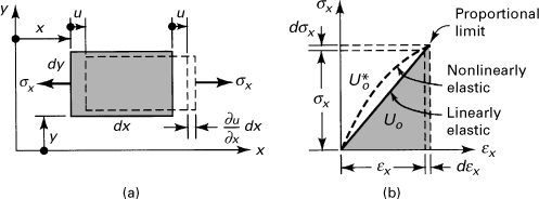
where ∂u/∂x = εx. Note that dW is the work done on dx dy dz, and dU is the corresponding increase in strain energy. Designating the strain energy per unit volume (strain energy density) as Uo, for a linearly elastic material we have
(a)
After integration, Eq. (a) yields
(2.48)
This quantity represents the shaded area in Fig. 2.21b. The area above the stress–strain curve, termed the complementary energy density, may be determined from

(2.49)
For a linearly elastic material, ![]() but for a nonlinearly elastic material, Uo and
but for a nonlinearly elastic material, Uo and ![]() will differ, as seen in the figure. The unit of strain energy density in SI units is the joules per cubic meter (J/m3), or pascals; in U.S. Customary Units, it is expressed in inch-pounds per cubic inch (in. · lb/in.3), or pounds per square inch (psi).
will differ, as seen in the figure. The unit of strain energy density in SI units is the joules per cubic meter (J/m3), or pascals; in U.S. Customary Units, it is expressed in inch-pounds per cubic inch (in. · lb/in.3), or pounds per square inch (psi).
When the material is stressed to the proportional limit, the strain energy density is referred to as the modulus of resilience. It is equal to the area under the straight-line portion of the stress–strain diagram (Fig. 2.10a) and represents a measure of the material’s ability to store or absorb energy without permanent deformation. Similarly, the area under an entire stress–strain diagram provides a measure of a material’s ability to absorb energy up to the point of fracture; it is called the modulus of toughness. The greater the total area under a stress–strain diagram, the tougher the material.
In the case in which σx, σy, and σz act simultaneously, the total work done by these normal stresses is simply the sum of expressions similar to Eq. (2.48) for each direction. This is because an x-directed stress does no work in the y or z directions. The total strain energy per volume is thus
(b)
The elastic strain energy associated with shear deformation is now analyzed by considering an element of thickness dz subject only to shearing stresses τxy (Fig. 2.22). From the figure, we note that shearing force τxy dxdz causes a displacement of γxy dy. The strain energy due to shear is ![]() , where the factor
, where the factor ![]() arises because the stress varies linearly with strain from zero to its final value, as before. The strain energy density is therefore
arises because the stress varies linearly with strain from zero to its final value, as before. The strain energy density is therefore
Figure 2.22. Deformation due to pure shear.

(2.50)
Because the work done by τxy accompanying perpendicular strains γyz and γxz is zero, the total strain energy density attributable to shear alone is found by superposition of three terms identical in form with Eq. (2.50):
(c)
Strain Energy Density for Three-Dimensional Stresses
Given a general state of stress, the strain energy density is found by adding Eqs. (b) and (c):
(2.51)
Introducing Hooke’s law into Eq. (2.51) leads to the following form involving only stresses and elastic constants:

(2.52)
An alternative form of Eq. (2.51), written in terms of strains, is
(2.53)
The quantities λ and e are defined by Eqs. (2.38) and (2.37), respectively.
It is interesting to observe that we have the relationships
(2.54)
Here Uo(τ) and Uo(ε) designate the strain energy densities expressed in terms of stress and strain, respectively [Eqs. (2.52) and (2.53)]. Derivatives of this type will be discussed again in connection with energy methods in Chapter 10. We note that Eqs. (2.54) and (2.32) give

(2.55)
Differentiations of these equations as indicated result in

(2.56)
We are led to conclude from these results that cij = cji(i, j = 1, 2, ..., 6). Because of this symmetry of elastic constants, there can be at most [(36 – 6)/2] + 6 = 21 independent elastic constants for an anisotropic elastic body.
2.14 Strain Energy in Common Structural Members
To determine the elastic strain energy stored within an entire body, the elastic energy density is integrated over the original or undeformed volume V. Therefore,
(2.57)
The foregoing shows that the energy-absorbing capacity of a body (that is, the failure resistance), which is critical when loads are dynamic in character, is a function of material volume. This contrasts with the resistance to failure under static loading, which depends on the cross-sectional area or the section modulus.
Equation (2.57) permits the strain energy to be readily evaluated for a number of commonly encountered geometries and loadings. Note especially that the strain energy is a nonlinear (quadratic) function of load or deformation. The principle of superposition is thus not valid for the strain energy. That is, the effects of several forces (or moments) on strain energy are not simply additive, as demonstrated in Example 2.7. Some special cases of Eq. (2.57) follow.
Strain Energy for Axially Loaded Bars
The normal stress at any given transverse section through a nonprismatic bar subjected to an axial force P is σx = P/A, where A represents the cross-sectional area (Fig. 2.23). Substituting this and Eq. (2.48) into Eq. (2.57) and setting dV = A dx, we have
(2.58)
Figure 2.23. Nonprismatic bar with varying axial loading.

When a prismatic bar is subjected at its ends to equal and opposite forces of magnitude P, the foregoing becomes
(2.59)
where L is the length of the bar.
Example 2.7. Strain Energy in a Bar under Combined Loading
A prismatic bar suspended from one end carries, in addition to its own weight, an axial load Po (Fig. 2.24). Determine the strain energy U stored in the bar.
Figure 2.24. Example 2.7. A prismatic bar loaded by its weight and load Po.

Solution
The axial force P acting on the shaded element indicated is expressed
(a)
where γ is the specific weight of the material and A, the cross-sectional area of the bar. Inserting Eq. (a) into Eq. (2.58), we have

(2.60)
The first and the third terms on the right side represent the strain energy of the bar subjected to its own weight and the strain energy of a bar supporting only axial force Po respectively. The presence of the middle term indicates that the strain energy produced by the two loads acting simultaneously is not simply equal to the sum of the strain energies associated with the loads acting separately.
Strain Energy of Circular Bars in Torsion
Consider a circular bar of varying cross section and varying torque along its axis (Fig. 2.23, with double-headed torque vector T replacing force vector P). The state of stress is pure shear. The torsion formula (Table 1.1) for an arbitrary distance ρ from the centroid of the cross section results in τ = Tρ/J. The strain energy density, Eq. (2.50), becomes then Uo = T2ρ2/2J2G. When this is introduced into Eq. (2.57), we obtain
(b)
where dV = dA dx; dA represents the cross-sectional area of an element. By definition, the term in parentheses is the polar moment of inertia J of the cross-sectional area. The strain energy is therefore
(2.61)
In the case of a prismatic shaft subjected at its ends to equal and opposite torques T, Eq. (2.61) yields
(2.62)
where L is the length of the bar.
Strain Energy for Beams in Bending
For the case of a beam in pure bending, the flexure formula gives us the axial normal stress σx = –My/I (see Table 1.1). From Eq. (2.48), the strain energy density is Uo = M2y2/2EI2. Upon substituting this into Eq. (2.57) and noting that M2/2EI2 is a function of x alone, we have
(c)
Here, as before, dV = dA dx, and dA represents an element of the cross-sectional area. Recalling that the integral in parentheses defines the moment of inertia I of the cross-sectional area about the neutral axis, the strain energy is expressed as
(2.63)
where integration along beam length L gives the required quantity.
2.15 Components of Strain Energy
A new perspective on strain energy may be gained by viewing the general state of stress (Fig. 2.25a) in terms of the superposition shown in Fig. 2.25. The state of stress in Fig. 2.25b, represented by
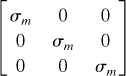
(a)
Figure 2.25. Resolution of (a) state of stress into (b) dilatational stresses and (c) distortional stresses.
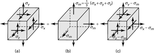
results in volume change without distortion and is termed the dilatational stress tensor. Here ![]() is the mean stress defined by Eq. (1.44). Associated with σm is the mean strain,
is the mean stress defined by Eq. (1.44). Associated with σm is the mean strain, ![]() . The sum of the normal strains accompanying the application of the dilatational stress tensor is the dilatation e = εx + εy + εz, representing a change in volume only. Thus, the dilatational strain energy absorbed per unit volume is given by
. The sum of the normal strains accompanying the application of the dilatational stress tensor is the dilatation e = εx + εy + εz, representing a change in volume only. Thus, the dilatational strain energy absorbed per unit volume is given by
(2.64)
where K is defined by Eq. (2.39).
The state of stress in Fig. 2.25c, represented by
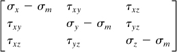
(b)
is called the deviator or distortional stress tensor. This produces deviator strains or distortion without change in volume because the sum of the normal strains is (εx – εm) + (εy – εm) + (εz – εm) = 0. The distortional energy per unit volume, Uod, associated with the deviator stress tensor is attributable to the change of shape of the unit volume, while the volume remains constant. Since Uov and Uod are the only components of the strain energy, we have Uo = Uov + Uod. By subtracting Eq. (2.64) from Eq. (2.52), the distortional energy is readily found to be
(2.65)
This is the elastic strain energy absorbed by the unit volume as a result of its change in shape (distortion). In the preceding, the octahedral shearing stress τoct is given by
(2.66)
The planes where the τoct acts are shown in Fig. 1.24 of Section 1.14. The strain energy of distortion plays an important role in the theory of failure of a ductile metal under any condition of stress. This is discussed further in Chapter 4. The stresses and strains associated with both components of the strain energy are also very useful in describing the plastic deformation (Chap. 12).
Example 2.8. Strain Energy Components in a Tensile Bar
A mild steel bar of uniform cross section A is subjected to an axial tensile load P. Derive an expression for the strain energy density, its components, and the total strain energy stored in the bar. Let ν = 0.25.
Solution
The state of stress at any point in the bar is axial tension, τxy = τxz = τyz = σy = σz = 0, σx = σ = P/A (Fig. 2.25a). We therefore have the stresses associated with volume change σm = σ/3 and shape change σx – σm = 2σ/3, σy – σm = σz – σm = –σ/3 (Fig. 2.25b, c). The strain energy densities for the state of stress in cases a, b, and c are found, respectively, as follows:
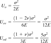
(c)
Observe from these expressions that Uo = Uov + Uod and that 5Uov = Uod. Thus, we see that in changing the shape of a unit volume element under uniaxial stressing, five times more energy is absorbed than in changing the volume.
2.16 Saint-Venant’s Principle
The reader will recall from a study of Newtonian mechanics that, for purposes of analyzing the statics or dynamics of a body, one force system may be replaced by an equivalent force system whose force and moment resultants are identical. It is often added in discussing this point that the force resultants, while equivalent, need not cause an identical distribution of strain, owing to difference in the arrangement of the forces. Saint-Venant’s principle, named for Barré de Saint-Venant (1797–1886), a famous French mathematician and elastician, permits the use of an equivalent loading for the calculation of stress and strain. This principle or rule states that if an actual distribution of forces is replaced by a statically equivalent system, the distribution of stress and strain throughout the body is altered only near the regions of load application.*
The contribution of Saint-Venant’s principle to the solution of engineering problems is very important, for it often frees the analyst of the burden of prescribing the boundary conditions very precisely when it is difficult to do so. Furthermore, where a certain solution is predicated on a particular boundary loading, the solution can serve equally for another type of statically equivalent boundary loading, not quite the same as the first. That is, when an analytical solution calls for a certain distribution of stress on a boundary (such as σx in Sec. 5.5), we need not discard the solution merely because the boundary distribution is not quite the same as that required by the solution. The value of existing solutions is thus greatly extended.
Saint-Venant’s principle is confirmed in Fig. 2.26, which shows the stress distribution, obtained using the methods of the theory of elasticity, across three sections of a rectangular elastic plate of width b subjected to a concentrated load [Ref. 2.15]. The average stress σavg as given by Eq. (1.10) is also sketched in the diagrams. From these, note that the maximum stress σmax greatly exceeds the average stress near the point of application of the load and diminishes as we move along the vertical center axis of the plate away from an end. At a distance equal to the width of the plate, the stress is nearly uniform. With rare exceptions, this rule applies to members made of linearly elastic materials.
Figure 2.26. Stress distribution due to a concentrated load in a rectangular elastic plate, confirming the Saint-Venant’s principle.
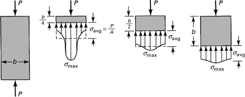
The foregoing observation also holds true for most stress concentrations and practically any type of loading. Thus, the basic formulas of the mechanics of materials give the stress in a member with high accuracy, provided that the cross section in question is at least a distance b (or h) away from any concentrated load or discontinuity of shape. Here, b (or h) denotes the largest lateral dimension of a member. We note that within this distance the stresses depend on the details of loading, boundary conditions, and geometry of the stress concentrations, as is seen in Chapter 3.
Consider, for example, the substitution of a uniform distribution of stress at the ends of a tensile test specimen for the actual irregular distribution that results from end clamping. If we require the stress in a region away from the ends, the stress variation at the ends need not be of concern, since it does not lead to significant variation in the region of interest. As a further example, according to Saint-Venant’s principle, the complex distribution of force supplied by the wall to a cantilever beam (Fig. 2.27a) may be replaced by vertical and horizontal forces and a moment (Fig. 2.27b) for purposes of determining the stresses acting at a distance from the wall equal to or greater than the depth h of the beam.
Figure 2.27. Cantilever beam illustrating use of Saint-Venant’s principle: (a) actual support; (b) statical equivalent.

References
2.1. SOKOLNIKOFF, I. S., Mathematical Theory of Elasticity, 2nd ed., Krieger, Melbourne, Fla., 1986.
2.2. CHOU, P. C., and PAGANO, N. J., Elasticity, Dover, New York, 1992.
2.3. FLUGGE, W., ed., Handbook of Engineering Mechanics, McGraw-Hill, New York, 1962, Chap. 2.
2.4. BORESI, A. P., and SCHMIDT, R. J., Advanced Mechanics of Materials, 6th ed., Wiley, Hoboken, N.J., 2003, Chap. 2.
2.5. AVALLONE, E. A., and BAUMEISTER III, T., eds., Mark’s Standard Handbook for Mechanical Engineers, 10th ed., McGraw-Hill, New York, 1997.
2.6. American Society of Testing and Materials, Annual Book of ASTM, Philadelphia, Pa, 2009.
2.7. UGURAL, A. C., Mechanical Design: An Integrated Approach, McGraw-Hill, New York, 2004.
2.8. FAUPEL, J. H., and FISHER, F. E., Engineering Design, 2nd ed., Wiley, Hoboken, N.J., 1981.
2.9. UGURAL, A.C., Mechanics of Materials, Wiley, Hoboken, N.J., 2008.
2.10. UGURAL, A. C., Stresses in Beams, Plates, and Shells, CRC Press, Taylor & Francis Group, Boca Raton, Fla., 2010.
2.11. SHAMES, I. H., and COZZARELLI, F. A., Elastic and Inelastic Stress Analysis, Prentice Hall, Englewood Cliffs, N.J., 1992.
2.12. HETENYI, M., ed., Handbook of Experimental Stress Analysis, 2nd ed., Wiley, Hoboken, N.J., 1987.
2.13. STERNBERG, E., On St. Venant’s principle. Quart. Appl. Math. 11:393, 1954.
2.14. STERNBERG, E., and KOTTER, T., The wedge under a concentrated couple, J. Appl., Mech. 25-575-581, 1958.
2.15. TIMOSHENKO, S. P., and GOODIER, J. N., Theory of Elasticity, 3rd ed., McGraw Hill, New York, 1970, p. 60.
Problems
Sections 2.1 through 2.8
2.1. Determine whether the following strain fields are possible in a continuous material:
a. ![]() ,
,
b. ![]()
Here c is a small constant, and it is assumed that εz = γxz = γyz = 0.
2.2. Rectangle ABCD is scribed on the surface of a member prior to loading (Fig. P2.2). Following the application of the load, the displacement field is expressed by
![]()

where c = 10–4. Subsequent to the loading, determine (a) the length of the sides AB and AD; (b) the change in the angle between sides AB and AD; and (c) the coordinates of point A.
2.3. A displacement field in a body is given by
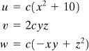
where c = 10–4. Determine the state of strain on an element positioned at (0, 2, 1).
2.4. The displacement field and strain distribution in a member have the form
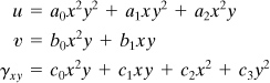
What relationships connecting the constants (a’s, b’s, and c’s) make the foregoing expressions possible?
2.5. Redo Prob. 2.4 for the following system of strains:
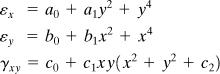
2.6. A rigid horizontal bar BE is supported as illustrated in Fig. P2.6. After the load P is applied, point E moves 3 mm down and the axial strain in the bar AB is –500 μ. Calculate the axial strain in the bar CD.

2.7. Find the normal strain in the members AB and CB of the pin-connected plane structure (Fig. P2.7) if point B is moved leftward 2.5 mm. Assume that axial deformation is uniform throughout the length of each member.

2.8. The thin, triangular plate ABC is uniformly deformed into a shape ABC as depicted by the dashed lines in Fig. P2.8. Determine (a) the plane stress components εx, εy, and γxy; (b) the shearing strain between edges AC and BC.

2.9. A 100-mm by 150-mm rectangular plate QABC is deformed into the shape shown by the dashed lines in Fig. P2.9. All dimensions shown in the figure are in millimeters. Determine at point Q (a) the strain components εx, εy, γxy, and (b) the principal strains and the direction of the principal axes.
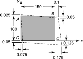
2.10. Calculate the principal strains and their orientations at point A of the deformed rectangular plate shown in Fig. 2.5 of Example 2.1.
2.11. As a result of loading, the rectangle shown in Fig. P2.11 deforms into a parallelogram in which sides QA and BC shorten 0.003 mm and rotate 500 μ radian counterclockwise while sides AB and QC elongate 0.004 mm and rotate 1000 μ radian clockwise. Determine the principal strains and the direction of the principal axes at point Q. Take a = 20 mm and b = 12mm.

2.12. A thin rectangular plate a = 20 mm × b = 12 mm (Fig. P2.11) is acted upon by a stress distribution resulting in the uniform strains εx = 300 μ, εy = 500 μ, and γxy = 200 μ. Determine the changes in length of diagonals QB and AC.
2.13. Redo Prob. 2.12 using the following information: a = 30 mm, b = 15 mm, εx = 400 μ, εy = 200 μ, and γxy = –300 μ.
2.14. A thin plate is subjected to uniform shear stress τo = 70 MPa (Fig. P1.42 of Chap. 1). Let E = 200 GPa, ν = 0.3, AB = 40 mm, and BC = 60 mm. Determine (a) the change in length AB, (b) the changes in length of diagonals AC and BD, and (c) the principal strains and their directions at point A.
2.15. The principal strains at a point are ε1 = 400 μ and ε2 = 200 μ. Determine (a) the maximum shear strain and the direction along which it occurs and (b) the strains in the directions at θ = 30° from the principal axes. Solve the problem by using the formulas developed and check the results by employing Mohr’s circle.
2.16. A 3-m by 2-m rectangular thin plate is deformed by the movement of point B to B′ as shown by the dashed lines in Fig. P2.16. Assuming a displacement field of the form u = c1xy and v = c2xy, wherein c1 and c2 are constants, determine (a) expressions for displacements u and v; (b) strain components εx, εy, and γxy at point B; and (c) the normal strain εx′ in the direction of line QB. Verify that the strain field is possible.

2.17. If the strains at a point are εx = –900 μ, εy = –300 μ, and γxy = 900 μ, what are the principal strains, and in what direction do they occur? Use Mohr’s circle of strain.
2.18. Solve Prob. 2.17 for εx = 300 μ, εy = 900 μ, and γxy = –900 μ.
2.19. A 3-m by 1-m by 2-m parallelepiped is deformed by movement of corner A to A′ (2.9995, 1.0003, 1.9994), as shown in Fig. P2.19. Assuming that the displacement field is given by Eqs. (2.22), calculate at point A (a) the strain components and ascertain whether this strain distribution is possible; (b) the normal strain in the direction of line AB; and (c) the shearing strain for the perpendicular lines AB and AC.

2.20. Redo Prob. 2.19 for the case in which corner point A is moved to A′ (3.0006, 0.9997, 1.9996).
2.21. At a point in a stressed body, the strains, related to the coordinate set xyz, are given by
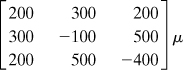
Determine (a) the strain invariants; (b) the normal strain in the x′ direction, which is directed at an angle θ = 30° from the x axis; (c) the principal strains ε1, ε2, and ε3; and (d) the maximum shear strain.
2.22. Solve Prob. 2.21 for a state of strain given by
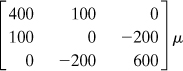
2.23. The following describes the state of strain at a point in a structural member:

Determine the magnitudes and directions of the principal strains.
2.24. A tensile test is performed on a 12-mm-diameter aluminum alloy specimen (ν = 0.33) using a 50-mm gage length. When an axial tensile load reaches a value of 16 kN, the gage length has increased by 0.10 mm. Determine (a) the modulus of elasticity; (b) the decrease Δd in diameter and the dilatation e of the bar.
2.25. A 12-mm-diameter specimen is subjected to tensile loading. The increase in length resulting from a load of 9 kN is 0.025 mm for an original length Lo of 75 mm. What are the true and conventional strains and stresses? Calculate the modulus of elasticity.
Sections 2.9 through 2.12
2.26. Find the smallest diameter and shortest length that may be selected for a steel control rod of a machine under an axial load of 5 kN if the rod must stretch 2 mm. Use E = 210 GPa and σall = 160 MPa.
2.27. A 40-mm diameter bar ABC is composed of an aluminum part AB and a steel part BC (Fig. P2.27). After axial force P is applied, a strain gage attached to the steel measures normal strain at the longitudinal direction as εs = 600 μ. Determine (a) the magnitude of the applied force P; (b) the total elongation of the bar if each material behaves elastically. Take Ea = 70 GPa and Es = 210 GPa.

2.28. A 5-m-long truss member is made of two 40-mm-diameter steel bars. For a tensile load of 600 kN, find (a) the change in the length of the member; (b) the change in the diameter of the member. Use E = 200 GPa, σyp = 250 MPa, and ν = 0.3.
2.29. The cast-iron pipe of length L, outer diameter D, and thickness t is subjected to an axial compressive P. Calculate (a) the change in length ΔL; (b) the change in outer diameter D; (c) the change in thickness Δt. Given: D = 100 mm, t = 10 mm, L = 0.4 m, P = 150 kN, E = 70 GPa, and ν = 0.3.
2.30. A typical vibration isolation device consists of rubber cylinder of diameter d compressed inside of a steel cylinder by a force Q applied to a steel rod, as schematically depicted in Fig. P2.30. Find, in terms of d, Q, and Poisson’s ratio ν for the rubber, as needed: (a) an expression for the lateral pressure p between the rubber and the steel cylinder; (b) the lateral pressure p between the rubber and the steel cylinder for d = 50 mm, ν = 0.3, and Q = 5 kN. Assumptions: 1. Friction between the rubber and steel can be neglected; 2. Steel cylinder and rod are rigid.

2.31. A solid sphere of diameter d experiences a uniform pressure of p. Determine (a) the decrease in circumference of the sphere; (b) the decrease in volume of the sphere ΔV. Given: d = 250 mm, p = 160 MPa, E = 70 GPa, and ν = 0.3. Note: Volume of a sphere is ![]() , where r = d/2.
, where r = d/2.
2.32. The state of strain at a point in a thin steel plate is εx = 500 μ, εy = –100 μ, and γxy = 150 μ. Determine (a) the in-plane principal strains and the maximum in-plane shear strain; (b) true maximum shearing strain ν = 0.3. Sketch the results found in part (a) on properly oriented deformed elements.
2.33. An element at a point on a loaded frame has strains as follows: εx = 480 μ, εy = 800 μ and γxy = –1120 μ. Determine (a) the principal strains; (b) the maximum shear strain; (c) the true maximum shearing strain.
2.34. A metallic plate of width w and thickness t is subjected to a uniform axial force P as shown in Fig. P2.34. Two strain gages placed at point A measure the strains εx′ and at 30° and 60°, respectively, to the axis of the plate. Calculate (a) the normal strains εx and εy; (b) the normal strains εx′ and εy′; (c) the shearing strain γx′y′. Given: w = 60 mm, t = 6 mm, E = 200 GPa, ν = 0.3, and P = 25 kN.
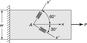
2.35. During the static test of a panel, a 45° rosette reads the following normal strains on the free surface (Fig. P2.35): εa = –800 μ, εb = –1000 μ, and εc = 400 μ. Find the principal strains and show the results on a properly oriented deformed element.


2.36. A 50-mm-square plate is subjected to the stresses shown in Fig. P2.36. What deformation is experienced by diagonal BD? Express the solution, in terms of E, for ν = 0.3 using two approaches: (a) determine the components of strain along the x and y directions and then employ the equations governing the transformation of strain; (b) determine the stress on planes perpendicular and parallel to BD and then employ the generalized Hooke’s law.
2.37. A uniform pressure p acts over the entire straight edge of a large plate (Fig. P2.37). What are normal stress components σx and σz acting on a volumetric element at some distance from the loading in terms of Poisson’s ratio ν and p, as required? Assume that εx = εz = 0 and σy = –p everywhere.

2.38. A 45° rosette is used to measure strain at a critical point on the surface of a loaded beam. The readings are εa = –100 μ, εb = 50 μ, εc = 100 μ for θa = 0°, θb = 45°, and θc = 90° (Fig. 2.20b). Calculate the principal strains and stresses and their directions. Use E = 200 GPa and ν = 0.3.
2.39. The following state of strain has been measured at a point on the surface of a crane hook: εa = 1000 μ, εb = –250 μ, and εc = 200 μ for θa = –15°, θb = 30°, and θc = 75° (Fig. 2.20b). Determine strain components εx, εy, and γxy.
2.40. The strains measured at a point on the surface of a machine element are εa = 400 μ, εb = 300 μ, and εc = –50 μ for θa= 30°, θb = –30°, and θc = 90° (Fig. 2.20b). Calculate (a) the in-plane maximum shearing strain, and (b) the true maximum shearing strain. Use ![]() .
.
2.41. For a given steel, E = 200 GPa and G = 80 GPa. If the state of strain at a point within this material is given by
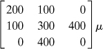
ascertain the corresponding components of the stress tensor.
2.42. For a material with G = 80 GPa and E = 200 GPa, determine the strain tensor for a state of stress given by
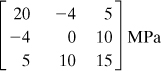
2.43. The distribution of stress in an aluminum machine component is given (in megapascals) by
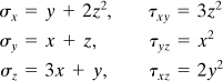
Calculate the state of strain of a point positioned at (1, 2, 4). Use E = 70 GPa and ν = 0.3.
2.44. The distribution of stress in a structural member is given (in megapascals) by Eqs. (d) of Example 1.2 of Chapter 1. Calculate the strains at the specified point ![]() for E = 200 GPa and ν = 0.25.
for E = 200 GPa and ν = 0.25.
2.45. An aluminum alloy plate (E = 70 GPa, ν = 1/3) of dimensions a = 300 mm, b = 400 mm, and thickness t = 10 mm is subjected to biaxial stresses as shown in Fig. P2.45. Calculate the change in (a) the length AB; (b) the volume of the plate.
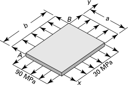
2.46. The steel rectangular parallelepiped (E = 200 GPa and ν = 0.3) shown in Fig. P2.46 has dimensions a = 250 mm, b = 200 mm, and c = 150 mm. It is subjected to triaxial stresses σx = –60 MPa, σy = –50 MPa, and σz = –40 MPa acting on the x, y, and z faces, respectively. Determine (a) the changes Δa, Δb, and Δc in the dimensions of the block, and (b) the change ΔV in the volume.

2.47. Redo Prob. 2.46 for an aluminum block (E = 70 GPa and ![]() ) for which a = 150 mm, b = 100 mm, and c = 75 mm, subjected to stresses σx = 70 MPa, σy = –30 MPa, and σz = –15 MPa.
) for which a = 150 mm, b = 100 mm, and c = 75 mm, subjected to stresses σx = 70 MPa, σy = –30 MPa, and σz = –15 MPa.
2.48. At a point in an elastic body, the principal strains ε3, ε2, ε1 are in the ratio 3: 4: 5; the largest principal stress is σ1 = 140 MPa. Determine the ratio σ3: σ2: σ1 and the values of σ2 and σ3. Take ν = 0.3 and E = 200 GPa.
2.49. A rectangular plate is subjected to uniform tensile stress σ along its upper and lower edges, as shown in Fig. P2.49. Determine the displacements u and ν in terms of x, y, and material properties (E, ν): (a) using Eqs. (2.3) and the appropriate conditions at the origin; (b) by the mechanics of materials approach.

2.50. The stress field in an elastic body is given by
![]()
where c is a constant. Derive expressions for the displacement components u(x, y) and v(x, y) in the body.
2.51. Derive the following relations involving the elastic constants:

(P2.51)
2.52. As shown in Fig. P2.52, a thin prismatical bar of specific weight γ and constant cross section hangs in the vertical plane. Under the effect of its own weight, the displacement field is described by
![]()
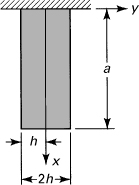
The z displacement and stresses may be neglected. Find the strain and stress components in the bar. Check to see whether the boundary conditions [Eq. (1.48)] are satisfied by the stresses found.
2.53. A uniform bar of rectangular cross section 2h × b and specific weight γ hangs in the vertical plane (Fig. P2.53). Its weight results in displacements

Demonstrate whether this solution satisfies the 15 equations of elasticity and the boundary conditions.

Sections 2.13 through 2.16
2.54. A bar of uniform cross-sectional area A, modulus of elasticity E, and length L is fixed at its right end and subjected to axial forces P1 and P2 at its free end. Verify that the total strain energy stored in the bar is given by
(P2.54)
Note that U is not the sum of the strain energies due to P1 and P2 acting separately. Find the components of the energy for P1 = P2 = P and ν = 0.25.
2.55. Three bars of successively larger volume are to support the same load P (Fig. P2.55). Note that the first bar has a uniform cross-sectional area A over its length L. Neglecting stress concentrations, compare the strain energy stored in the three bars.

2.56. A solid bronze sphere (E = 110 GPa, ![]() , r = 150 mm) is subjected to hydrostatic pressure p so that its volume is reduced by 0.5%. Determine (a) the pressure p, and (b) the strain energy U stored in the sphere. (Note: volume of a sphere
, r = 150 mm) is subjected to hydrostatic pressure p so that its volume is reduced by 0.5%. Determine (a) the pressure p, and (b) the strain energy U stored in the sphere. (Note: volume of a sphere ![]() .)
.)
2.57. Calculate the total strain energy U stored in the block described in Prob. 2.46.
2.58. A round bar is composed of three segments of the same material (Fig. P2.58). The diameter is d for the lengths BC and DE and nd for length CD, where n is the ratio of the two diameters. Neglecting the stress concentrations, verify that the strain energy of the bar when subjected to axial load P is
(P2.58)
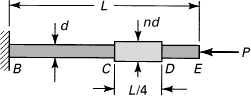
where A = πd2/4. Compare the result for n = 1 with those for ![]() and n = 2.
and n = 2.
2.59. (a) Taking into account only the effect of normal stress, determine the strain energy of prismatic beam AB due to the axial force P and moment Mo acting simultaneously (Fig. P2.59). (b) Evaluate the strain energy for the case in which the beam is rectangular, 100-mm deep by 75-mm wide, P = 8 kN, Mo = 2 kN · m, L = 1.2 m, a = 0.3 m, b = 0.9 m, and E = 70 GPa.
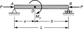
2.60. A stepped shaft is subjected to pure torsion, as shown in Fig. P2.60. Neglecting the stress concentrations, develop the following equation for energy stored in the shaft:
(P2.60)

Here φ is the angle of twist and G represents the modulus of rigidity.
2.61. (a) Determine the strain energy of a solid brass circular shaft ABC loaded as shown in Fig. P2.61, assuming that the stress concentrations may be omitted. (b) Calculate the strain energy for T = 1.4 kN · m, a = 500 mm, d = 20 mm, and G = 42 GPa.

2.62. Consider a simply supported rectangular beam of depth h, width b, and length L subjected to a uniform load of intensity p. Verify that the maximum strain energy density equals
(P2.62)
in which U is the strain energy of the beam and V its volume.
2.63. Consider a beam with simple supports at B and C and an overhang AB (Fig. P2.63). What is the strain energy in the beam due to the load P?
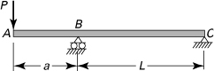
2.64. A simply supported beam carries a concentrated force P and a moment Mo as shown in Fig. P2.64. How much strain energy is stored in the beam owing to the loads acting simultaneously?

2.65. Consider the state of stress given in Fig. 1.20b. Determine how many times more energy is absorbed in changing the shape than in changing the volume of a unit element. Let E = 200 GPa and ν = 0.3.
2.66. The state of stress at a point is

Decompose this array into a set of dilatational stresses and a set of deviator stresses. Determine the values of principal deviator stress.
2.67. Calculate the strain energy per unit volume in changing the volume and in changing the shape of the material at any point on the surface of a steel shaft 120 mm in diameter subjected to torques of 20 kN · m and moments of 15 kN · m at its ends. Use E = 200 GPa and ν = 0.25.
2.68. The state of stress at a point in a loaded member is represented in Fig. P2.68. Express the dilatational energy density and the distortional energy density in terms of the given stresses (σ, τ) at the point and the material properties (E, ν).

2.69. A circular prismatic cantilever is subjected to a torque T and an axial force P at its free end. The length of the bar is L, the radius is r, and the modulus of elasticity of the material is E. Determine the total strain energy stored in the bar and its components. Assume ![]() for the material.
for the material.