Chapter 7. Numerical Methods
7.1 Introduction
This chapter is subdivided into two parts. The finite difference method is treated briefly first. Then, the most commonly employed numerical technique, the finite element method, is discussed. We shall apply both approaches to the solution of problems in elasticity and the mechanics of materials. The use of these numerical methods enables the engineer to expand his or her ability to solve practical design problems. The engineer may now treat real shapes as distinct from the somewhat limited variety of shapes amenable to simple analytic solution. Similarly, the engineer need no longer force a complex loading system to fit a more regular load configuration to conform to the dictates of a purely academic situation. Numerical analysis thus provides a tool with which the engineer may feel freer to undertake the solution of problems as they are found in practice.
Analytical solutions of the type discussed in earlier chapters have much to offer beyond the specific cases for which they have been derived. For example, they enable us to gain insight into the variation of stress and deformation with basic shape and property changes. In addition, they provide the basis for rough approximations in preliminary design even though there is only crude similarity between the analytical model and the actual case. In other situations, analytical methods provide a starting point or guide in numerical solutions.
Numerical analyses lead often to a system of linear algebraic equations. The most appropriate method of solution then depends on the nature and the number of such equations, as well as the type of computing equipment available. The techniques introduced in this chapter and applied in the chapters following have clear application to computation by means of electronic digital computer. Formulating and solving a problem (Appendix A), and tools used for computations, discussed in Section 7.16, are important. Observe that fundamentals of matrix algebra, a subset of the finite element method, will be extensively used.
Part A—Finite Difference Method
7.2 Finite Differences
The numerical solution of a differential equation is essentially a table in which values of the required function are listed next to corresponding values of the independent variable(s). In the case of an ordinary differential equation, the unknown function (y) is listed at specific pivot or nodal points spaced along the x axis. For a two-dimensional partial differential equation, the nodal points will be in the xy plane.
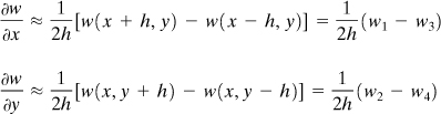
The basic finite difference expressions follow logically from the fundamental rules of calculus. Consider the definition of the first derivative with respect to x of a continuous function y = f(x) (Fig. 7.1):
![]()
Figure 7.1. Finite difference approximation of f(x).
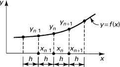
The subscript n denotes any point on the curve. If the increment in the independent variable does not become vanishingly small but instead assumes a finite Δx = h, the preceding expression represents an approximation to the derivative:
![]()
Here Δyn is termed the first difference of y at point xn:
(7.1)
Because the relationship (Fig. 7.1) is expressed in terms of the numerical value of the function at the point in question (n) and a point ahead of it (n + 1), the difference is termed a forward difference. The backward difference at n, denoted ∇yn, is given by
(7.2)
Central differences involve pivot points symmetrically located with respect to xn and often result in more accurate approximations than forward or backward differences. The latter are especially useful where, because of geometrical limitations (as near boundaries), central differences cannot be employed. In terms of symmetrical pivot points, the derivative of y at xn is
(7.3)
The first central difference δy is thus
(7.4)
A procedure similar to that just used will yield the higher-order derivatives.
The second forward difference at xn is expressed in the form
(7.5)
The second backward difference is found in the same way:
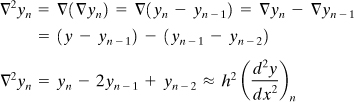
(7.6)
It is a simple matter to verify that the coefficients of the pivot values in the mth forward and backward differences are the same as the coefficients of the binomial expansion (a – b)m. Using this scheme, higher-order forward and backward differences are easily written.
The second central difference at xn is the difference of the first central differences. Therefore,
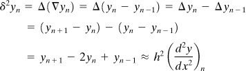
(7.7)
In a like manner, the third and fourth central differences are readily determined:

(7.8)
(7.9)
Examination of Eqs. (7.7) and (7.9) reveals that for even-order derivatives, the coefficients of yn, yn+1 are equal to the coefficients in the binomial expansion (a – b)m.
Unless otherwise specified, we use the term finite differences to refer to central differences.
We now discuss a continuous function w(x, y) of two variables. The partial derivatives may be approximated by the following procedures, similar to those discussed in the previous chapter. For purposes of illustration, consider a rectangular boundary as in Fig. 7.2. By taking Δx = Δy = h, a square mesh or net is formed by the horizontal and vertical lines. The intersection points of these lines are the nodal points. Equation (7.7) yields
(7.10)
(7.11)
Figure 7.2. Rectangular boundary divided into a square mesh.
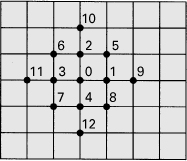
The subscripts x and y applied to the δ’s indicate the coordinate direction appropriate to the difference being formed. The preceding expressions written for the point 0 are
(7.12)
and
(7.13)

Similarly, Eqs. (7.8) and (7.9) lead to expressions for approximating the third- and fourth-order partial derivatives.
7.3 Finite Difference Equations
We are now in a position to transform a differential equation into an algebraic equation. This is accomplished by substituting the appropriate finite difference expressions into the differential equation. At the same time, the boundary conditions must also be converted to finite difference form. The solution of a differential equation thus reduces to the simultaneous solution of a set of linear, algebraic equations, written for every nodal point within the boundary.
Example 7.1. Torsion Bar with Square Cross Section
Analyze the torsion of a bar of square section using finite difference techniques.
Solution
The governing partial differential equation is (see Sec. 6.3)
(7.15)
where Φ may be assigned the value of zero at the boundary. Referring to Fig. 7.2, the finite difference equation about the point 0, corresponding to Eq. (7.15), is
(7.16)
A similar expression is written for every other nodal point within the section. The solution of the problem then requires the determination of those values of Φ that satisfy the system of algebraic equations.
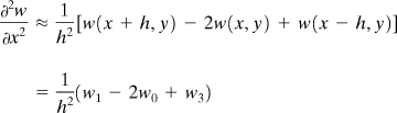
The domain is now divided into a number of small squares, 16 for example. In labeling nodal points, it is important to take into account any conditions of symmetry that may exist. This has been done in Fig. 7.3. Note that Φ = 0 has been substituted at the boundary. Equation (7.16) is now applied to nodal points b, c, and d, resulting in the following set of expressions:

Figure 7.3. Example 7.1. A square cross section of a torsion bar.
Simultaneous solution yields
(a)
The results for points b and d are tabulated in the second column of Table 7.1.
Table 7.1. Values of the Forward Differences for Given Φ’s

To determine the partial derivatives of the stress function, we shall assume a smooth curve containing the values in Eq. (a) to represent the function Φ. Newton’s interpolation formula [Ref. 7.1], used for fitting such a curve, is
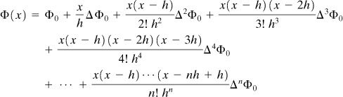
(7.17)
Here the ΔΦ0’s are the forward differences calculated at x = 0 as follows:
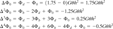
(b)
The differences are also calculated at x = h, x = 2h, and so on, and are listed in Table 7.1. Note that we can readily obtain the values given in Table 7.1 (for the given Φ’s) by starting at node x = 4h: 0 – 1.75 = –1.75, 1.75 – 2.25 = –0.5, –1.75 – (–0.5) = –1.25, and so on.
The maximum shear stress, which occurs at x = 0, is obtained from (∂Φ/∂x)0. Thus, differentiating Eq. (7.17) with respect to x and then setting x = 0, the result is
(c)
Substituting the values in the first row of Table 7.1 into Eq. (c), we obtain
![]()
The exact value, given in Table 6.2 as τmax = 0.678Gθa, differs from this approximation by only 4.7%.
By means of a finer network, we expect to improve the result. For example, selecting h = a/6, six nodal equations are obtained. It can be shown that the maximum stress in this case, 0.661Gθa, is within 2.5% of the exact solution. On the basis of results for h = a/4 and h = a/6, a still better approximation can be found by applying extrapolation techniques.
7.4 Curved Boundaries
It has already been mentioned that one important strength of numerical analysis is its adaptability to irregular geometries. We now turn, therefore, from the straight and parallel boundaries of previous problems to situations involving curved or irregular boundaries. Examination of one segment of such a boundary (Fig. 7.4) reveals that the standard five-point operator, in which all arms are of equal length, is not appropriate because of the unequal lengths of arms bc, bd, be, and bf. When at least one arm is of nonstandard length, the pattern is referred to as an irregular star. One method for constructing irregular star operators is discussed next.
Figure 7.4. Curved boundary and irregular star operator.
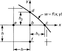
Assume that, in the vicinity of point b, w(x, y) can be approximated by the second-degree polynomial
(7.18)
Referring to Fig. 7.4, this expression leads to approximations of the function w at points c, d, e, and f:
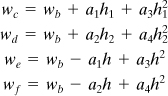
(a)
At nodal point b(x = y = 0), Eq. (7.18) yields
(b)
Combining Eqs. (a) and (b), we have

Introducing this into the Laplace operator, we obtain
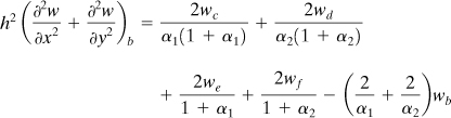
(7.19)
In this expression, α1 = h1/h and α2 = h2/h. It is clear that for irregular stars, 0 ≤ αi ≤ 1(i = 1, 2).
The foregoing result may readily be reduced for one-dimensional problems with irregularly spaced nodal points. For example, in the case of a beam, Eq. (7.19), with reference to Fig. 7.4, simplifies to
(7.20)
where x represents the longitudinal direction. This expression, setting α = α1, may be written
(7.21)
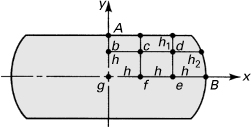
Example 7.2. Elliptical Bar Under Torsion
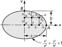
Find the shearing stresses at the points A and B of the torsional member of the elliptical section shown in Fig. 7.5. Let a = 15 mm, b = 10 mm, and h = 5 mm.
Figure 7.5. Example 7.2. Elliptical cross section of a torsion member.
Solution
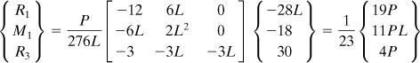
Because of symmetry, only a quarter of the section need be considered. From the equation of the ellipse with the given values of a, b, and h, it is found that h1 = 4.4 mm, h2 = 2.45 mm, h3 = 3 mm. At points b, e, f, and g, the standard finite difference equation (7.18) applies, while at c and d, we use a modified equation found from Eq. (7.15) with reference to Eq. (7.19). We can therefore write six equations presented in the following matrix form:

These equations are solved to yield
![]()
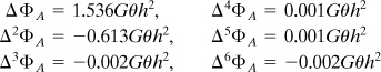
The solution then proceeds as in Example 7.1. The following forward differences at point B are first evaluated:
![]()
Similarly, for point A, we obtain
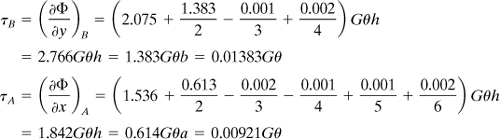
Comment
Note that, according to the exact theory, the maximum stress occurs at y = b and is equal to 1.384Gθb (see Example 6.3), indicating excellent agreement with τB.
7.5 Boundary Conditions
Our concern has thus far been limited to problems in which the boundaries have been assumed free of constraint. Many practical situations involve boundary conditions related to the deformation, force, or moment at one or more points. Application of numerical methods under these circumstances may become more complex.
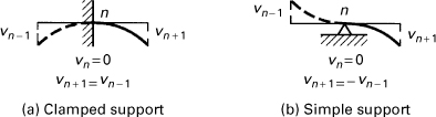
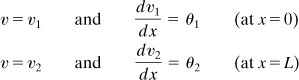
To solve beam deflection problems, the boundary conditions as well as the differential equations must be transformed into central differences. Two types of homogeneous boundary conditions, obtained from v = 0, dv/dx = 0, and v = 0, d2v/dx2 = 0 at a support (n), are depicted in Fig. 7.6a and b, respectively. At a free edge (n), the finite difference boundary conditions are similarly written from d2v/dx2 = 0 and d3v/dx3 = 0 as follows
(a)
Figure 7.6. Boundary conditions in finite differences: (a) clamped or fixed support; (b) simple support.
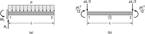
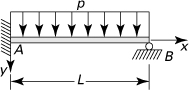
Let us consider the deflection of a nonprismatic cantilever beam with depth varying arbitrarily and of constant width. We shall divide the beam into m segments of length h = L/m and replace the variable loading by a load changing linearly between nodes (Fig. 7.7). The finite difference equations at a nodal point n may now be written as follows. Referring to Eq. (7.7), we find the difference equation corresponding to EI(d2v/dx2) = M to be of the form
(7.22)
Figure 7.7. Finite-difference representation of a nonprismatic cantilever beam with varying load.

The quantities Mn and (IE)n represent the moment and the flexural rigidity, respectively, of the beam at n. In a like manner, the equation EI(d4v/dx4) = p is expressed as
(7.23)
wherein pn is the load intensity at n. Equations identical with the foregoing can be established at each remaining point in the beam. There will be m such expressions; the problem involves the solution of m unknowns, v1, ..., vm.
Applying Eq. (7.4), the slope at any point along the beam is
(7.24)
The following simple examples illustrate the method of solution.
Example 7.3. Displacements of a Simple Beam
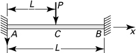
Use a finite difference approach to determine the deflection and the slope at the midspan of the beam shown in Fig. 7.8a.
Figure 7.8. Example 7.3. Simply supported beam with varying load.
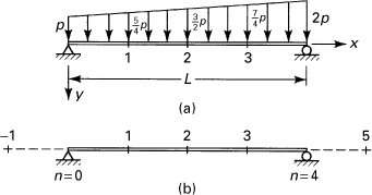
Solution
For simplicity, take h = L/4 (Fig. 7.8b). The boundary conditions v(0) = v(L) = 0 and v″(0) = v″(L) = 0 are replaced by finite difference conditions by setting v(0) = v0, v(L) = v4 and applying Eq. (7.7):
(b)
When Eq. (7.23) is used at points 1, 2, and 3, the following expressions are obtained:
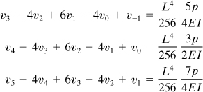
(c)
Simultaneous solution of Eqs. (b) and (c) yields
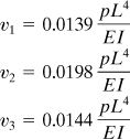
Then, from Eq. (7.24), we obtain
![]()
Note that, by successive integration of EId4v/dx4 = p(x), the result v2 = 0.0185pL4/EI is obtained. Thus, even a coarse segmentation leads to a satisfactory solution in this case.
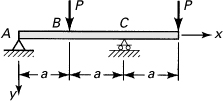
Example 7.4. Reactions of a Continuous Beam
Determine the redundant reaction R for the beam depicted in Fig. 7.9a.
Figure 7.9. Example 7.4. Statically indeterminate beam: (a) load diagram; (b) and (c) moment diagrams.
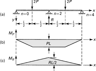
Solution
The bending diagrams associated with the applied loads 2P and the redundant reaction R are given in Figs. 7.9b and c, respectively.
For h = L/2, Eq. (7.22) results in the following expressions at points 1, 2, and 3:

(d)
The number of unknowns in this set of equations is reduced from five to three through application of the conditions of symmetry, v1 = v3, and the support conditions, v0 = v2 = v4 = 0. Solution of Eq. (d) now yields R = 8P/3.
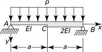
Example 7.5. Stepped Cantilever Beam
Determine the deflection of the free end of the stepped cantilever beam loaded as depicted in Fig. 7.10a. Take h = a/2 (Fig. 7.10b).
Figure 7.10. Example 7.5. Nonprismatic cantilever beam under concentrated loads.
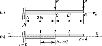
Solution
The boundary conditions v(0) = 0 and v′(0) = 0, referring to Fig. 7.6a, lead to
(e)
The moments are M0 = 3Pa, M1 = 2Pa, M2 = Pa, and M3 = Pa/2. Applying Eq. (7.22) at nodes 0, 1, 2, and 3, we obtain
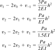
(f)
Observe that at point 2, the average flexural rigidity is used. Solving Eqs. (e) and (f) gives v1 = 3C/4, v2 = 5C/2, v3 = 59C/12, and v4 = 47C/6, in which C = (Pa/EI)h2. Therefore, after setting h = a/2, we have
![]()
The foregoing deflection is about 2.2% larger than the exact value.
Part B—Finite Element Method
7.6 Fundamentals
Structural analysis involves the determination of the forces and deflections within a structure or its members. The earliest demands for structural analysis led to a host of so-called classical methods. The specialization of the classical methods was replaced by generalities of the modern matrix methods. The presentation of this chapter is limited to the most widely used of these techniques: the finite element stiffness or displacement method. Unless otherwise specified, we shall refer to it as the finite element method (FEM). The finite element analysis (FEA) is a numerical approach and well suited to digital computers. The method relies on the formulations of a simultaneous set of algebraic equations relating forces to corresponding displacements at discrete preselected points (called nodes) on the structure. These governing algebraic equations, also called the force–displacement relations, are expressed in matrix notations.
The powerful finite element method had its beginnings in the 1980s, and with the advent of high-speed, large-storage-capacity digital computers, it has gained great prominence throughout the industries in the solution of practical analysis and design problems of high complexity. The FEA offers many advantages. The structural geometry can be readily described, and combined load conditions can be easily handled. It offers the ability to treat discontinuities, to handle composite and anisotropic materials, to handle unlimited numbers and kinds of boundary conditions, to handle dynamic and thermal loadings, and to treat nonlinear structural problems. It also has the capacity for complete automation. The literature related to the FEA is extensive. See, for example, Refs. 7.2 through 7.20. Numerous commercial FEA software programs are available, as described in Section 7.16, including some directed at the learning process.
The basic concept of the finite element approach is that the real structure can be divided or discretized by a finite number of elements, connected not only at their nodes but along the interelement boundaries as well. Triangular, rectangular, tetrahedron, quadrilateral, or hexagonal forms of elements are often employed in the finite element method. The types of elements that are commonly used in structural idealization are the truss, beam, two-dimensional elements, shell and plate bending, and three-dimensional elements. Figure 7.11a depicts how a multistory hotel building is modeled using bar, beam, column, and plate elements, which can be employed for static, free vibration, earthquake response, and wind response analysis [Ref. 7.2]. A model of a nozzle in a thin-walled cylinder, created using triangular shell elements, is shown in Fig. 7.11b. Similarly, large structural systems, such as air-crafts or ships, are usually analyzed by dividing the structure into smaller units or substructures (e.g., wing of an airplane). When the stiffness of each unit has been determined, the analysis of the system follows the familiar procedure of matrix methods used in structural mechanics.
Figure 7.11. Finite element models of two structures: (a) Multistory building; (b) pipe connection (Ref. 7.8).

The network of elements and nodes that discretize the region is called a mesh. The density of a mesh increases as more elements are placed within a given region. Mesh refinement is when the mesh is modified in an analysis of a model to give improved solutions. Mesh density is increased in areas of high stress concentrations and when geometric transition zones are meshed smoothly (Fig. 7.11b). Usually, the FEA results converge toward the exact results as the mesh is continuously refined. To discuss adequately the subject of the FEA would require a far more lengthy presentation than could be justified here. However, the subject is sufficiently important that engineers concerned with the analysis and design of members should have at least an understanding of the FEA. The fundamentals presented can clearly show the potential of the FEA as well as its complexities. It can be covered as an option, used as a “teaser” for a student’s advance study of the topic, or used as a professional reference.
7.7 The Bar Element
A bar element, also called a truss bar element or axial element, represents the simplest form of structural finite element. An element of this type of length L, modulus of elasticity E, and cross-sectional area A, is denoted by e (Fig. 7.12). The two ends or joints or nodes are numbered 1 and 2, respectively. A set of two equations in matrix form are required to relate the nodal forces (![]() and
and ![]() ) to the nodal displacements (
) to the nodal displacements (![]() and
and ![]() ).
).
Figure 7.12. The one-dimensional axial element (e).

Equilibrium Method
The direct equilibrium approach is simple and physically clear, but it is practically well suited only for truss, beam, and frame elements. The equilibrium of the x-directed forces requires that ![]() (Fig. 7.12). In terms of the spring rate AE/L of the element, we have
(Fig. 7.12). In terms of the spring rate AE/L of the element, we have
![]()
This may be written in matrix form,
(7.25a)
or symbolically,
(7.25b)
The quantity ![]() is called the element stiffness matrix with dimensions of force per unit displacement. It relates the nodal displacements
is called the element stiffness matrix with dimensions of force per unit displacement. It relates the nodal displacements ![]() to the nodal forces
to the nodal forces ![]() on the element.
on the element.
Energy Method
The energy approach is more general, easier to apply, and more powerful than the direct method discussed in the foregoing, particularly for complex kinds of finite elements (see Ref. 7.2). Using this technique, it is necessary to first define a displacement function for the element (Fig. 7.12):
(7.26)
where a1 and a2 are constants. Clearly, Eq. (7.26) represents a continuous linear displacement variation along the x axis of the element that corresponds to that of engineering formulation for a bar under axial loading. The axial displacements of joints 1 (at x = 0) and 2 (at ![]() ), respectively, are
), respectively, are
![]()
Solving, we have ![]() and
and ![]() . Carrying these results into Eq. (7.26), we obtain
. Carrying these results into Eq. (7.26), we obtain
(7.27)
Using Eq. (7.27), we write
(7.28)
Thus, the axial force in the element is
(7.29)
Substituting Eq. (7.29) into Eq. (2.58), the strain energy in the element may be expressed as follows
(7.30)
Then, Castigliano’s first theorem, Eq. (10.22), gives
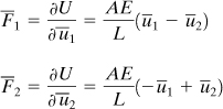
The matrix form of these equations is the same as that given by Eqs. (7.25).
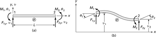
7.8 Arbitrarily Oriented Bar Element
The global stiffness matrix for an element oriented arbitrarily in a two-dimensional plane is developed in this section. The local coordinates are chosen to conveniently represent the individual element. On the other hand, the reference or global coordinates are chosen to be convenient for the entire structure (Fig. 7.13). The local and global coordinates systems for an axial element are designated by ![]() ,
, ![]() and x, y, respectively.
and x, y, respectively.
Figure 7.13. Global coordinates (x, y) for plane truss and local coordinates (![]() ,
, ![]() ) for a bar element 1-2.
) for a bar element 1-2.

Coordinate Transformation
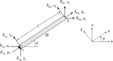
A typical axial element e lying along the x axis, which is oriented at an angle θ, measured counterclockwise from the reference axis x, is shown in Fig. 7.14. In the local coordinate system, each joint has an axial force ![]() , a transverse force
, a transverse force ![]() , an axial displacement
, an axial displacement ![]() , and a transverse displacement
, and a transverse displacement ![]() . Referring to the figure, Eq. (7.25a) may be expanded as follows:
. Referring to the figure, Eq. (7.25a) may be expanded as follows:
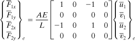
(7.31a)
Figure 7.14. Local (![]() ,
, ![]() ) and global (x, y) coordinates for a two-dimensional bar element (e).
) and global (x, y) coordinates for a two-dimensional bar element (e).
or concisely,
(7.31b)
The quantities ![]() and
and ![]() are the stiffness and nodal displacement matrices, respectively, in the local coordinate system.
are the stiffness and nodal displacement matrices, respectively, in the local coordinate system.
Force Transformation
It is seen from Fig. 7.14 that the two local and global forces at joint 1 may be related by the following expressions:
![]()
Similar equations apply at joint 2. For brevity, let
(a)
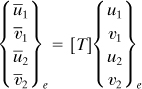
Hence, the local and global forces are related in the matrix form as
(7.32a)
or symbolically,
(7.32b)
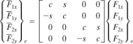
In Eq. (7.32b), [T] represents the coordinate transformation matrix:
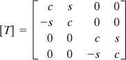
(7.33)
The {F}e is the global nodal force matrix

(7.34)
We note that the coordinate transformation matrix satisfies the following conditions of orthogonality: c2 + s2 = 1, (–s)2 + c2 = 1, and (–s)(c) + (c)(s) = 0. Thus, the [T] is an orthogonal matrix.
Displacement Transformation
Inasmuch as the displacement transforms in an identical way as forces, we can write
(7.35a)
The concise form of this is
(7.35b)
where {δ} is the global nodal displacements. Carrying Eqs. (7.35b) and (7.32b) into (7.31b) results in
![]()
from which
![]()
The inverse of the orthogonal matrix [T] is the same as its transpose: [T] = [T]T. Here the superscript T denotes the transpose. It is recalled that the transpose of a matrix is found by interchanging the rows and columns of the matrix.
Governing Equations
The global force–displacement relations or the governing equations for an element e are thus expressed in the form
(7.36)
where
(7.37)
The global stiffness matrix for the element, substituting Eq. (7.33) and [k] from Eq. (7.31a) into Eq. (7.37), may be written as
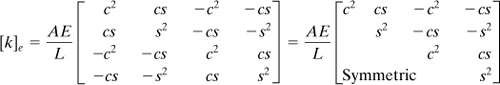
(7.38)
The foregoing indicates that the element stiffness matrix depends on its dimensions, orientation, and material property.
7.9 Axial Force Equation
Reconsider the general case of a truss element 1–2 oriented arbitrarily in a two-dimensional plane, shown in Fig. 7.14. We multiply the third and fourth expressions in Eq. (7.36) to obtain the global forces at node 2 as
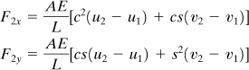
The axial tensile force in the element with nodes 1 and 2, designated by F12, is then
F12 = F2xc + F2ys
in which cosθ = c and sinθ = s. It is seen that this force is equivalent to the nodal force ![]() or
or ![]() associated with local coordinates
associated with local coordinates ![]() 1 and
1 and ![]() 2.
2.
Combining the preceding relationships leads to
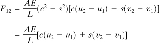
(a)
or
F12 = (spring rate)(total axial elongation)
Here, the quantities (u2 – u1) and (v2 – v1) are, respectively, the horizontal and vertical components of the axial elongation. Equation (a) may be expressed in the matrix form
![]()
The axial force in the bar element with nodes ij is thus
(7.39)
A positive (negative) value obtained for Fij indicates that the element is in tension (compression). The axial stress, in element of cross-sectional area A, then is σij = Qij/A.
Example 7.6. Properties of a Truss Bar Element
The element 1–2 of the steel truss shown in Fig. 7.13 with a length L, cross-sectional area A, and modulus of elasticity E, is oriented at angle θ counterclockwise from the x axis. Given:
![]()
Calculate (a) the global stiffness matrix for the element; (b) the local displacements ![]() ,
, ![]() ,
, ![]() , and
, and ![]() of the element; (c) the axial stress in the element.
of the element; (c) the axial stress in the element.
Solution
The free-body diagram of the element 1–2 is shown in Fig. 7.15. The spring rate of the element is
![]()
Figure 7.15. Example 7.6. An axially loaded bar.

and
![]()
a. Element Stiffness Matrix. Applying Eq. (7.38),
or
b. Element Displacements. Equations (7.35b), ![]() , results in
, results in
c. Axial Force. Substituting the given numerical values into Eq. (7.39) with i = 1 and j = 2, we find
![]()
It follows that axial stress in the element is equal to σ1 = F1/A = –244 MPa.
Comment
The negative sign indicates a compression.
7.10 Force-Displacement Relations for a Truss
We now develop the finite element method by considering a plane truss. A truss is a structure composed of differently oriented straight bars connected at their joints (or nodes) by means of pins, such as shown Fig. 7.13. It is easier to understand the basic procedures of treatment by referring to this simple system. The general derivation of the FEM will be discussed in Section 7.13. To derive truss equations, the global element relations for the axial element given by Eq. (7.36) will be assembled. This gives the following force-displacement relations for the entire truss or the system equations:
(7.40)
The global nodal matrix {F} and the global stiffness matrix [K] are expressed as
(7.41)
and
(7.42)
Here the quantity e designates an element and n is the number of elements comprising the truss. Observe that [K] relates the global nodal force {F} to the global displacement {δ} for the entire truss.
The Assembly Process
The element stiffness matrices [k]e in Eq. (7.38) must be properly added together or superimposed. To perform direct addition, a convenient method is to label the columns and rows of each element stiffness matrix in accordance to the displacement components related with it. The truss stiffness matrix [K] is then found simply by summing terms from the individual element stiffness matrix into their corresponding locations in [K]. Alternatively, expand the [k]e for each element to the order of the truss stiffness matrix by adding rows and columns of zeros. We shall employ this process of assemblage of the element stiffness matrices. It is obvious that, for the problems involving a large number of elements, to implement the assembly of the [K] requires a digital computer.
The use of the fundamental equations developed are illustrated in the solution of the following sample numerical problems.
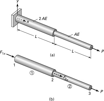
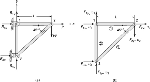
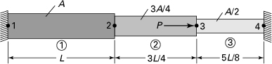
Example 7.7. Stepped Axially Loaded Bar
A bar consists of two prismatic parts, fixed at the left end, and supports a load P at the right end, as illustrated in Fig. 7.16a. Determine the nodal displacements and nodal forces in the bar.
Figure 7.16. Example 7.7. (a) A stepped bar under an axial load; (b) two-element model.
Solution
In this case, the global coordinates (x, y) coincide with local (![]() ,
, ![]() ) coordinates. The bar is discretized into elements with nodes 1, 2, and 3 (Fig. 7.16b). The axial rigidities of the elements 1 and 2 are 2AE and AE, respectively. Therefore, (AE/L)1 = 2AE/L and (AE/L)2 = AE/L.
) coordinates. The bar is discretized into elements with nodes 1, 2, and 3 (Fig. 7.16b). The axial rigidities of the elements 1 and 2 are 2AE and AE, respectively. Therefore, (AE/L)1 = 2AE/L and (AE/L)2 = AE/L.
Element Stiffness Matrices. Through the use of Eq. (7.25), the stiffness for the elements 1 and 2 is expressed as

It is seen that the column and row of each stiffness matrix are labeled according to the nodal displacements associated with them. There are three displacement components (u1, u2, u3), and hence the order of the system matrix must be 3 × 3. In terms of the bar displacements, we write
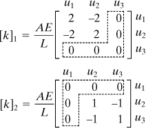
In the foregoing matrices, the last row and first column of zeros are added, respectively (boxed in by the dashed lines).
Stiffness Matrix System. The superposition of the terms of each stiffness matrix leads to
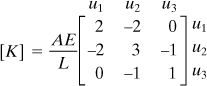
Force–Displacement Relations. Equations (7.40) are expressed as

(a)
The displacement and force boundary conditions are u1 = 0, F2x = 0, and F3x = P. Then, Eqs. (a), referring to Fig. 7.16b,
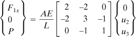
Displacements. To determine u2 and u3, only the part of this equations is considered:
![]()
Solution of this equation equals
![]()
Comment
With the displacements available, the axial force and stress in the element 1 (or 2) can readily be found as described in Example 7.6.
Nodal Forces. Equations (a) gives

Comment
The results indicate that the reaction F1x = –P is equal in magnitude but opposite in direction to the applied force at node 3, F3x = P. Also, F2x = 0 shows that no force is applied at node 2. Equilibrium of the bar assembly is thus satisfied.
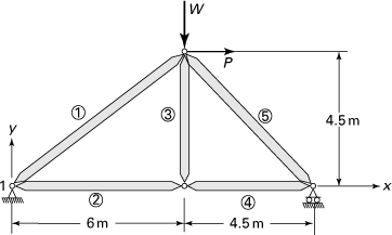
Example 7.8. Analysis of a Three-Bar Truss
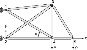
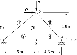
A steel plane truss in which all members have the same axial rigidity AE supports a horizontal force P and a load W acting at joint 2, as shown in Fig. 7.17a. Find the nodal displacements, reactions, and stresses in each member. Given:
![]()
Figure 7.17. Example 7.8. (a) Basic plane truss; (b) finite element model.
Solution
The reactions are marked and the nodes numbered arbitrarily for elements in Fig. 7.17a.
Input Data. At each node there are two displacements and two nodal force components (Fig. 7.17b). It is recalled that θ is measured counterclockwise from the positive x axis to each element (Table 7.2).
Table 7.2. Data for the Truss of Fig. 7.17

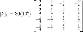
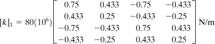
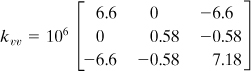
Element Stiffness Matrix. Applying Eq. (7.38) and Table 7.2, we have for the bars 1, 2, and 3, respectively:

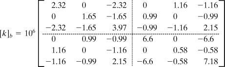
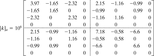
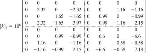
In the preceding, the column and row of each stiffness matrix are labeled according to the nodal displacements associated with them. It is seen that displacements u3 and v3 are not involved in element 1; the u2 and v2 are not involved in element 2; the u1 and v1 are not involved in element 3. Thus, prior to adding [k]1, [k]2, and [k]3 to obtain the system matrix, two rows and columns of zeros must be added to each of the element matrices to account for the absence of these displacements. It follows that, using a common factor 107, element stiffness matrices take the forms
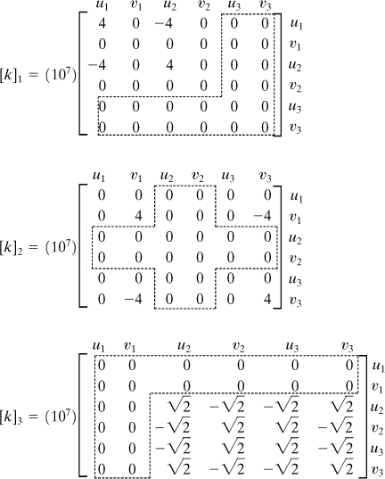
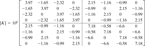
System Stiffness Matrix. There are a total of six components of displacement for the truss before boundary constraints are imposed. Hence, the order of the truss stiffness matrix must be 6 × 6. After adding the terms from each element stiffness matrix into their corresponding locations in [K], we readily determine the global stiffness matrix for the truss as
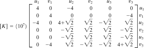
(b)
System Force–Displacement Relationship. With reference to Fig. 7.11, the boundary conditions are u1 = 0, v1= 0, u3 = 0. In addition, we have F3y = 0. Then, Eq. (7.40) becomes
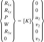
(c)
where [K] is given by Eq. (b).
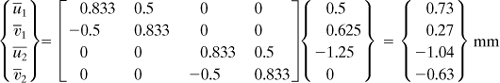
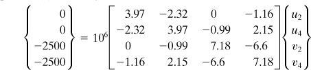
Displacements. To find u2, v2, and v3, only part of Eq. (c) associated with these displacements is considered. In so doing, we have
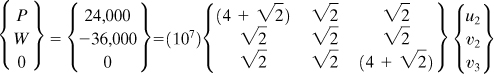
(d)
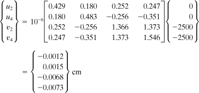
Inversion of the preceding gives

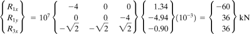
Reactions. Carrying the foregoing values of u2, v2, and v3 into Eq. (c) results in the reactional forces as
The results may be verified by applying the equilibrium equations to the free-body diagram of the entire truss, Fig. 7.17a.
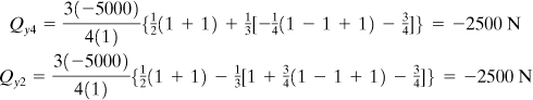
Axial Forces in Elements. From Eqs. (7.39) and (d) and Table 7.2, we obtain
![]()

Stresses in Elements. By dividing the preceding element forces by the cross-sectional area of each bar, we obtain

The negative sign indicates a compressive stress.
Comment
The results indicate that member axial stresses are well below the yield strength for the material considered. Observe that the FEA permits the calculation of displacements, forces, and stresses in the truss with unprecedented ease and precision. It is evident, however, that the FEA, even in the simplest cases, requires considerable algebra. For any significant problem, the electronic digital computer must be used.
7.11 Beam Element
This section provides only a brief discussion of the development of a stiffness matrix for beam elements. Let us consider an initially straight beam element of uniform flexural rigidity EI and length L (Fig. 7.18a). The element has a transverse deflection v and a slope θ = dv/dx at each end or node. Corresponding to these displacements, a transverse shear force F and a bending moment M act at each node. The deflected configuration of the beam element is depicted in Fig. 7.18b.
Figure 7.18. The beam element with nodal forces and displacements: (a) before deformation; (b) after deformation.
The linearly elastic behavior of a beam element is governed by Eq. (5.32) as d4v/dx4 = 0. Observe that the right-hand side of this equation is zero because in the formulation of the stiffness matrix equations, we assume no loading between nodes. In the elements where there is a distributed load (see Example 7.9) or a concentrated load between the nodes, the equivalent nodal load components listed in Table D.5 of Appendix D are employed. Note that the equivalent nodal loads correspond to the (oppositely directed) reactions provided by a beam subject to the distributed or concentrated loading under fixed-fixed boundary conditions. For further details, see Ref. 7.6.
The solution of the governing equation is assumed, a cubic polynomial function of x, as follows
(a)
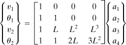
It is seen that the number of terms in the preceding expression is the same as the number of nodal displacements of the element. Equation (a) satisfies the basic beam equation, the conditions of displacement, and the continuity of interelement nodes. The coefficients a1, a2, a3, and a4 are obtained from the conditions at both nodes:
(b)
Introducing Eq. (a) into (b) leads to
The inverse of these equations is

Substituting the foregoing expressions into Eq. (a) yields the displacement function in the form
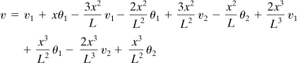
(7.43)
The bending moment M and shear force V in an elastic beam with cross section that is symmetrical about the plane of loading are related to the displacement function by Eqs. (5.32). Therefore,
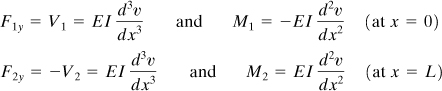
(7.44)
in which the minus signs in the second and third expressions are due to opposite to the sign conventions adopted for V and M in Figs. 5.7b and 7.18.
It can be verified [Ref. 7.2] that inserting Eq. (7.43) into Eqs. (7.44) gives the nodal force (moment)–deflection (slope) relations in the matrix form as
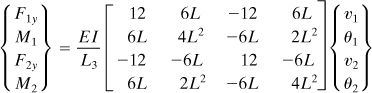
(7.45a)
or symbolically,
(7.45b)
in which the matrix [k]e represents the force and moment components. Likewise, {δ}e represents both deflections and slopes. The element stiffness matrix lying along a coordinate x is then
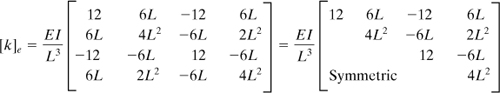
(7.46)
With development of the stiffness matrix, formulation and solution of problems involving beam elements proceeds like that of bar elements, as demonstrated in the examples to follow.
Example 7.9. Displacements of a Uniformly Loaded Cantilever Beam
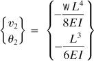
A cantilever beam of length L and flexural rigidity EI carries a uniformly distributed load of intensity p, as illustrated in Fig. 7.19a. Find the vertical deflection and rotation at the free end.
Figure 7.19. Example 7.9. (a) Beam with distributed load; (b) the equivalent nodal forces.
Solution
Only one finite element to represent the entire beam is used. The distributed load is replaced by the equivalent forces and moments, as shown in Fig. 7.19b (see case 3 in Table D.4). The boundary conditions are given by
![]()
![]()
Then, the force–displacement relations, Eqs. (7.45a), simplifies to

Solving for the displacements,

Subsequent to the multiplication, we obtain
Comment
The minus sign indicates a downward deflection and a clockwise rotation at the right end, node 2.
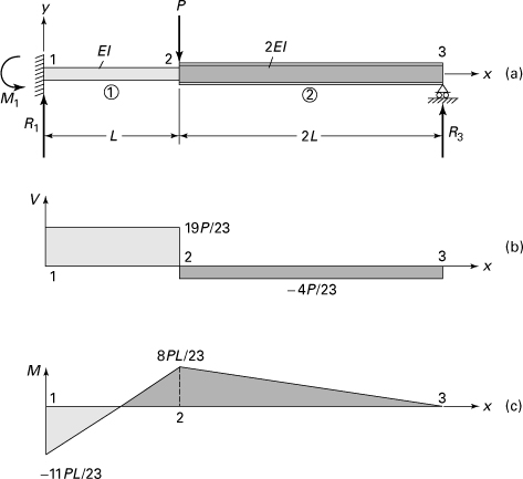
Example 7.10. Analysis of a Statically Indeterminate Stepped Beam
A propped cantilever beam of flexural rigidity EI and 2EI for the parts 1–2 and 2–3, respectively, supports a concentrated load P at point 2 (Fig. 7.20a). Calculate (a) the nodal displacements; (b) the nodal forces and moments.
Figure 7.20. Example 7.10. (a) Stepped beam with a load; (b) shear diagram; (c) bending moment diagram.
Solution
The beam is discretized into elements 1 and 2 with nodes 1, 2, and 3, as illustrated in Fig. 7.20a. There are a total of six displacement components for the beam before the boundary conditions are applied. The order of the system stiffness matrix must therefore be 6 × 6.
Applying Eq. (7.46), the stiffness matrix for the element 1, with (EI/L3)1 = EI/L3 and L1 = L, may be written as

(c)
Likewise, with (EI/L3)2 = EI/4L3 and L2 = 2L, for element 2, after rearrangement:
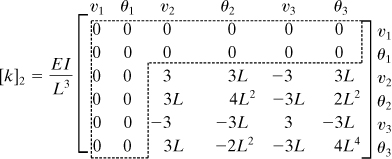
Note that, in the preceding, the nodal displacements are shown to indicate the associativity of the rows and columns of the member stiffness matrices. Hence, rows and columns of zeros are added (boxed in by the dashed lines).
a. The system stiffness matrix of the beam can now be superimposed [K] = [k]1 + [k]2. The beam governing equations, with F2y = –P (Fig. 7.20b), are therefore
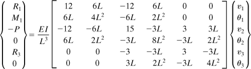
(7.47)
The boundary conditions are v1 = 0, θ1 = 0, and v3 = 0. After multiplying these equations with the corresponding unknown displacements, we obtain
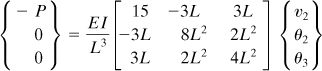
(d)
and
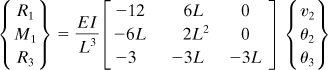
(e)
Solving Eqs. (d), we find deflection and slopes as follows:
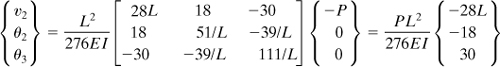
The minus sign means a downward deflection at node 2 and clockwise rotation of left end 1; the positive sign means a counterclockwise rotation at right end 3 (Fig. 7.20), as appreciated intuitively.
b. Substituting the displacements found into Eq. (e), after multiplying and simplifying, nodal forces and moments are
Comment
Usually, it is necessary to obtain the nodal forces and moments associated with each element to analyze the whole structure. For the case under consideration, it may readily be seen from a free-body diagram of element 2 that M2 = R3 (2L) = 8PL/23. So, we have the shear and moment diagrams for the beam, as shown in Figs. 7.20b and c, respectively.
7.12 Properties of Two-Dimensional Elements
Now we define a number of basic quantities relevant to an individual finite element of an isotropic elastic body. In the interest of simple presentation, in this section the relationships are written only for the two-dimensional case. The general formulation of the finite element method applicable to any structure is presented in the next section. Solutions of plane stress and plane strain problems are illustrated in detail in Section 7.14. The analyses of axisymmetric structures and thin plates employing the finite element are given in Chapters 8 and 13, respectively.
To begin with, the relatively thin, continuous body shown in Fig. 7.21a is replaced or discretized by an assembly of finite elements (triangles, for example) indicated by the dashed lines (Fig. 7.21b). These elements are connected not only at their corners or nodes but along the interelement boundaries as well. The basic unknowns are the nodal displacements.
Figure 7.21. Plane stress region (a) before and (b) after division into finite elements.

Displacement Matrix
The nodal displacements are related to the internal displacements throughout the entire element by means of a displacement function. Consider the typical element e in Fig. 7.21b, shown isolated in Fig. 7.22a. Designating the nodes i, j, and m, the element nodal displacement matrix is
(7.48a)
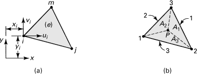
Figure 7.22. Triangular finite element.
or, for convenience, expressed in terms of submatrices δu and δv,
(7.48b)
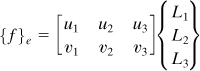
where the braces indicate a column matrix. The displacement function defining the displacement at any point within the element, {f}e, is given by
(7.49)
which may also be expressed as
(7.50)
where the matrix [N] is a function of position, to be obtained later for a specific element. It is desirable that a displacement function {f}e be selected such that the true displacement field will be represented as closely as possible. The approximation should result in a finite element solution that converges to the exact solution as the element size is progressively decreased.
Strain, Stress, and Elasticity Matrices
The strain, and hence the stress, are defined uniquely in terms of displacement functions (see Chap. 2). The strain matrix is of the form
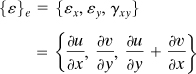
(7.51a)
or
(7.51b)
where [B] is also yet to be defined.
Similarly, the state of stress throughout the element is, from Hooke’s law,

(a)
Succinctly,
(7.52)
where [D], an elasticity matrix, contains material properties. If the element is subjected to thermal or initial strain, the stress matrix becomes
(7.53)
The thermal strain matrix, for the case of plane stress, is given by {ε0} = {αT, αT, 0} (Sec. 3.8). Comparing Eqs. (a) and (7.52), it is clear that
(7.54)
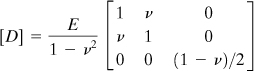
In general, the elasticity matrix may be represented in the form
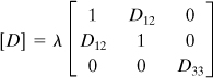
(7.55)
It is recalled from Section 3.5 that two-dimensional problems are of two classes: plane stress and plane strain. The constants λ, D12, and D33 for a two-dimensional problem are given in Table 7.3.
Table 7.3. Elastic Constants for Two-Dimensional Problems
7.13 General Formulation of the Finite Element Method
A convenient method for executing the finite element procedure relies on the minimization of the total potential energy of the system, expressed in terms of displacement functions. Consider again in this regard an elastic body (Fig. 7.21). The principle of potential energy, from Eq. (10.21), is expressed for the entire body as follows:
(7.56)
Note that variation notation δ has been replaced by Δ to avoid confusing it with nodal displacement. In Eq. (7.56),
Through the use of Eq. (7.49), Eq. (7.56) may be expressed in the following matrix form:
(a)
where superscript T denotes the transpose of a matrix. Now, using Eqs. (7.50), (7.51), and (7.53), Eq. (a) becomes
(b)
The element stiffness matrix [k]e and element nodal force matrix {Q}e (due to body force, initial strain, and surface traction) are
(7.57)
(7.58)
It is clear that the variations in {δ}e are independent and arbitrary, and from Eq. (b) we may therefore write
(7.59)
We next derive the governing equations appropriate to the entire continuous body. The assembled form of Eq. (b) is
(c)
This expression must be satisfied for arbitrary variations of all nodal displacements {Δδ}. This leads to the following equations of equilibrium for nodal forces for the entire structure, the system equations:
(7.60)
where
(7.61)
It is noted that structural matrix [K] and the total or equivalent nodal force matrix {Q} are found by proper superposition of all element stiffness and nodal force matrices, respectively, as discussed in Section 7.10 for trusses.
Outline of General Finite Element Analysis
We can now summarize the general procedure for solving a problem by application of the finite element method as follows:
1. Calculate [k]e from Eq. (7.57) in terms of the given element properties. Generate [K] = Σ[k]e.
2. Calculate {Q}e from Eq. (7.58) in terms of the applied loading. Generate {Q} = Σ{Q}e.
3. Calculate the nodal displacements from Eq. (7.60) by satisfying the boundary conditions: {δ} = [K]–1{Q}.
4. Calculate the element strain using Eq. (7.51): {ε}e = [B]{δ}e.
5. Calculate the element stress using Eq. (7.53): {σ}e = [D]({ε} – {ε0})e.
A simple block diagram of finite element analysis is shown in Fig. 7.23.
Figure 7.23. The finite element analysis block diagram [Ref. 7.8].

When the stress found is uniform throughout each element, this result is usually interpreted two ways: the stress obtained for an element is assigned to its centroid; if the material properties of the elements connected at a node are the same, the average of the stresses in the elements is assigned to the common node.
The foregoing outline will be better understood when applied to a triangular element in the next section. Formulation of the properties of a simple one-dimensional element, using relations developed in this section, is illustrated in the following example.
Example 7.11. Deflection of a Bar under Combined Loading
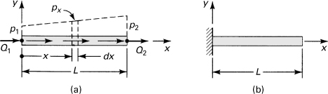
A bar element of constant cross-sectional area A, length L, and modulus of elasticity E is subjected to a distributed load px per unit length and a uniform temperature change T (Fig. 7.24a). Determine (a) the stiffness matrix, (b) the total nodal force matrix, and (c) the deflection of the right end u2 for fixed left end and px = 0 (Fig. 7.24b).
Figure 7.24. Example 7.11. (a) Bar element subjected to an axial load px and uniform temperature change T; (b) fixed end bar.
Solution
a. As before (see Sec. 7.7), we shall assume that the displacement u at any point within the element varies linearly with x:
(d)
wherein a1 and a2 are constants. The axial displacements of nodes 1 and 2 are u1 = a1 and u2 = a1 + a2L from which a2 = – (u1 – u2)/L. Substituting this into Eq. (d),
(e)
Applying Eq. (7.51a), the strain in the element is
![]()
(f)
For a one-dimensional element, we have D = E, and the stress from Eq. (7.52) equals
![]()
The element stiffness matrix is obtained upon introduction of [B] from Eq. (f) into Eq. (7.57):
(7.62)
b. Referring to Fig. 7.24a,
(7.63)
where p1 and p2 are the intensities of the load per unit length at nodes 1 and 2, respectively. Substitution of [N] from Eq. (e) together with Eq. (7.63) into Eq. (7.58) yields
![]()
The distributed load effects are obtained by integrating the preceding equations:
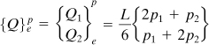
(g)
The strain due to the temperature change is ε0 = αT, where α is the coefficient of thermal expansion. Inserting [B] from Eq. (f) into Eq. (7.58),
![]()
The thermal strain effects are then
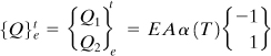
(h)
The total element nodal matrix is obtained by adding Eqs. (g) and (h):
(7.64)
c. The nodal force-displacement relations (7.60) now take the form
![]()
from which the elongation of the bar equals u2 = α(T)L, a predictable result.
7.14 Triangular Finite Element
Because of the relative ease with which the region within an arbitrary boundary can be approximated, the triangle is used extensively in finite element assemblies. Before deriving the properties of the triangular element, we describe area or triangular coordinates, which are very useful for the simplification of the displacement functions.
In this section, we derive the basic constant strain triangular (CST) plane stress and strain element. Note that there are a variety of two-dimensional finite element types that lead to better solutions. Examples are linear strain triangular (LST) elements, triangular elements having additional side and interior nodes, rectangular elements with corner nodes, and rectangular elements having additional side nodes [Refs. 7.4, 7.6]. The LST element has six nodes: the usual corner nodes plus three additional nodes located at the midpoints of the sides. The procedures for the development of the LST element equations follow the identical steps as that of the CST element.
Consider the triangular finite element 1 2 3 (where i = 1, j = 2, and m = 3) shown in Fig. 7.22b, in which the counterclockwise numbering convention of nodes and sides is indicated. A point P located within the element, by connection with the corners of the element, forms three subareas denoted A1, A2, and A3. The ratios of these areas to the total area A of the triangle locate P and represent the area coordinates:
(7.65)
(7.66)
and consequently only two of the three coordinates are independent. A useful property of area coordinates is observed through reference to Fig. 7.22b and Eq. (7.65):
![]()
and
The area A of the triangle may be expressed in terms of the coordinates of two sides, for example, 2 and 3:
![]()
or
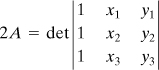
(7.67a)
Here i, j, and k are the unit vectors in the x, y, and z directions, respectively. Two additional expressions are similarly found. In general, we have
(7.67b)
where
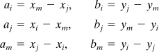
(7.68)
Note that aj, am, bj, and bm can be found from definitions of ai and bi with the permutation of the subscripts in the order ijmijm, and so on.
Similar equations are derivable for subareas A1, A2, and A3. The resulting expressions, together with Eq. (7.65), lead to the following relationship between area and Cartesian coordinates:
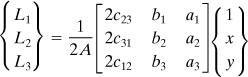
(7.69)
where
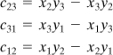
(7.70)
Note again that, given any of these expressions for cij, the others may be obtained by permutation of the subscripts.
Now we explore the properties of an ordinary triangular element of a continuous body in a state of plane stress or plane strain (Fig. 7.22). The nodal displacements are
(a)
The displacement throughout the element is provided by
(7.71)
Matrices [N] and [B] of Eqs. (7.50) and (7.51b) are next evaluated, beginning with
(b)
(c)
We observe that Eqs. (7.71) and (b) are equal, provided that
(7.72)
The strain matrix is obtained by substituting Eqs. (7.71) and (7.69) into Eq. (7.51a):
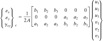
(d)
Here A, ai, and bi are defined by Eqs. (7.67) and (7.68). The strain (stress) is observed to be constant throughout, and the element of Fig. 7.22 is thus referred to as a constant strain triangle. Comparing Eqs. (c) and (d), we have
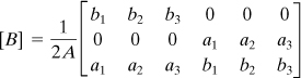
(7.73)
The stiffness of the element can now be obtained through the use of Eq. (7.57):
(e)

(7.74)
where [D] is given by Eq. (7.54) for plane stress. Assembling Eq. (e) together with Eqs. (7.73) and (7.74) and expanding, the stiffness matrix is expressed in the following partitioned form of order 6 × 6:
(7.75)
where the submatrices are

(7.76)
Element Nodal Forces
Finally, we consider the determination of the element nodal force matrices. The nodal force owing to a constant body force per unit volume is, from Eqs. (7.58) and (7.72),
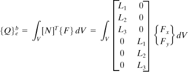
(f)
For an element of constant thickness, this expression is readily integrated to yield*
(7.77)
The nodal forces associated with the weight of an element are observed to be equally distributed at the nodes.
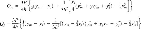
The element nodal forces attributable to applied external loading may be determined either by evaluating the static resultants or by application of Eq. (7.58). Nodal force expressions for arbitrary nodes j and m are given next for a number of common cases (Prob. 7.40).
Linear load, p(y) per unit area, Fig. 7.25a:
(7.78a)
Figure 7.25. Nodal forces due to (a) linearly distributed load and (b) shear load.

where t is the thickness of the element.
Uniform load is a special case of the preceding with pj = pm = p:
(7.78b)
End shear load, P, the resultant of a parabolic shear stress distribution defined by Eq. (3.24) (see Fig. 7.25b):
(7.79)
Equation (7.75), together with those expressions given for the nodal forces, characterizes the constant strain element. These are substituted into Eq. (7.61) and subsequently into Eq. (7.60) in order to evaluate the nodal displacements by satisfying the boundary conditions.
The basic procedure employed in the finite element method is illustrated in the following simple problems.
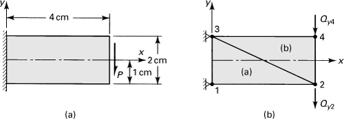
Example 7.12. Nodal Forces of a Plate Segment under Combined Loading
The element e shown in Fig. 7.26 represents a segment of a thin elastic plate having side 2–3 adjacent to its boundary. The plate is subjected to several loads as well as a uniform temperature rise of 50°C. Determine (a) the stiffness matrix and (b) the equivalent (or total) nodal force matrix for the element if a pressure of p = 14 MPa acts on side 2–3. Let t = 0.3 cm, E = 200 GPa, v = 0.3, specific weight γ = 77 kN/m3, and α = 12 × 10–6/°C.
Figure 7.26. Example 7.12. A triangular plate.
Solution
The origin of the coordinates is located at midlength of side 1–3, for convenience. However, it may be placed at any point in the x, y plane. Applying Eq. (7.74), we have (in N/cm3)
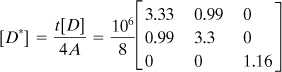
(g)
a. Stiffness matrix: The nodal points are located at
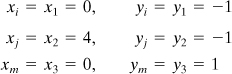
(h)
Using Eq. (7.68) and referring to Fig. 7.26, we obtain
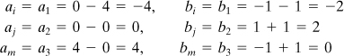
(i)
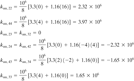
Next, the first equation of (7.76), together with Eqs. (g) and (i), yields
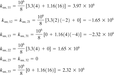
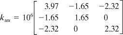
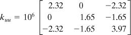
The submatrix kuu is thus
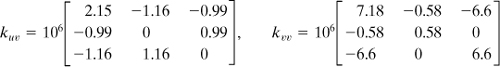
Similarly, from the second and third equations of (7.76), we obtain the following matrices:
Assembling the preceding equations, the stiffness matrix of the element (in newtons per centimeter) is

(j)
b. We next determine the nodal forces of the element owing to various loadings. The components of body force are Fx = 0 and Fy = 0.077 N/cm3.
Body force effects: Through the application of Eq. (7.77), it is found that
![]()
Surface traction effects: The total load, ![]() , is equally divided between nodes 2 and 3. The nodal forces can therefore be expressed as
, is equally divided between nodes 2 and 3. The nodal forces can therefore be expressed as
![]()
Thermal strain effects: The initial strain associated with the 50°C temperature rise is ε0 = αT = 0.0006. From Eq. (7.59),
![]()
Substituting matrix [B], given by Eq. (7.73), into this equation, and the values of the other constants already determined, the nodal force is calculated as follows:
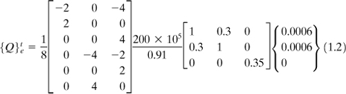
![]()
Equivalent nodal force matrix: Summation of the nodal matrices due to the several effects yields the total element nodal force matrix:

If, in addition, there are any actual node forces, these must also be added to the value obtained.
7.15 Case Studies in Plane Stress
A good engineering case study includes all necessary data to analyze a problem in details and may come in many varieties [Refs. 7.8 and 7.9]. Obviously, in solid mechanics it deals with stress and deformation in load-carrying members or structures. In this section we briefly present four case studies limited to plane stress situations and CST finite elements. A cantilever beam supporting a concentrated load, a deep beam or plate in pure bending, a plate with a hole subjected to an axial loading, and a disk carrying concentrated diametral compression are members considered.
Recall from Chapter 3 that there are very few elasticity or “exact” solutions to two-dimensional problems, especially for any but the simplest shapes. As will become evident from the following discussion, the stress analyst and designer can reach a very accurate solution by employing proper techniques and modeling. Accuracy is often limited by the willingness to model all the significant features of the problem and pursue the FEA until convergence is reached.
Case Study 7.1 Stresses in a Cantilever Beam under a Concentrated Load
Figure 7.27. Case Study 7.1. Cantilever beam (a) before and (b) after being discretized.
Solution


(a)
(b)
and
(c)
(d)
{Q} = {0, 0, 0, 0, 0 –2500, 0 –2500}
u1 = u3 = v1 = v3 = 0
(e)
(f)
(g)

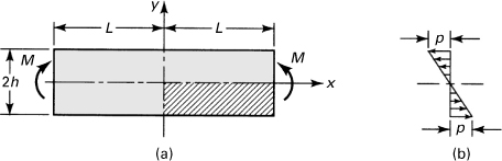
Case Study 7.2 Analysis of a Deep Beam by the Theory of Elasticity and FEM
Figure 7.28. Case Study 7.2. (a) Beam in pure bending; (b) moment is replaced by a statically equivalent load.
Solution
a. Exact solution: Replacing the end moments with the statically equivalent load per unit area p = Mh/I (Fig. 7.28b), the stress distribution from Eq. (5.5) is
(h)
![]()
(i)

(j)
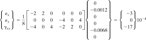
b. Finite element solution: Considerations of symmetry and antisymmetry indicate that only any one-quarter (shown as shaded portion in the figure) of the beam need be analyzed.
![]()
Figure 7.29. Case Study 7.2. Influence of element size and orientation on stress (megapascals) in beam shown in Fig. 7.28.

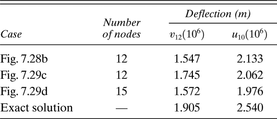
Table 7.4. Comparison of Deflections Obtained by FEM and the Elasticity Theory
Comment
It is clear that we cannot reduce element size to extremely small values, as this would tend to increase to significant magnitudes the computer error incurred. An “exact” solution is thus unattainable, and we seek instead an acceptable solution. The goal is then the establishment of a finite element that ensures convergence to the exact solution in the absence of round-off error. The literature contains many comparisons between the various basic elements. The efficiency of a finite element solution can, in certain situations, be enhanced through the use of a “mix” of elements. For example, a denser mesh within a region of severely changing or localized stress may save much time and effort.
Case Study 7.3 Stress Concentration in a Plate with a Hole in Uniaxial Tension
Figure 7.30. Case Study 7.3. (a) Circular hole in a plate under uniaxial tension; (b) one-quadrant plate model; (c) uniaxial stress (σx) distribution.
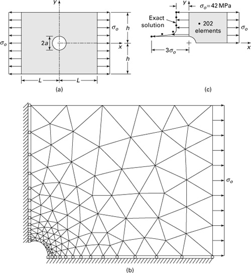
Solution
7.16 Computational Tools
Various computational tools can be employed to carry out analysis calculations with success. A quality scientific calculator may be the best tool for solving most of the problems in this text. General-purpose analysis tools such as spreadsheets and equation solvers are very useful for certain computational tasks. Mathematical software packages of these types include MATLAB, TK Solver, and MathCAD. The tools offer the advantage of allowing the user to document and save the detailed completed work
The computer-aided drafting or design (CAD) software packages can produce realistic three-dimensional representations of a member. Most CAD software provides an interface to one or more FEA programs. They permit direct transfer of the member’s geometry to an FEA package for analysis of stress and vibration as well as fluid and thermal analysis. Computer programs (such as NASTRAN, ANSYS, ABAQUS, GT-STRUDL) are used widely for performing the numerical computations required in the analysis and design of structural and mechanical systems.
With the proper use of computer aided engineering (CAE) software, problems can be solved more quickly and more accurately. Clearly, the results are subject to the accuracy of the various assumptions that must necessarily be made in the analysis and design. The foregoing computer-based software may be used as a tool to assist students with lengthy homework assignments. But it is important that basics be thoroughly understood, and analysts must make checks on computer solutions.
References
7.1. SOKOLNIKOFF, I. S. and REDHEFFER, R. M., Mathematics of Physics and Modern Engineering, 2nd ed., McGraw-Hill, New York, 1966, p. 665.
7.2. YANG, T. Y., Finite Element Structural Analysis, Prentice Hall, Upper Saddle River, N. J., 1986.
7.3. WEAVER, W. JR. and JOHNSTON, P. R., Finite Element for Structural Analysis, Prentice Hall, Upper Saddle River, N. J., 1984.
7.4. GALLAGHER, R. H., Finite Element Analysis: Fundamentals, Prentice Hall, Englewood Cliffs, N. J., 1975.
7.5. MARTIN, H. C. and CAREY, G. F., Introduction to Finite Element Analysis, McGraw-Hill, New York, 1973.
7.6. LOGAN, D. L., A First Course in the Finite Element Method, PWS-Kent, Boston, Mass., 1986.
7.7. KNIGHT, E., The Finite Element Method in Mechanical Design, PWS-Kent, Boston, Mass., 1993.
7.8. UGURAL, A. C., Mechanics of Materials, Wiley, Hoboken, N. J., 2008.
7.9. UGURAL, A. C., Mechanical Design: An Integrated Approach, McGraw-Hill, New York, 2004.
7.10. BORESI, A. P. and SCHMIDT, R. J., Advanced Mechanics of Materials, 6th ed., Wiley, New York, 2003.
7.11. UGURAL, A. C., Stresses in Beams, Plates and Shells, 3rd ed., CRC Press, Taylor & Francis, Boca Raton, Fla. 2010.
7.12. ZIENKIEWICZ, O. C. and TAYLOR, R. I., The Finite Element Method, 4th ed., Vol. 2 (Solid and Fluid Mechanics, Dynamics and Nonlinearity), McGraw-Hill, London, 1991.
7.13. COOK, R. D. and MALKUS, D. S., Concepts and Applications of Finite Element Analysis, 3rd ed., Wiley, Hoboken, N. J., 1989.
7.14. SEGERLIND, L. J., Applied Finite Element Analysis, 2nd ed., Wiley, Hoboken, N. J., 1984.
7.15. BATHE, K. I., Finite Element Procedures in Engineering Analysis, Prentice Hall, Upper Saddle River, N. J., 1996.
7.16. SEGERLIND, L. J., Applied Finite Element Analysis, 2nd ed., Wiley, New York, 1984.
7.17. BAKER, A. J. and PEPPER, D. W., Finite Elements, McGraw-Hill, New York, 1991.
7.18. BERNADOU, M., Finite Element Methods for Thin Shell Problems, Wiley, Chichester, U. K., 1996.
7.19. DUNHAM, R. S. and NICKELL, R. E., “Finite element analysis of axisymmetric solids with arbitrary loadings,” Report AD 655 253, National Technical Information Service, Springfield, Va., June 1967.
7.20. UTKU, S., Explicit expressions for triangular torus element stiffness matrix, AIAA Journal, 6/6, 1174–1176, June 1968.
Problems
Sections 7.1 through 7.4
7.1. Referring to Fig. 7.2, demonstrate that the biharmonic equation
![]()
takes the following finite difference form:
(p7.1)
7.2. Consider a torsional bar having rectangular cross section of width 4a and depth 2a. Divide the cross section into equal nets with h = a/2. Assume that the origin of coordinates is located at the centroid. Find the shear stresses at points x = ±2a and y = ±a. Use the direct finite difference approach. Note that the exact value of stress at y = ±a is, from Table 6.2, τmax = 1.860Gθa.
7.3. For the torsional member of cross section shown in Fig. P7.3, find the shear stresses at point B. Take h = 5 mm and h1 = h2 = 3.5 mm.
7.4. Redo Prob. 7.3 to find the shear stress at point A. Let h = 4.25 mm; then h1 = h and h2 = 2.25 mm.
7.5. Calculate the maximum shear stress in a torsional member of rectangular cross section of sides a and b (a = 1.5b). Employ the finite difference method, taking h = a/4. Compare the results with that given in Table 6.2.
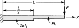
Section 7.5
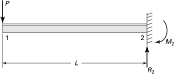
7.6. A force P is applied at the free end of a stepped cantilever beam of length L (Fig. P7.6). Determine the deflection of the free end using the finite difference method, taking n = 3. Compare the result with the exact solution v(L) = 3PL3/16EI.
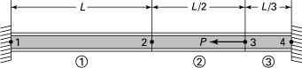
7.7. A stepped simple beam is loaded as shown in Fig. P7.7. Apply the finite difference approach, with h = L/4, to determine (a) the slope at point C; (b) the deflection at point C.
7.8. A stepped simple beam carries a uniform loading of intensity p, as shown in Fig. P7.8. Use the finite difference method to calculate the deflection at point C. Let h = a/2.
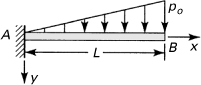
7.9. Cantilever beam AB carries a distributed load that varies linearly as shown in Fig. P7.9. Determine the deflection at the free end by applying the finite difference method. Use n = 4. Compare the result with the “exact” solution w(L) = 11poL4/120EI.
7.10. Applying Eq. (7.22), determine the deflection at points 1 through 5 for beam and loading shown in Fig. P7.10.

7.11. Employ the finite difference method to obtain the maximum deflection and the slope of the simply supported beam loaded as shown in Fig. P7.11. Let h = L/4.
7.12. Determine the deflection at a point B and the slope at point A of the overhanging beam loaded as shown in Fig. P7.12. Use the finite difference approach, with n = 6. Compare the deflection with its “exact” value vB = Pa3/12EI.
7.13. Redo Prob. 7.6 with the beam subjected to a uniform load p per unit length and P = 0. The exact solution is v(L) = 3pL4/32EI.
7.14. A beam is supported and loaded as depicted in Fig. P7.14. Use the finite difference approach, with h = L/4, to compute the maximum deflection and slope.
7.15. A fixed-ended beam supports a concentrated load P at its midspan as shown in Fig. P7.15. Apply the finite difference method to determine the reactions. Let h = L/4.
7.16. Use the finite difference method to calculate the maximum deflection and the slope of a fixed-ended beam of length L carrying a uniform load of intensity p (Fig. P7.16). Let h = L/4.

Sections 7.6 through 7.16
7.17. The bar element 4–1 of length L and the cross-sectional area A is oriented at an angle α clockwise from the x axis (Fig. P7.17). Calculate (a) the global stiffness matrix of the bar; (b) the axial force in the bar; (c) the local displacements at the ends of the bar. Given: A = 1350 mm2, L = 1.7 m, α = 60°, E = 96 GPa, u4 = –1.1 mm, v4 = –1.2 mm, u1 = 2 mm, and v1 = 1.5 mm.
7.18. The axially loaded bar 1–4 of constant axial rigidity AE is held between two rigid supports and under a concentrated load P at node 3, as illustrated in Fig. P7.18. Find (a) the system stiffness matrix; (b) the displacements at nodes 2 and 3; (c) the nodal forces and reactions at the supports.
7.19. The axially loaded composite bar 1–4 is held between two rigid supports and subjected to a concentrated load P at node 2, as depicted in Fig. P7.19. The steel bar 1–3 has cross-sectional area A and modulus of elasticity E. The brass bar 3–4 is with cross-sectional area 2A and elastic modulus E/2. Determine (a) the system stiffness matrix; (b) the displacements of nodes 2 and 3; (c) the nodal forces and reactions at the supports.

7.20. A stepped bar 1–4 is held between rigid supports and carries a concentrated load P at node 3, as illustrated in Fig. P7.20. Find (a) the system stiffness matrix; (b) the displacements of nodes 2 and 3; (c) the nodal forces and reactions at the supports.
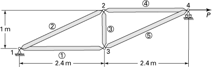
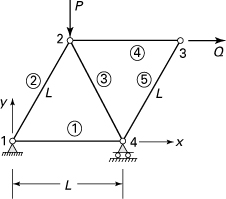
7.21. A planar truss containing five members with axial rigidity AE is supported at joints 1 and 4, as shown in Fig. P7.21. What is the global stiffness matrix for each element?
7.22. The plane truss is loaded and supported as illustrated in Fig. P7.22. Each element has an axial rigidity AE. Find (a) the global stiffness matrix for each element; (b) the system stiffness matrix; (c) the system force-displacement relations.
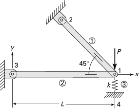
7.23. A two-bar planar truss is supported by a spring of stiffness k at joint 1, as depicted in Fig. P7.23. Each element has an axial rigidity AE. Calculate (a) the stiffness matrix for bars 1 and 2, and spring 3; (b) the system stiffness matrix; (c) the force-displacement equations. Given: L2 = L, (AE)2 = AE, ![]() ,
, ![]() .
.
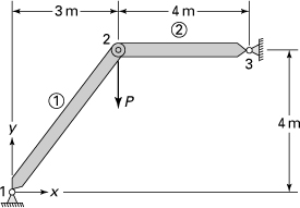
7.24. A vertical concentrated load P = 6 kN is applied at joint 2 of the two-bar plane truss supported as shown in Fig. P7.24. Take AE = 20 MN for each member. Find (a) the global stiffness matrix of each bar; (b) the system stiffness matrix; (c) the nodal displacements; (d) the support reactions; (e) the axial forces in each bar.

7.25. In a two-bar plane truss, its support at joint 1 settles vertically by an amount of u = 15 mm downward when loaded by a horizontal concentrated load P (Fig. P7.25). Calculate (a) the global stiffness matrix of each element; (b) the system stiffness matrix; (c) the nodal displacements; (d) the support reactions. Given: E = 105 GPa, A = 10 × 10–4 m2, P = 10 kN.

7.26. A cantilever of constant flexural rigidity EI carries a concentrated load P at its free end, as shown in Fig. P7.26. Find (a) the deflection v1 and angle of rotation θ1 at the free end; (b) the reactions R2 and M2 at the fixed end.
7.27. A simple beam 1–3 of length L and flexural rigidity EI is supports a uniformly distributed load of intensity p, as illustrated in Fig. P7.27. Determine the deflection of the beam at midpoint 2 by replacing the applied load with the equivalent nodal loads (see Table D.5).

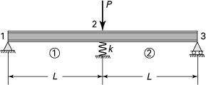
7.28. A beam supported by a pin, a spring of stiffness k, and a roller at points 1, 2, and 3, respectively, is under a concentrated load P at point 2 (Fig. P7.28). Calculate (a) the nodal displacements; (b) the nodal forces and spring force. Given: L = 4 m, P = 12 kN, EI = 14 MN · m2, and k = 200 kN/m.
7.29. A cantilever beam 1–2 of length L and constant flexural rigidity EI is subjected to a concentrated load P at the midspan, as shown in Fig. P7.29. Find the vertical deflection v2 and angle of rotation θ2 at the free end by replacing the applied load with the equivalent nodal loads acting at each end of the beam (see Table D.5).

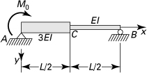
7.30. A propped cantilever beam with flexural rigidities EI and EI/2 for the parts 1–2 and 2–3, respectively, carries concentrated load P and moment 3PL at point 2 (Fig. P7.30). Calculate the displacements v2, θ2, and θ3. Given: L = 1.2 m, P = 30 kN, E = 207 GPa, and I = 15 × 106 mm4.

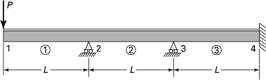
7.31. A continuous beam of constant flexural rigidity EI is loaded and supported as seen in Fig. P7.31. Determine (a) the stiffness matrix for each element; (b) the system stiffness matrix and the force-displacement relations.
7.32. A propped cantilever beam with an overhang is subjected to a concentrated load P, as illustrated in Fig. P7.32. The beam has a constant flexural rigidity EI. Determine (a) the stiffness matrix for each element; (b) the system stiffness matrix; (c) the nodal displacements; (d) the forces and moments at the ends of each member; (e) the shear and moment diagrams.

7.33. A plane truss consisting of five members having the same axial rigidity AE is supported at joints 1 and 4, as seen in Fig. P7.33. Find the global stiffness matrix for each element.
7.34. The planar truss, with the axial rigidity AE the same for each element, is loaded and supported as illustrated in Fig. P7.34. Determine (a) the global stiffness matrix for each element; (b) the system matrix and the system force-displacement equations.
7.35. A vertical load P = 20 kN acts at joint 2 of the two-bar (1–2 and 2–3) truss shown in Fig. P7.35. Find (a) the global stiffness matrix for each member; (b) the system stiffness matrix; (c) the nodal displacements; (d) reactions; (e) the axial forces in each member, and show the results on a sketch of each member. Assumption: The axial rigidity AE = 60 MN is the same for each bar.
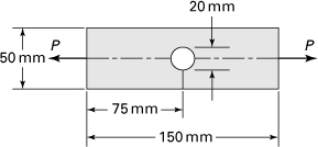
7.36. A plate with a hole is under an axial tension loading P (Fig. P7.36). Dimensions are in millimeters. Given: P = 5 kN and plate thickness t = 12 mm. (a) Analyze the stresses using a computer program with the CST (or LST) elements. (b) Compare the stress concentration factor K obtained in part (a) with that found from Fig. D.8.
7.37. Resolve Prob. 7.36 for the plate shown in Fig. P7.37.

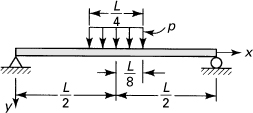
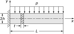
7.38. A simple beam is under a uniform loading of intensity p (Fig. P7.38). Let L = 10h, t = 1, and v = 0.3. Refine meshes to calculate the stress and deflection within 5% accuracy, by using a computer program with the CST (or LST) elements. Given: Exact solution [Ref. 7.7] is of the form:
(p7.38)
where t represents the thickness.
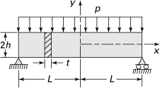
7.39. Resolve Prob. 7.38 for the case in which a cantilever beam is under a uniform loading of intensity p (Fig. P7.39). Given: Exact solution [Ref. 7.7] is given by
(p7.39)
in which t is the thickness.
7.40. Verify Eqs. (7.78) and (7.79) by determining the static resultant of the applied loading. [Hint: For Eq. (7.79), apply the principle of virtual work.]
![]()
with
![]()
to obtain
![]()
7.41. Redo Case Study 7.1 for the beam subjected to a uniform additional load throughout its span, p = –7 MPa, and a temperature rise of 50°C. Let γ = 77 kN/m3 and α = 12 × 10–6/°C.
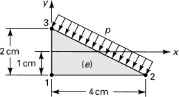
7.42. A ![]() -cm-thick cantilever beam is subjected to a parabolically varying end shear stress resulting in a load of P N and a linearly distributed load p N/cm (Fig. P7.42). Dividing the beam into two triangles as shown, calculate the stresses in the member. The beam is made of a transversely isotropic material, in which a rotational symmetry of properties exists within the xz plane:
-cm-thick cantilever beam is subjected to a parabolically varying end shear stress resulting in a load of P N and a linearly distributed load p N/cm (Fig. P7.42). Dividing the beam into two triangles as shown, calculate the stresses in the member. The beam is made of a transversely isotropic material, in which a rotational symmetry of properties exists within the xz plane:
![]()
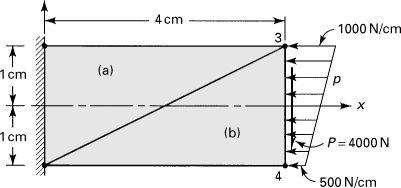
Here E1 is associated with the behavior in the xz plane, and E2, G2, and v2 with the direction perpendicular to the xz plane. Now the elasticity matrix, Eq. (7.54), becomes
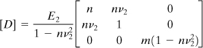
where n = E1/E2 and m = G2/E2.
7.43. Redo Case Study 7.1 if the discretized beam consists of triangular elements 1 4 3 and 1 2 4 (Fig. 7.27b). Assume the remaining data to be unchanged.