Chapter 11. Stability of Columns
11.1 Introduction
We have up to now dealt primarily with the prediction of stress and deformation in structural elements subject to various load configurations. Failure criteria have been based on a number of theories relying on the attainment of a particular stress, strain, or energy level within the body. This chapter demonstrates that the beginnings of structural failure may occur prior to the onset of any seriously high levels of stress. We thus explore failure owing to buckling or elastic instability and seek to determine those conditions of load and geometry that lead to a compromise of structural integrity.
We are concerned only with beams and slender members subject to axial compression. The problem is essentially one of ascertaining those configurations of the system that lead to sustainable patterns of deformation. The principal difference between the theories of linear elasticity and linear stability is that, in the former, equilibrium is based on the undeformed geometry, whereas in the latter the deformed geometry must be considered. Our treatment primarily concerns ideal columns. We define an ideal column as a perfectly constructed, perfectly straight column that is built of material that follows Hooke’s law and that is under centric loading. Practical formulas and graphs are presented to facilitate improved understanding of the behavior of both elastic and inelastic actual columns.
11.2 Critical Load
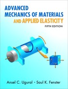
To demonstrate the concepts of stability and critical load, consider the idealized structure: a rigid, weightless bar AB, shown in Fig. 11.1a. This member is pinned at B and acted on by a force P. In the absence of restoring influences such as the spring shown, any small lateral disturbance (causing a displacement δ) will result in rotation of the bar, as illustrated in Fig. 11.1b, with no possibility of return to the original configuration. Without the spring, therefore, the situation depicted in the figure is one of unstable equilibrium. With a spring present, different possibilities arise.
Figure 11.1. Buckling behavior of a rigid bar: (a) vertical configuration; (b) displacement configuration; (c) equilibrium diagram.

Equilibrium Method
A small momentary disturbance δ can now be sustained by the system (provided that P is also small) because the disturbing moment Pδ is smaller than the restoring moment FL = kδL (where k represents the linear spring constant, force per unit of deformation). For a small enough value of P, the moment kδL will thus be sufficient to return the bar to δ = 0. Since the system reacts to a small disturbance by creating a counterbalancing effect acting to diminish the disturbance, the configuration is in stable equilibrium.
If now the load is increased to the point where
(a)
it is clear that any small disturbance δ will be neither diminished nor amplified. The system is now in neutral equilibrium at any small value of δ. Expression (a) defines the critical load:
(b)
If P > Pcr, the net moment acting will be such as to increase δ, tending to further increase the disturbing moment Pδ, and so on. For P > Pcr, the system is in unstable equilibrium because any lateral disturbance will be amplified, as in the springless case discussed earlier.
The equilibrium regimes are shown in Fig. 11.1c. Note that C, termed the bifurcation point, marks the two branches of the equilibrium solution. One is the vertical branch (P ≤ Pcr, δ = 0), and the other is the horizontal (P = Pcr, δ > 0).
Energy Method
Stability may also be interpreted in terms of energy concepts, however. Referring again to Fig. 11.1b, the work done by P as it acts through a distance L(1 – cos θ) is

The elastic energy acquired as a result of the corresponding spring elongation Lθ is
![]()
If ΔU > ΔW, the configuration is stable; the work done is insufficient to result in a displacement that grows subsequent to a lateral disturbance. However, if ΔW > ΔU, the system is unstable because now the work is large enough to cause the displacement to grow following a disturbance. The boundary between stable and unstable configurations corresponds to ΔW = ΔU,
Pcr = kL
as before.
The buckling analysis of compression members usually follows in essentially the same manner. Either the static equilibrium or the energy approach may be used for determination of the critical load. The choice depends on the particulars of the situation under analysis. Although the static equilibrium method leads to exact solutions, the results offered by the energy approach (sometimes approximate) are often preferable because of the physical insights that may be more readily gained.
11.3 Buckling of Pinned-End Columns
Consideration is now given to a relatively slender straight bar subject to axial compression. This member, a column, is similar to the element shown in Fig. 11.1a, in that it too can experience unstable behavior. In the case of a column, the restoring force or moment is provided by elastic forces established within the member rather than by springs external to it.
Refer to Fig. 11.2a, in which is shown a straight, homogeneous, pin-ended column. For such a column, the end moments are zero. This is regarded as the fundamental or most basic case. It is reasonable to suppose that the column can be held in a deformed configuration by a load P while remaining in the elastic range (Fig. 11.2b). Note that the requisite axial motion is permitted by the movable end support. In Fig. 11.2c, the postulated deflection is shown, having been caused by collinear forces P acting at the centroid of the cross section. The bending moment at any section, M = –Pv, when inserted into the equation for the elastic behavior of a beam, EIv″ = M, yields
(11.1)
Figure 11.2. Pinned-end column: (a) initial form; (b) buckled form; (c) free-body diagram of column segment.
The solution of this differential equation is
(a)
where the constants of integration, c1 and c2, are determined from the end conditions: v(0) = v(L) = 0. From v(0) = 0, we find that c2 = 0. Substituting the second condition into Eq. (a), we obtain
(b)
It must be concluded that either c1 = 0, in which case v = 0 for all x and the column remains straight regardless of load, or sin ![]() . The case of c1 = 0 corresponds to a condition of no buckling and yields a trivial solution [the energy approach (Sec. 11.10) sheds further light on this case]. The latter is the acceptable alternative because it is consistent with column deflection. It is satisfied if
. The case of c1 = 0 corresponds to a condition of no buckling and yields a trivial solution [the energy approach (Sec. 11.10) sheds further light on this case]. The latter is the acceptable alternative because it is consistent with column deflection. It is satisfied if
(c)
The value of P ascertained from Eq. (c), that is, the load for which the column may be maintained in a deflected shape, is the critical load,
(11.2)
where L represents the original length of the column. Assuming that column deflection is in no way restricted to a particular plane, the deflection may be expected to occur about an axis through the centroid for which the second moment of area is a minimum. The lowest critical load or Euler buckling load of the pin-ended column is of greatest interest; for n = 1,
The preceding, after L. Euler (1707–1783), represents the maximum theoretical load that an idealized column can expect to resist. Recall that a centrically loaded column in which the deflections are small, the construction is perfect, and the material follows Hooke’s law is called an ideal column.
The deflection is found by combining Eqs. (a) and (c) and inserting the values of c1 and c2:
(11.4)
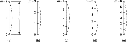
in which c1 represents the amplitude of the elastic curve. It is noted that a slender pin-ended elastic column has more than one critical load, as indicated in Eq. (11.2). When the column is restrained from buckling into a single lobe by a lateral support, it may buckle at a load higher than Pcr. A column with pinned ends can buckle in the shape of a single sine lobe (n = 1) at the critical load Pcr. But if it is prevented from bending in the form of one lobe by one lateral support, the load can increase until it buckles into two lobes (n = 2). Applying Eq. (11.2), for n = 2, the critical load is (Pcr)2 = 4(π2EI/L) = 4Pcr. Figure 11.3 illustrates the buckling modes for n = 1 and 2. The higher buckling modes (n = 3, ...) are sketched similarly. Observe that, as n increases, the number of nodal points and critical buckling load also increase. However, usually the lowest buckling mode is significant.
Figure 11.3. First two buckling modes for a pin-ended column.

We conclude this section by recalling that the boundary conditions employed in the solution of the differential equation led to an infinite set of discrete values of load, (Pcr)n. These solutions, typical of many engineering problems, are termed eigenvalues, and the corresponding deflections v are the eigenfunctions.
11.4 Deflection Response of Columns
The conclusions of the preceding section are predicated on the linearized beam theory with which the analysis began. Recall from Section 5.2 that, in Eq. (11.1), the term d2v/dx2 is actually an approximation to the curvature. Inasmuch as c1 in Eq. (11.4) is undefined (and independent of Pcr), the critical load and deflection are independent, and Pcr will sustain any small lateral deflection, a condition represented by the horizontal line AB in Fig. 11.4. It is clear that, in this figure, we show only the right-hand half of the diagram; however, the two halves are symmetric about the vertical axis. Note that the effects of temperature and time on buckling are not considered in the following discussion. Essentially, these effects may be very significant and often act to lower the critical load.
Figure 11.4. Relation between load and deflection for columns.

Effects of Large Deflections
Were the exact curvature used, the differential equation derived would apply to large deformations within the elastic range, and the result would be less restricted. For this case, it is found that P depends on the magnitude of the deflection or c1. Exact or large deflection analysis also reveals values of P exceeding Pcr, as shown with the curve AC in Fig. 11.4. That is, after an elastic column begins to buckle, a larger and larger load is required to cause an increase in the deflections. However, the bending stresses accompanying large deflection could carry the material into inelastic regime, thus leading to diminishing buckling loads [Ref. 11.1]. So, the load-deflection curve AC drops (as indicated by the dashed lines), and the column fails either by excessive yielding or fracture. Thus, in most applications, Pcr is usually regarded as the maximum load sustainable by a column.
Effects of Imperfections
The column that poses deviations from ideal conditions assumed in the preceding is called an imperfect column. Such a column is not constructed perfectly; for example, it could have an imperfection in the form of a misalignment of load or a small initial curvature or crookedness (see Secs. 11.8 and 11.9). An imperfection produces deflections from the start of loading, as depicted by curve OD in Fig. 11.4. For the case in which deflections are small, curve OD approaches line AB; as the deflections become large, it approaches curve AC. The larger the imperfections, the further curve OD moves to the right. For the case in which the column is constructed with great accuracy, curve OD approaches more closely to the straight lines OA and AB. Observe from these lines and curves AC and OD that Pcr represents the maximum load-carrying capacity of an elastic column for practical purposes, because large deflections generally are not permitted to occur in structures.
Effects of Inelastic Behavior
We now consider the situation where the stresses exceed the proportional limit and the column material no longer follows Hooke’s law. Obviously, the load-deflection curve is unchanged up to the level of load at which the proportional limit is reached. Then the curve for inelastic behavior (curve OE) deviates from the elastic curve, continues upward, reaches a maximum, and turns downward, as seen in Fig. 11.4. The specific forms of these curves depend on the material properties and column dimensions; however, the usual nature of the behavior is exemplified by the curves depicted. Empirical methods are often used in conjunction with analysis to develop an efficient design criteria.
Very slender columns alone remain elastic up to the critical load Pcr. If the load is slightly eccentric, a slender column will undergo lateral deflection as soon as load is applied. For intermediate columns, instability and inelastic collapse take place at relatively small lateral deflections. Short columns behave inelastically and follow a curve such as OD. Observe that the maximum load P that can be carried by an inelastic column may be considerably less than the critical load Pcr. A final point to note is that the descending part of curve OE leads to a plastic collapse or fracture, because it takes smaller and smaller loads to maintain larger and larger deflections. On the contrary, the curves for elastic columns are quite stable, since they continue upward as the deflections increase. Thus, it takes larger and larger loads to produce an increase in deflection.
11.5 Columns with Different End Conditions
It is evident from the foregoing derivation that Pcr depends on the end conditions of the column. For other than the pin-ended, fundamental case discussed, we need only substitute the appropriate conditions into Eq. (a) of Section 11.3 and proceed as before.
Consider an alternative approach, beginning with the following revised form of the Euler buckling formula for a pin-ended column and applicable to a variety of end conditions:
(11.5)
Here Le denotes the effective column length, which for the pin-ended column is the column length L. The effective length, shown in Fig. 11.5 for several end conditions, is determined by noting the length of a segment corresponding to a pin-ended column. In so doing we seek the distance between points of inflection on the elastic curve or the distance between hinges, if any exist.
Figure 11.5. Effective lengths of columns with different restraints: (a) fixed-free; (b) pinned-pinned; (c) fixed-pinned; (d) fixed-fixed.

Regardless of end condition, it is observed that the critical load depends not on material strength but on the flexural rigidity, EI. Buckling resistance can thus be enhanced by deploying material so as to maximize the moment of inertia, but not to the point where the section thickness is so small as to result in local buckling or wrinkling. Setting I = Ar2, the preceding equation may be written as
(11.6)
where A is the cross-sectional area and r is the radius of gyration. The quantity Le/r, called the effective slenderness ratio, is an important parameter in the classification of compression members.
Example 11.1. Load-Carrying Capacity of a Wood Column
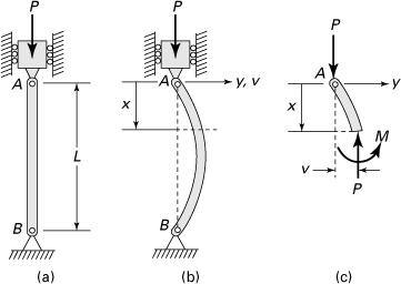
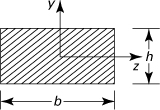
A pinned-end wood bar of width b by depth h rectangular cross section (Fig. 11.6) and length L is subjected to an axial compressive load. Determine (a) the slenderness ratio; (b) the allowable load, using a factor safety of n. Data: b = 60 mm, h = 120 mm, L = 1.8 m, n = 1.4, E = 12 GPa, and σu = 55 MPa (by Table D.1).
Figure 11.6. Example 11.1. Cross section of wooden column.
Solution
The properties of the cross-sectional area are A = bh, Ix = hb3/12, Iy = hb3/12, and ![]() .
.
a. Slenderness ratio: The smallest value of r is found when the centroidal axis is parallel to the longer side of the rectangle. Therefore,
(a)
Substituting the given numerical value, we obtain
![]()
Since L = Le, it follows that
![]()
b. Permissible load: Applying Eq. (11.6), the Euler buckling load with ry = r and A = 60 × 120 = 7.2 × 103 mm2 is
![]()
Comment
The largest load the column can support equals, then, P = 79/1.4 = 56.4 kN. Observe that, based on material strength, the allowable load equals
![]()
This, compared with 56.4 kN, shows the importance of buckling analysis in predicting the safe working load.
11.6 Critical Stress: Classification of Columns
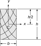
The behavior of an ideal column is often represented on a plot of average compressive stress P/A versus slenderness ratio Le/r (Fig. 11.7). Such a representation offers a clear rationale for the classification of compression bars. Tests of columns verify each portion of the curve with reasonable accuracy. The range of Le/r is a function of the material under consideration. We note that the regions AB, BC, and CD represent the strength limit in compression, inelastic buckling limit, and elastic buckling limit, respectively.
Figure 11.7. Critical stress versus slenderness ratio.
Long Columns
For a member of sufficiently large slenderness ratio or long column, buckling occurs elastically at a stress that does not exceed the proportional limit of the material.
Consequently, the Euler’s load of Eq. (11.6) is appropriate to this case. The critical stress is therefore
(11.7)
The associated portion CD of the curve (Fig. 11.7) is labeled as Euler’s curve. The critical value of slenderness ratio that fixes the lower limit of this curve, found by equating σcr to the proportional limit (σpl) of the specific material, is given by
(a)
In the case of a structural steel with modulus of elasticity E = 210 GPa and yield strength σyp ≈ σpl = 250 MPa (Table D.1), for instance, the foregoing gives (Le/r)c = 91.
It is seen from Fig. 11.7 that very slender columns buckle at low levels of stress; they are much less stable than short columns. Use of a higher strength material does not improve this situation. Interestingly, Eq. (11.7) shows that the critical stress is increased by using a material of higher modulus elasticity E or by increasing the radius of gyration r.
Short Columns
Compression members having low slenderness ratios (for example, steel rods with L/r < 30) exhibit essentially no instability and are referred to as short columns or struts. For these bars, failure occurs by crushing, without buckling, at stresses exceeding the proportional limit of the material. The maximum stress is thus
(11.8)
This represents the strength limit of a short column, represented by horizontal line AB in Fig. 11.7. Clearly, it is equal to the ultimate stress in compression.
Intermediate Columns: Inelastic Buckling
Most structural columns lie in a region between short and long classifications represented by the part BC in Fig. 11.7. Such intermediate-length columns* do not fail by direct compression or by elastic instability. Hence, Eqs. (11.7) and (11.8) do not apply, and a separate analysis is required. The failure of an intermediate column occurs by inelastic buckling at stress levels exceeding the proportional limit. Over the years, numerous empirical formulas have been developed for the intermediate slenderness ratios. Presented here are two practical methods for finding critical stress in inelastic buckling.
Tangent Modulus Theory
Consider the concentric compression of an intermediate column, and imagine the loading to occur in small increments until such time as the buckling load Pt is achieved. As we would expect, the column does not remain perfectly straight but displays slight curvature as the increments in load are imposed. It is fundamental to the tangent modulus theory to assume that accompanying the increasing loads and curvature is a continuous increase, or no decrease, in the longitudinal stress and strain in every fiber of the column. That this should happen is not at all obvious, for it is reasonable to suppose that fibers on the convex side of the member might elongate, thereby reducing the stress. Accepting the former assumption, the stress distribution is as shown in Fig 11.8a. The increment of stress, Δσ, is attributable to bending effects; σcr is the value of stress associated with the attainment of the critical load Pt. The distribution of strain will display a pattern similar to that shown in Fig. 11.8b.
Figure 11.8. (a) Stress distribution for tangent-modulus load; (b) stress–strain diagram.

For small deformations Δv, the increments of stress and strain will likewise be small, and as in the case of elastic bending, sections originally plane are assumed to remain plane subsequent to bending. The change of stress Δσ is thus assumed proportional to the increment of strain, Δε; that is, Δσ = Et Δε. The constant of proportionality Et is the slope of the stress–strain diagram beyond the proportional limit, termed the tangent modulus (Fig. 11.8b). Note that within the linearly elastic range, Et = E. The stress–strain relationship beyond the proportional limit during the change in strain from ε to ε + Δε is thus assumed linear, as in the case of elastic buckling. The critical or Engesser stress may, on the basis of the foregoing rationale, be expressed by means of a modification of Eq. (11.6) in which Et replaces E. Hence the critical stress may be expressed by the generalized Euler buckling formula, or the tangent modulus formula:
(11.9)
This is the so-called Engesser formula, proposed by F. Engesser in 1889. The buckling load Pt predicted by Eq. (11.9) is in good agreement with test results and therefore recommended for design purposes [Ref. 11.2].
When the critical stress is known and the slenderness ratio required, the application of Eq. (11.9) is straightforward. The value of Et corresponding to σcr is read from the stress–strain curve obtained from a simple compression test, following which Le/r is calculated using Eq. (11.9). If, however, Le/r is known and σcr is to be ascertained, a trial-and-error approach is necessary (see Prob. 11.20).
Johnson’s Buckling Criterion
Many formulas are based on the use of linear or parabolic relationship between the slenderness ratio and the critical stress for intermediate columns. The most widely employed modification of the parabola, proposed by J. B. Johnson around 1900, is the Johnson formula:
(11.10a)
In terms of the critical load, we write
(11.10b)
where A is the cross-sectional area of the column. The Johnson’s equation has been found to agree reasonably well with experimental results. But the dimensionless form of tangent modulus curves have very distinct advantages when structures of new materials are analyzed [Refs. 11.3 and 11.4].
Specific Johnson formula for regular cross-sectional shapes may be developed by substituting pertinent values of radius of gyration r and area A into Eq. (11.10). It can be readily shown that (see Prob. 11.8), in case of a solid circular section of diameter d:
(11.11)
Likewise, for a rectangular section of height h and depth b:
(11.12)
in which, it is assumed that h ≤ b.
We note that Eqs. (11.7) through (11.10) determine the ultimate stresses, not the working stresses. It is thus necessary to divide the right side of each formula by an appropriate factor of safety, usually 2 to 3, depending on the material, in order to obtain the allowable values. Some typical relationships for allowable stress are introduced in the next section.
11.7 Allowable Stress
The foregoing discussion and analysis have related to ideal, homogeneous, concentrically loaded columns. Inasmuch as such columns are not likely candidates for application in structures, actual design requires the use of empirical formulas based on a strong background of test and experience. Care must be exercised in applying such special-purpose formulas. The designer should be prepared to respond to the following questions:
To what material does the formula apply?
Does the formula already contain a factor of safety, or is the factor of safety separately applied?
For what range of slenderness ratios is the formula valid?
Included among the many special-purpose relationships developed are the following, recommended by the American Institute of Steel Construction (AISC) and valid for a structural steel column:*

(11.13)
Here σall, σyp, Cc, and n denote, respectively, the allowable and yield stresses, a material constant, and the factor of safety. The values of Cc and n are given by
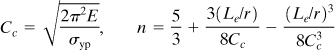
(11.14)
This relationship provides a smaller n for a short strut than for a column of higher Le/r, recognizing that the former fails by yielding and the latter by buckling. The use of a variable factor of safety provides a consistent buckling formula for various ranges of Le/r. The second equation of (11.13) includes a constant factor of safety and gives the value of allowable stress in pascals. Both formulas apply to principal load-carrying (main) members.
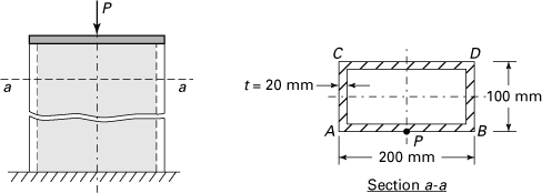
Example 11.2. Buckling of the Boom of a Crane
The boom of a crane, shown in Fig. 11.9, is constructed of steel, E = 210 GPa; the yield point stress is 250 MPa. The cross section is rectangular with a depth of 100 mm and a thickness of 50 mm. Determine the buckling load of the column.
Figure 11.9. Example 11.2. A boom and cable assembly carrying a load W.

Solution
The moments of inertia of the section are Iz = 0.05(0.1)3/12 = 4.17 × 10⁻⁶ m4 and Iy = 0.1(0.05)3/12 = 1.04 × 10⁻⁶ m4. The least radius of gyration is thus ![]() , and the slenderness ratio is L/r = 194. The Euler formula is applicable in this range. From statics, the axial force in terms of W is P = W/tan 15° = 3.732W. Applying the formula for a hinged-end column, Eq. (11.5), for buckling in the yx plane, we have
, and the slenderness ratio is L/r = 194. The Euler formula is applicable in this range. From statics, the axial force in terms of W is P = W/tan 15° = 3.732W. Applying the formula for a hinged-end column, Eq. (11.5), for buckling in the yx plane, we have
![]()
or
W = 305.9 kN
To calculate the load required for buckling in the xz plane, we must take note of the fact that the line of action of the compressive force passes through the joint and thus causes no moment about the y axis at the fixed end. Therefore, Eq. (11.5) may again be applied:
![]()
or
W = 76.3 kN
The member will thus fail by lateral buckling when the load W exceeds 76.3 kN. Note that the critical stress Pcr/A = 76.3/0.005 = 15.26 MPa. This, compared with the yield strength of 250 MPa, indicates the importance of buckling analysis in predicting the safe working load.
11.8 Imperfections in Columns
As might be expected, the load-carrying capacity and deformation under load of a column are significantly affected by even a small initial curvature (see Fig. 11.4). In the preceding section, we described how to account for the effects of imperfections in construction of the column. To ascertain the extent of this influence, consider a pin-ended column for which the unloaded shape is described by
(a)
as shown by the dashed lines in Fig. 11.10. Here ao is the maximum initial deflection, or crookedness of the column. An additional deflection v1 will accompany a subsequently applied load P, so the total deflection is
(b)
Figure 11.10. (a) Initially curved column with pinned ends; (b) the cross section.
The differential equation of the column is thus
(c)
which together with Eq. (a) becomes
![]()
When the trial particular solution
![]()
is substituted into Eq. (c), it is found that
(d)
The general solution of Eq. (c) is therefore
(e)
The constants c1 and c2 are evaluated upon consideration of the end conditions v1(0) = v1(L) = 0. The result of substituting these conditions is c1 = c2 = 0; the column deflection is thus
(11.15)
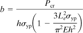
As for the critical stress, we begin with the expression applicable to combined axial loading and bending: σx = (P/A) ± (My/I), where A and I are the cross-sectional area and the moment of inertia. On substitution of Eqs. (c) and (11.15) into this expression, the maximum compressive stress at midspan is found to be
(11.16)
Here S is the section modulus I/c, where c represents the distance measured in the y direction from the centroid of the cross section to the extreme fibers. In Eq. (11.16), σmax is limited to the proportional or yield stress of the column material. Thus, setting σmax = σyp and P = PL, we rewrite Eq. (11.16) as follows:
(11.17)
where PL is the limit load that results in impending yielding and subsequent failure. Given σyp, ao, E, and the column dimensions, Eq. (11.17) may be solved exactly by solving a quadratic or by trial and error for PL. The allowable load Pall can then be found by dividing PL by an appropriate factor of safety, n. Interestingly, in Eqs. (11.16) and (11.17), the term ao A/S = aoc/r2 is known as the imperfection ratio, where r is the radius of gyration. Another approach to account for the effect of imperfections due to eccentricities in the line of application of the load is discussed in the next section.
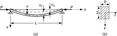
11.9 Eccentrically Loaded Columns: Secant Formula
In contrast with the cases considered up to this point, we now analyze columns that are loaded eccentrically, that is, those in which the load is not applied at the centroid of the cross section. This situation is clearly of great practical importance, since we ordinarily have no assurance that loads are truly concentric. As seen in Fig. 11.11a, the bending moment at any section is –P(v + e), where e is the eccentricity, defined in the figure. It follows that the beam equation is given by
(a)
or
![]()
Figure 11.11. (a) Eccentrically loaded column; (b) graph of secant formula.
The general solution is
(b)
To determine the constants c1 and c2, the end conditions v(L/2) = v(–L/2) = 0 are applied, with the result
![]()
Substituting these values into Eq. (b) provides an expression for the column deflection:
(c)
In terms of the critical load Pcr = π2EI/L2, the midspan deflection is
(11.18)
As P approaches Pcr, the maximum deflection is thus observed to approach infinity.
The maximum compressive stress, (P/A) + (Mc/I), occurs at x = 0 on the concave side of the column; it is given by the so-called secant formula:
(11.19)
where r represents the radius of gyration and c is the distance from the centroid of the cross section to the extreme fibers, both in the direction of eccentricity. When the eccentricity is zero, this formula no longer applies. Then, we have an ideal column with centric loading, and Eq. (11.7) is to be used.
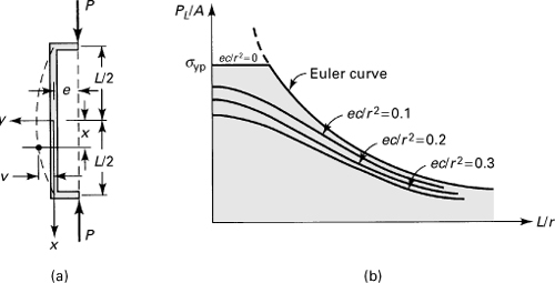
Expression (11.19) gives σmax in the column as a function of the average stress (P/A), the eccentricity ratio (ec/r2), and the slenderness ratio (L/r). As in the case of initially curved columns, if we let σmax = σyp and the limit load P = PL, Eq. (11.19) becomes
(11.20)
For any prescribed yield stress and eccentricity ratio, Eq. (11.20) can be solved by trial and error, or by a root-finding technique using numerical methods, and PL/A plotted as a function of L/r with E held constant (Fig. 11.11b). The allowable value of the average compressive load is found from Pall = PL/n. The development on which Eq. (11.19) is based assumes buckling to occur in the xy plane. It is also necessary to investigate buckling in the xz plane, for which Eq. (11.19) does not apply. This possibility relates especially to narrow columns.
The behavior of a beam subjected to simultaneous axial and lateral loading, the beam column, is analogous to that of the bar shown in Fig. 11.1a, with an additional force acting transverse to the bar. For problems of this type, energy methods are usually more efficient than the equilibrium approach previously employed.
11.10 Energy Methods Applied to Buckling
Energy techniques usually offer considerable ease of solution compared with equilibrium approaches to the analysis of elastic stability and the determination of critical loads. Recall from Chapter 10 that energy methods are especially useful in treating members of variable cross section, where the variation can be expressed as a function of the beam axial coordinate.
To illustrate the method, let us apply the principle of virtual work in analyzing the stability of a straight, pin-ended column. Locate the origin of coordinates at the stationary end. Recall from Section 10.8 that the principle of virtual work may be stated as
(a)
where W and U are the virtual work and strain energy, respectively. Consider the configuration of the column in the first buckling mode, denoting the arc length of a column segment by ds. The displacement, δu = ds – dx, experienced by the column in the direction of applied load P is given by Eq. (10.29). Since the load remains constant, the work done is therefore
(11.21)
Next, the strain energy must be evaluated. There are components of strain energy associated with column bending, compression, and shear. We shall neglect the last. From Eq. (5.62), the bending component is
The energy due to a uniform compressive loading P is, according to Eq. (2.59),
(11.23)
Inasmuch as U2 is constant, it plays no role in the analysis. The change in the strain energy as the column proceeds from its original to its buckled configuration is therefore
(b)
since the initial strain energy is zero. Substituting Eqs. (11.21) and (b) into Eq. (a), we have
(11.24a)
from which

(11.24b)
This result applies to a column with any end condition. The end conditions specific to this problem will be satisfied by a solution
![]()
where a1 is a constant. After substituting this assumed deflection into Eq. (11.24b) and integrating, we obtain
![]()
The minimum critical load and the deflection to which this corresponds are
(c)
It is apparent from Eq. (11.24a) that for P > Pcr, the work done by P exceeds the strain energy stored in the column. The assertion can therefore be made that a straight column is unstable when P > Pcr. This point, with regard to stability, corresponds to c1 = 0 in Eq. (b) of Section 11.3; it could not be obtained as readily from the equilibrium approach. In the event that P = Pcr, the column exists in neutral equilibrium. For P < Pcr, a straight column is in stable equilibrium.
Example 11.3. Deflection of a Beam Column
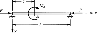
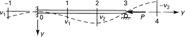
A simply supported beam is subjected to a moment Mo at point A and axial loading P, as shown in Fig. 11.12. Determine the equation of the elastic curve.
Figure 11.12. Example 11.3. A beam column supports loads Mo and P.
Solution
The displacement of the right end, which occurs during the deformation of the beam from its initially straight configuration to the equilibrium curve, is given by Eq. (b). The total work done is evaluated by adding to Eq. (11.21) the work due to the moment. In Section 10.9, we already solved this problem for P = 0 by using the following Fourier series for displacement:
(d)
Proceeding in the same manner, Eq. (b) of Section 10.9, representing δU = δW, now takes the form
![]()
From this expression,
(e)
For purposes of simplification, let b denote the ratio of the axial force to its critical value:
(11.25)
Then, by substituting Eqs. (11.25) and (e) into Eq. (d), the following expression for deflection results:
(11.26)
Note that, when P approaches its critical value in Eq. (11.25), b → 1. The first term in Eq. (11.26) is then
(11.27)
indicating that the deflection becomes infinite, as expected.
Comparison of Eq. (11.27) with the solution found in Section 10.10 (corresponding to P = 0 and n = 1) indicates that the axial force P serves to increase the deflection produced by the lateral load (moment Mo) by a factor of 1/(1 – b).
In general, if we have a beam subjected to several moments or lateral loads in addition to an axial load P, the deflections owing to the lateral moments or forces are found for the P = 0 case. This usually involves superposition. The resulting deflection is then multiplied by the factor 1/(1 – b) to account for the deflection effect due to P. This procedure is valid for any lateral load configuration composed of moments, concentrated forces, and distributed forces.
Example 11.4. Critical Load of a Fixed-Free Column
Apply the Rayleigh–Ritz method to determine the buckling load of a straight, uniform cantilever column carrying a vertical load (Fig. 11.13).
Figure 11.13. Example 11.4. A column fixed at the base and free at the top.

Solution
The analysis begins with an assumed parabolic deflection curve,
(f)
where a represents the deflection of the free end and L the column length. (The parabola is actually a very poor approximation to the true curve, since it describes a beam of constant curvature, whereas the curvature of the actual beam is zero at the top and a maximum at the bottom.) The assumed deflection satisfies the geometric boundary conditions pertaining to deflection and slope: v(0) = 0, v′(0) = 0. In accordance with the Rayleigh–Ritz procedure (see Sec. 10.11), it may therefore be used as a trial solution. The static boundary conditions, such as v″ (0) ≠ 0 or M ≠ 0, need not be satisfied.
The work done by the load P and the strain energy gained are given by Eqs. (11.21) and (11.22). The potential energy function Π is thus given by
(g)
Substituting Eq. (f) into this expression and integrating, we have
(h)
Applying Eq. (10.34), ∂Π/∂a = 0, we find that
(i)
Let us rework this problem by replacing the strain–energy expression due to bending,
(j)
with one containing the moment deduced from Fig. 11.13, M = P(a – v):
(k)
Equation (h) becomes
![]()
Substituting Eq. (f) into this expression and integrating, we obtain
![]()
Now, ∂Π/∂a = 0 yields
(l)
Comparison with the exact solution, 2.4674EI/L2, reveals errors for the solutions (i) and (l) of about 22% and 1.3%, respectively. The latter result is satisfactory, although it is predicated on an assumed deflection curve differing considerably in shape from the true curve.
It is apparent from the foregoing example and a knowledge of the exact solution that one solution is quite a bit more accurate than the other. It can be shown that the expressions (j) and (k) will be identical only when the true deflection is initially assumed. Otherwise, Eq. (k) will give better accuracy. This is because when we choose Eq. (k), the accuracy of the solution depends on the closeness of the assumed deflection to the actual deflection; with Eq. (j), the accuracy depends instead on the rate of change of slope, d2v/dx2.
An additional point of interest relates to the consequences, in terms of the critical load, of selecting a deflection that departs from the actual curve. When other than the true deflection is used, not every beam element is in equilibrium. The approximate beam curve can be maintained only through the introduction of additional constraints that tend to render the beam more rigid. The critical loads thus obtained will be higher than those derived from exact analysis. It may be concluded that energy methods always yield buckling loads higher than the exact values if the assumed beam deflection differs from the true curve.
More efficient application of energy techniques may be realized by selecting a series approximation for the deflection, as in Example 11.3. Inasmuch as a series involves a number of parameters, as for instance in Eq. (d), the approximation can be varied by appropriate manipulation of these parameters, that is, by changing the number of terms in the series.
Example 11.5. Critical Load of a Tapered Column
A pin-ended, tapered bar of constant thickness is subjected to axial compression (Fig. 11.14). Determine the critical load. The variation of the moment of inertia is given by

Figure 11.14. Example 11.5. Tapered column with pinned ends.
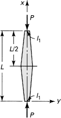
where I1 is the constant moment of inertia at x = 0 and x = L.
Solution
As before, we begin by representing the deflection by
![]()
Taking symmetry into account, the variation of strain energy and the work done [Eqs. (11.21) and (11.22)] are expressed by
![]()
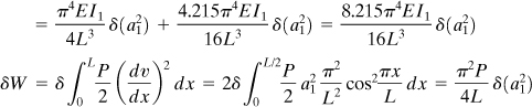
From the principle of virtual work, δW = δU, we have
![]()
or
![]()
In Example 11.8, this problem is solved by numerical analysis, revealing that the preceding solution overestimates the buckling load.
Example 11.6. Critical Load of a Rail on a Track
Consider the beam of Fig. 11.15, representing a rail on a track experiencing compression owing to a rise in temperature. Determine the critical load.
Figure 11.15. Example 11.6. Beam with hinged ends, embedded in an elastic foundation of modulus k, subjected to compressive end forces.

Solution
We choose the deflection shape in the form of a series given by Eq. (10.23). The solution proceeds as in Example 10.13. Now the total energy consists of three sources: beam bending and compression and foundation displacement. The strain energy in bending, from Eq. (10.25), is
![]()
The strain energy due to the deformation of the elastic foundation is given by Eq. (10.30):
![]()
The work done by the forces P in shortening the span, using Eq. (10.31), is
![]()
Applying the principle of virtual work, δW = δ(U1 + U2), we obtain
![]()
The foregoing results in the critical load:
(11.28)
Note that this expression yields exact results. The lowest critical load may occur with n = 1, 2, 3, ..., depending on the properties of the beam and the foundation [Ref. 11.1].
Interestingly, taking n = 1, Eq. (11.28) becomes
(m)
which is substantially greater than the Euler load. The Euler buckling load is the first term; it is augmented by kL2/π2 due to the foundation.
11.11 Solution by Finite Differences
The equilibrium analysis of buckling often leads to differential equations that resist solution. Even energy methods are limited in that they require that the moment of inertia be expressible as a function of the column length coordinate. Therefore, to enable the analyst to cope with the numerous and varied columns of practical interest, numerical techniques must be relied on. The examples that follow apply the method of finite differences to the differential equation of a column.
Example 11.7. Analysis of a Simple Column
Determine the buckling load of a pin-ended column of length L and constant cross section. Use four subdivisions of equal length. Denote the nodal points by 0, 1, 2, 3, and 4, with 0 and 4 located at the ends. Locate the origin of coordinates at the stationary end.
Solution
The governing differential equation (11.1) may be put into the form
![]()
by substituting λ2 = P/EI. The boundary conditions are v(0) = v(L) = 0. The corresponding finite difference equation is, according to Eq. (7.9),
(11.29)
valid at every node along the length. Here the integer m denotes the nodal points, and h the segment length. Applying Eq. (11.29) at points 1, 2, and 3, we have

(a)
or, in convenient matrix form,
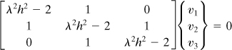
(b)
This set of simultaneous equations has a nontrivial solution for v1, v2, and v3 only if the determinant of the coefficients vanishes:

(c)
The solution of the buckling problem is thus reduced to determination of the roots (the λ’s of the characteristic equation) resulting from the expansion of the determinant.
To expedite the solution, we take into account the symmetry of deflection. For the lowest critical load, the buckling configuration is given by the first mode, shown in Fig. 11.3a. Thus, v1 = v3, and the Eqs. (a) become
(λ2h2 – 2)v1 + v2 = 0
2v1 + (λ2h2 – 2)v2 = 0
Setting equal to zero the characteristic determinant of this set, we find that (λ2h2 – 2)2 – 2 = 0, which has the solution ![]() . Selecting
. Selecting ![]() to obtain a minimum critical value and letting h = L/4, we obtain
to obtain a minimum critical value and letting h = L/4, we obtain ![]() . Thus,
. Thus,
![]()
This result differs from the exact solution by approximately 5%. By increasing the number of segments, the accuracy may be improved.
If required, the critical load corresponding to second-mode buckling, indicated in Fig. 11.3b, may be determined by recognizing that for this case v0 = v2 = v4 = 0 and v1 = –v3. We then proceed from Eqs. (a) as before. For buckling of higher than second mode, a similar procedure is followed, in which the number of segments is increased and the appropriate conditions of symmetry satisfied.
Example 11.8. Critical Load of a Tapered Column
What load will cause buckling of the tapered pin-ended column shown in Fig. 11.14?
Solution
The finite difference equation is given by Eq. (11.29):
(d)
The foregoing becomes, after substitution of I(x),
(e)
where λ2 = P/EI1. Note that the coefficient of vm is a variable, dependent on x. This introduces no additional difficulties, however.
Dividing the beam into two segments, we have h = L/2 (Fig. 11.16a). Applying Eq. (e) at x = L/2,
![]()
Figure 11.16. Example 11.8. Division of the column of Fig. 11.14 into a number of segments.
The nontrivial solution corresponds to v1 ≠ 0; then (λ2L2/10) – 2 = 0 or, by letting λ2 = P/EI,
(f)
Similarly, for three segments h = L/3 (Fig. 11.16b). From symmetry, we have v1 = v2, and v0 = v3 = 0. Thus, Eq. (e) applied at x = L/3 yields
![]()
(g)
For h = L/4, referring to Fig. 11.16c, Eq. (e) leads to
![]()
For a nontrivial solution, the characteristic determinant is zero:
![]()
Expansion yields
λ4L4 – 136λ2L2 + 2240 = 0
for which
(h)
Similar procedures considering the symmetry shown in Figs. 11.16d and e lead to the following results:
For h = L/5,
(i)
For h = L/6,
(j)
Results (f) through (j) indicate that, for columns of variable moment of inertia, increasing the number of segments does not necessarily lead to improved Pcr. An energy approach to this problem (Example 11.5) gives the result Pcr = 20.25EI1/L2. Because this value is higher than those obtained here, we conclude that the column does not deflect into the half sine curve assumed in Example 11.5.
Example 11.9. Critical Load of a Fixed-Pinned Column
Figure 11.17 shows a column of constant moment of inertia I and of length L, fixed at the left end and simply supported at the right end, subjected to an axial compressive load P. Determine the critical value of P using m = 3.
Figure 11.17. Example 11.9. Fixed-Pinned column.
Solution
The characteristic value problem is defined by
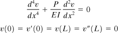
(k)
where the first equation is found from Eq. (P11.34) by setting p = 0; the second expression represents the end conditions related to deflection, slope, and moment. Equations (k), referring to Section 7.2 and letting λ2 = P/EI, may be written in the finite difference form as follows:
(l)
and
(m)
The quantities v–1 and vm + 1 represent the deflections at the nodal points of the column prolonged by h beyond the supports. By dividing the column into three subintervals, the pattern of the deflection curve and the conditions (m) are represented in the figure by dashed lines. Now, Eq. (l) is applied at nodes 1 and 2 to yield, respectively,
v1 + (6 – 2λ2h2)v1 + (λ2h2 – 4)v2 = 0
(λ2h2 – 4)v1 + (6 – 2λ2h2)v2 – v2 = 0
We have a nonzero solution if the determinant of the coefficients of these equations vanishes:
![]()
From this and setting h = L/3, we obtain λ2 = 16.063/L. Thus,
(n)
The exact solution is 20.187EI/L2. By increasing the number of segments and by employing an extrapolation technique, the results may be improved.
11.12 Finite Difference Solution for Unevenly Spaced Nodes
It is often advantageous, primarily because of geometrical considerations, to divide a structural element so as to produce uneven spacing between nodal points. In some problems, uneven spacing provides more than a saving in time and effort. As seen in Section 7.4, some situations cannot be solved without resort to this approach.
Consider the problem of the buckling of a straight pin-ended column governed by
![]()
Upon substitution from Eq. (7.21), the following corresponding finite difference equation is obtained:
(11.30)
where
(11.31)
Equation (11.30), valid throughout the length of the column, is illustrated in the example to follow.
Example 11.10. Critical Load of a Stepped Column
Determine the buckling load of a stepped pin-ended column (Fig. 11.18a). The variation of the moment of inertia is indicated in the figure.
Figure 11.18. Example 11.10. Stepped column with pinned ends.

Solution
The nodal points are shown in Fig. 11.18b and are numbered in a manner consistent with the symmetry of the beam. Note that the nodes are unevenly spaced. From Eq. (11.31), we have α1 = 2 and α2 = 1. Application of Eq. (11.30) at points 1 and 2 leads to
![]()
![]()
or

For a nontrivial solution, it is required that
![]()
Solving, we find that the root corresponding to minimum P is
![]()
Employing additional nodal points may result in greater accuracy. This procedure lends itself to columns of arbitrarily varying section and various end conditions.
We conclude our discussion by noting that column buckling represents but one case of structural instability. Other examples include the lateral buckling of a narrow beam; the buckling of a flat plate compressed in its plane; the buckling of a circular ring subject to radial compression; the buckling of a cylinder loaded by torsion, compression, bending, or internal pressure; and the snap buckling of arches. Buckling analyses for these cases are often not performed as readily as in the examples presented in this chapter. The solutions more often involve considerable difficulty and subtlety.*
References
11.1. TIMOSHENKO, S. P., and GERE, J. M., Theory of Elastic Stability, 3rd ed., McGraw-Hill, New York, 1970, Secs. 2.7 and 2.10.
11.2. SHANLEY, R. F., Mechanics of Materials, McGraw-Hill, New York, 1967, Sec. 11.3.
11.3. PEERY, D. J., and AZAR, J. J., Aircraft Structures, 2nd ed., McGraw-Hill, New York, 1993, Chap.12.
11.4. UGURAL, A. C., Mechanical Design: An Integrated Approach, McGraw-Hill, New York, 2004.
11.5. Manual of Steel Construction, latest ed., American Institute of Steel Construction, Inc., Chicago.
11.6. UGURAL, A. C., Mechanics of Materials, Wiley, Hoboken, N. J., 2008, Sec. 11.7.
11.7. TIMOSHENKO, S. P., and GERE, J. M., Theory of Elastic Stability, 3rd ed., McGraw-Hill, New York, 1970, Chaps. 2 through 6.
11.8. BORESI, A. P., and SCHMIDTH, R. J., Advanced Mechanics of Materials, 6th ed., Wiley, Hoboken, N.J., 2003.
11.9. UGURAL, A. C., Stresses in Beams, Plates, and Shells, 3rd ed., CRC Press, Taylor and Francis Group, Boca Raton, Fla., 2010.
11.10. BRUSH, D. O., and ALMROTH, B. O., Buckling of Bars, Plates, and Shells, McGraw-Hill, New York, 1975.
Problems
Sections 11.1 through 11.7
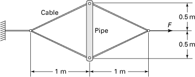
11.1. In the assembly shown in Figure P11.1, a 50-mm outer-diameter and 40-mm inner-diameter steel pipe (E = 200 GPa) that is 1-m long acts as a spreader member. For a factor of safety n = 2.5, what is the value of F that will cause buckling of the pipe?
11.2. Figure P11.2 shows the cross sections of two aluminum alloy 2114-T6 bars that are used as compression members, each with effective length of Le. Find (a) the wall thickness the hollow square bar so that the bars have the same cross-sectional area; (b) the critical load of each bar. Given: Le = 3 m and E = 72 GPa (from Table D.1).

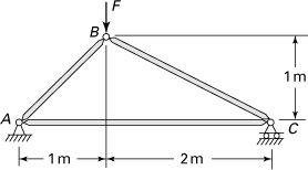
11.3. Based on a factor of safety n = 1.8, determine the maximum load F that can be applied to the truss shown in Figs. P11.3. Given: Each column is of 50-mm-diameter aluminum bar having E = 70 GPa.
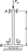
11.4. Figure P11.4 shows a column AB of length L and flexural rigidity EI with a support at its base that does not permit rotation but allows horizontal displacement and is pinned at its top. What is the critical load Pcr?
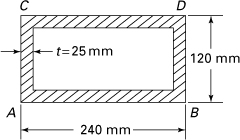
11.5. Figure P11.5 shows the tube of uniform thickness t = 25 mm cross section of a fixed-ended rectangular steel (E = 200 GPa) of a 9-m-long column. Determine the critical stress in the column.
11.6. Resolve Prob. 11.5 for the case in which the column is pinned at one end and fixed at the other.
11.7. Brace BD of the structure illustrated in Fig. P11.7 is made of a steel rod (E = 210 GPa and σyp = 250 MPa) with a square cross section (50 mm on a side). Calculate the factor of safety n against failure by buckling.

11.8. Verify the specific Johnson’s formulas, given by Eqs. (11.11) and (11.12), for the intermediate sizes of columns with solid circular and rectangular cross sections, respectively.
11.9. A steel column with pinned ends supports an axial load P = 90 kN. Calculate the longest allowable column length. Given: Cross-sectional area A = 3 × 103 mm2 and radius of gyration r = 25 mm; the material properties are E = 200 GPa and σyp = 250 MPa.
11.10. Compute the allowable axial load P for a wide-flange steel column with fixed-fixed ends and a length of 12 m, braced at midpoint C (Fig. P11.10). Given: Material properties E = 210 GPa, σyp = 280 MPa; cross-sectional area A = 27 × 103 mm2 and radius of gyration r = 100 mm.

Sections 11.1 through 11.7
11.11. A column of length 3L is approximated by three bars of equal length connected by a torsional spring of appropriate stiffness k at each joint. The column is supported by a torsional spring of stiffness k at one end and is free at the other end. Derive an expression for determining the critical load of the system. Generalize the problem to the case of n connected bars.
11.12. A 3-m-long fixed-ended column (Le = 1.5 m) is made of a solid bronze rod (E = 110 GPa) of diameter D = 30 mm. To reduce the weight of the column by 25%, the solid rod is replaced by the hollow rod of cross section shown in Fig. P11.12. Compute (a) the percentage of reduction in the critical load and (b) the critical load for the hollow rod.

11.13. A 2-m-long pin-ended column of square cross section is to be constructed of timber for which E = 11 GPa and σall = 15 MPa for compression parallel to the grain. Using a factor of safety of 2 in computing Euler’s buckling load, determine the size of the cross section if the column is to safely support (a) a 100-kN load and (b) a 200-kN load.
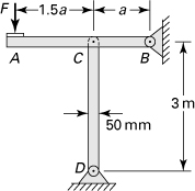
11.14. A horizontal rigid bar AB is supported by a pin-ended column CD and carries a load F (Fig. P11.14). The column is made of steel bar having 50- by 50-mm square cross section, 3 m length, and E = 200 GPa. What is the allowable value of F based a factor of safety of n = 2.2 with respect to buckling of the column?
11.15. A uniform steel column, with fixed- and hinge-connected ends, is subjected to a vertical load P = 450 kN. The cross section of the column is 0.05 by 0.075 m and the length is 3.6 m. Taking σyp = 280 MPa and E = 210 GPa, calculate (a) the critical load and critical Euler stress, assuming a factor of safety of 2, and (b) the allowable stress according to the AISC formula, Eq. (11.13).
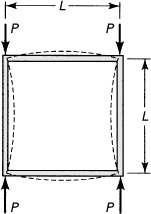
11.16. Figure P11.16 shows a square frame. Determine the critical value of the compressive forces P. All members are of equal length L and of equal modulus of rigidity EI. Assume that symmetrical buckling, indicated by the dashed lines in the figure, occurs.
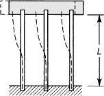
11.17. A rigid block of weight W is to be supported by three identical steel bars. The bars are fixed at each end (Fig. P11.17). Assume that sidesway is not prevented and that, when an additional downward force of 2W is applied at the middle of the block, buckling will take place as indicated by the dashed lines in the figure. Find the effective lengths of the columns by solving the differential equation for deflection of the column axis.
11.18. A simply supported beam of flexural rigidity EIb is propped up at its center by a column of flexural rigidity EIc (Fig. P11.18). Determine the midspan deflection of the beam if it is subjected to a uniform load p per unit length.

11.19. Two in-line identical cantilevers of cross-sectional area A, rigidity EI, and coefficient of thermal expansion α are separated by a small gap δ. What temperature rise will cause the beams to (a) just touch and (b) buckle elastically?
11.20. A W203 × 25 column fixed at both ends has a minimum radius of gyration r = 29.4 mm, cross-sectional area A = 3230 mm2, and length 1.94 m. It is made of a material whose compression stress–strain diagram is given in Fig. P11.20 by dashed lines. Find the critical load. The stress–strain diagram may be approximated by a series of tangentlike segments, the accuracy improving as the number of segments increases. For simplicity, use four segments, as indicated in the figure. The modulus of elasticity and various tangent moduli (the slopes) are labeled.

11.21. The pin-jointed structure shown in Fig. P11.21 is constructed of two 0.025-m-diameter tubes having the following properties: A = 5.4 × 10⁻⁵ m2, I = 3.91 × 10⁻⁹ m4, E = 210 GPa. The stress–strain curve for the tube material can be accurately approximated by three straight lines as shown. If the load P is increased until the structure fails, which tube fails first? Describe the nature of the failure and determine the critical load.

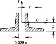
11.22. Two 0.075- by 0.075-m equal leg angles, positioned with the legs 0.025 m apart back to back, as shown in Fig. P11.22, are used as a column. The angles are made of structural steel with σyp = 203 MPa and E = 210 GPa. The area properties of an angle are thickness t = 0.0125 m, A = 1.719 × 10⁻³ m2, Ic = 8.6 × 10⁻⁷m4, I/c = S = 1.719 × 10⁻⁵ m3, rc = 0.0225 m, and ![]() =
= ![]() = 0.02325 m. Assume that the columns are connected by lacing bars that cause them to act as a unit. Determine the critical stress of the column by using the AISC formula, Eq. (11.13), for effective column lengths (a) 2.1 m and (b) 4.2 m.
= 0.02325 m. Assume that the columns are connected by lacing bars that cause them to act as a unit. Determine the critical stress of the column by using the AISC formula, Eq. (11.13), for effective column lengths (a) 2.1 m and (b) 4.2 m.
11.23. Redo Prob. 11.22(b) using the Euler formula.
11.24. A 1.2-m-long, 0.025- by 0.05-m rectangular column with rounded ends fits perfectly between a rigid ceiling and a rigid floor. Compute the change in temperature that will cause the column to buckle. Let α = 10 × 10–6/°C, E = 140 GPa, and σyp = 280 MPa.
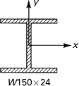
11.25. A pin-ended W150 × 24 rolled-steel column of cross section shown in Fig. P11.25 (A = 3.06 × 103 mm2, rx = 66 mm, and ry = 24.6 mm) carries an axial load of 125 kN. What is the longest allowable column length according to the AISC formula? Use E = 200 GPa and σyp = 250 Pa.
Sections 11.8 and 11.9
11.26. A pinned-end rod AB of diameter d supports an eccentrically applied load of P, as depicted in Fig. P11.26. Assuming that the maximum deflection at the midlength is vmax, determine (a) the eccentricity e; (b) the maximum stress in the rod. Given: d = 40 mm, P = 80 kN, vmax = 1.0 mm, and E = 200 GPa.

11.27. Redo Prob. 11.26 for the case in which column AB is fixed at base B and free at top A.
11.28. A cast-iron hollow-box column of length L is fixed at its base and free at its top, as depicted in Fig. P11.28. Assuming that an eccentric load P acts at the middle of side AB (that is, e = 50 mm) of the free end, determine the maximum stress σmax in the column. Given: P = 250 kN, L = 1.8 m, E = 70 GPa, and e = 50 mm.
11.29. Resolve Prob. 11.28, knowing that the load acts at the middle of side AC (that is, e = 100 mm).
11.30. A steel bar (E = 210 GPa) of b = 50 mm by h = 25 mm rectangular cross section (Fig. P11.30) and length L = 1.5 m is eccentrically compressed by axial loads P = 10 kN. The forces are applied at the middle of the long edge of the cross section. What are the maximum deflection vmax and maximum bending moment Mmax?
11.31. A 0.05-m square, horizontal steel bar, 9-m long, is simply supported at each end. The only force acting is the weight of the bar. (a) Find the maximum stress and deflection. (b) Assume that an axial compressive load of 4.5 kN is also applied at each end through the centroid of cross-sectional area. Determine the stress and deflection under this combined loading. For steel, the specific weight is 77 kN/m3, E = 210 GPa, and v = 0.3.
11.32. The properties of a W203 × 46 steel link are A = 5880 mm2, Iz ≈ 45.66 × 106 mm4, Iy ≈ 15.4 × 106 mm4, depth = 203.2 mm, width of flange = 203.2 mm, and E = 210 GPa. What maximum end load P can be applied at both ends, given an eccentricity of 0.05 m along axis yy? A stress of 210 MPa is not to be exceeded. Assume that the effective column length of the link is 4.5 m.
11.33. A hinge-ended bar of length L and stiffness EI has an initial curvature expressed by v0 = a1 sin(πx/L) + 5a1 sin(2πx/L). If this bar is subjected to an increasing axial load P, what value of the load P, expressed in terms of L, E, and I, will result in zero deflection at x = 3L/4?
11.34. Employing the equilibrium approach, derive the following differential equation for a simply supported beam column subjected to an arbitrary distributed transverse loading p(x) and axial force P:
(P11.34)
Demonstrate that the homogeneous solution for this equation is
![]()
where the four constants of integration will require, for evaluation, four boundary conditions.
Section 11.10
11.35. Assuming v = a0[1 – (2x/L)2], determine the buckling load of a pin-ended column. Employ the Rayleigh–Ritz method, placing the origin at midspan.
11.36. The cross section of a pin-ended column varies as in Fig. P11.36. Determine the critical load using an energy approach.

11.37. A cantilever column has a moment of inertia varying as I = I1(1 – x/2L), where I1 is the constant moment of inertia at the fixed end (x = 0). Find the buckling load by choosing v = v1(x/L)2. Here v1 is the deflection of the free end.
11.38. Derive an expression for the deflection of the uniform pin-ended beam-column of length L, subjected to a uniform transverse load p and axial compressive force P. Use an energy approach.
11.39. A simply supported beam column of length L is subjected to compression forces P at both ends and lateral loads F and 2F at quarter-length and midlength, respectively. Employ the Rayleigh–Ritz method to determine the beam deflection.
11.40. Determine the critical compressive load P that can be carried by a cantilever at its free end (x = L). Use the Rayleigh–Ritz method and let v = x2(L – x)(a + bx), where a and b are constants.
Sections 11.11 and 11.12
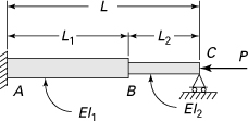
11.41. A stepped cantilever beam with a hinged end, subjected to the axial compressive load P, is shown in Fig. P11.41. Determine the critical value of P, applying the method of finite differences. Let m = 3 and L1 = L2 = L/2.
11.42. A uniform cantilever column is subjected to axial compression at the free end (x = L). Determine the critical load. Employ the finite differences, using m = 2. [Hint: The boundary conditions are v(0) = v′(0) = v″(L) = v″′(L) = 0.]
11.43. The cross section of a pin-ended column varies as in Fig. P11.36. Determine the critical load using the method of finite differences. Let m = 4.
11.44. Find the critical value of the load P in Fig. P11.41 if both ends of the beam are simply supported. Let L1 = L/4 and L2 = 3L/4. Employ the method of finite differences by taking the nodes at x = 0, x = L/4, x = L/2, and x = L.