
Chapter 12. Plastic Behavior of Materials
12.1 Introduction
Thus far, we have considered loadings that cause the material of a member to behave elastically. We are now concern with the behavior of machine and structural components when stresses exceed the proportional limit. In such cases it is necessary to make use of the stress–strain diagrams obtained from an actual test of the material, or an idealized stress–strain diagram. For purposes of analysis, a single mathematical expression will often be employed for the entire stress–strain diagram. Deformations and stresses in members made of elastic–plastic and rigid-plastic materials having various forms will be determined under single and combined loadings. Applications include collapse load of structures, limit design, membrane analogy, rotating disks, and pressure vessels.
The plasticity describes the inelastic behavior of a material that retains permanent yielding on complete unloading. The subject of plasticity is perhaps best introduced by recalling the principal characteristics of elastic behavior. First, a material subjected to stressing within the elastic regime will return to its original state upon removal of those external influences causing application of load or displacement. Second, the deformation corresponding to a given stress depends solely on that stress and not on the history of strain or load. In plastic behavior, opposite characteristics are observed. The permanent distortion that takes place in the plastic range of a material can assume considerable proportions. This distortion depends not only on the final state of stress but on the stress states existing from the start of the loading process as well.
The equations of equilibrium (1.14), the conditions of compatibility (2.12), and the strain–displacement relationships (2.4) are all valid in plastic theory. New relationships must, however, be derived to connect stress and strain. The various yield criteria (discussed in Chap. 4), which strictly speaking are not required in solving a problem in elasticity, play a direct and important role in plasticity. This chapter can provide only an introduction to what is an active area of contemporary design and research in the mechanics of solids.* The basics presented can, however, indicate the potential of the field, as well as its complexities.
12.2 Plastic Deformation
We shall here deal with the permanent alteration in the shape of a polycrystalline solid subject to external loading. The crystals are assumed to be randomly oriented. As has been demonstrated in Section 2.15, the stresses acting on an elemental cube can be resolved into those associated with change of volume (dilatation) and those causing distortion or change of shape. The distortional stresses are usually referred to as the deviator stresses.
The dilatational stresses, such as hydrostatic pressures, can clearly decrease the volume while they are applied. The volume change is recoverable, however, upon removal of external load. This is because the material cannot be compelled to assume, in the absence of external loading, interatomic distances different from the initial values. When the dilatational stresses are removed, therefore, the atoms revert to their original position. Under the conditions described, no plastic behavior is noted, and the volume is essentially unchanged upon removal of load.
In contrast with the situation described, during change of shape, the atoms within a crystal of a polycrystalline solid slide over one another. This slip action, referred to as dislocation, is a complex phenomenon. Dislocation can occur only by the shearing of atomic layers, and consequently it is primarily the shear component of the deviator stresses that controls plastic deformation. Experimental evidence supports the assumption that associated with plastic deformation essentially no volume change occurs; that is, the material is incompressible (Sec. 2.10):
(12.1)
Therefore, from Eq. (2.39), Poisson’s ratio ![]() for a plastic material.
for a plastic material.
Slip begins at an imperfection in the lattice, for example, along a plane separating two regions, one having one more atom per row than the other. Because slip does not occur simultaneously along every atomic plane, the deformation appears discontinuous on the microscopic level of the crystal grains. The overall effect, however, is plastic shear along certain slip planes, and the behavior described is approximately that of the ideal plastic solid. As the deformation continues, a locking of the dislocations takes place, resulting in strain hardening or cold working.
In performing engineering analyses of stresses in the plastic range, we do not usually need to consider dislocation theory, and the explanation offered previously, while overly simple, will suffice. What is of great importance to the analyst, however, is the experimentally determined curves of stress and strain.
12.3 Idealized Stress–Strain Diagrams
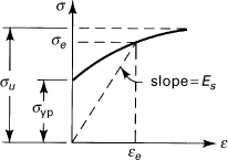
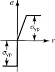
The bulk of present-day analysis in plasticity is predicated on materials displaying idealized stress–strain curves as in Fig. 12.1a and c. Such materials are referred to as rigid, perfectly plastic and elastic-perfectly plastic, respectively. Examples include mild steel, clay, and nylon, which exhibit negligible elastic strains in comparison with large plastic deformations at practically constant stress. A more realistic portrayal including strain hardening is given in Fig. 12.1b for what is called a rigid-plastic solid. In the curves, a and b designate the tensile yield and ultimate stresses, σyp and σu, respectively. The curves of Fig. 12.1c and d do not ignore the elastic strain, which must be included in a more general stress–strain depiction. The latter figures thus represent idealized elastic–plastic diagrams for the perfectly plastic and plastic materials, respectively. The material in Figs. 12.c and d is also called a strain-hardening or work-hardening material. For a linearly strain-hardening material, the regions ab of the diagrams become a sloped straight line.
Figure 12.1. Idealized stress–strain diagrams: (a) rigid, perfectly plastic material; (b) rigid-plastic material; (c) elastic, perfectly plastic material; and (d) elastic, rigid-plastic material.

True Stress–True Strain Relationships
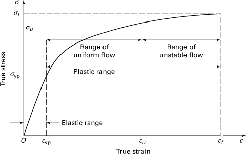
Consider the idealized true stress–strain diagram given in Fig. 12.2. The fracture stress and fracture strain are denoted by σf and εf, respectively. The fundamental design utility of the plot ends at the ultimate stress σu. Note that a comparison of a true and nominal σ – ε plot is shown in Fig. 2.12. In addition to the preceding idealized cases, various theoretical analyses have been advanced to predict plastic behavior. Equations relating stress and strain beyond the proportional limit range from the rather empirical to those leading to complex mathematical approaches applicable to materials of specific type and structure. For purposes of an accurate analysis, a single mathematical expression is frequently employed for the entire stress–strain curve. An equation representing the range of σ – ε diagrams, especially useful for aluminum and magnesium, has been developed by Ramberg and Osgood [Ref. 12.4]. We confine our discussion to that of a perfectly plastic material displaying a horizontal straight-line relationship and to the parabolic relationship described next.
Figure 12.2. Idealized true stress–strain diagram.
For many materials, the entire true stress–true strain curve may be represented by the parabolic form
(12.2)
where n and K are the strain-hardening index and the strength coefficient, respectively. The definitions of true stress and true strain are given in Section 2.7. The curves of Eq. (12.2) are shown in Fig. 12.3a. We observe from the figure that the slope dσ/dε grows without limit as ε approaches zero for n ≠ 1. Thus, Eq. (12.2) should not be used for small strains when n ≠ 1. The stress–strain diagram of a perfectly plastic material is represented by this equation when n = 0 (and hence K = σyp). Clearly, for elastic materials (n = 1 and hence K = E), Eq. (12.2) represents Hooke’s law, wherein E is the modulus of elasticity.
Figure 12.3. (a) Graphical representation of σ = Kεn; (b) true stress versus true strain on log–log coordinates.

For a particular material, with true stress–true strain data available, K and n are readily evaluated inasmuch as Eq. (12.2) plots as a straight line on logarithmic coordinates. We can thus rewrite Eq. (12.2) in the form
(a)
Here n is the slope of the line and K the true stress associated with the true strain at 1.0 on the log–log plot (Fig. 12.3b). The strain-hardening coefficient n for commercially used materials falls between 0.2 and 0.5. Fortunately, with the use of computers, much refined modeling of the stress–strain relations for real material is possible.
12.4 Instability in Simple Tension
We now describe an instability phenomenon in uniaxial tension of practical importance in predicting the maximum allowable plastic stress in a rigid-plastic material. At the ultimate stress σu in a tensile test (Fig. 12.2), an unstable flow results from the effects of strain hardening and the decreasing cross-sectional area of the specimen. These tend to weaken the material. When the rate of the former effect is less than the latter, an instability occurs. This point corresponds to the maximum tensile load and is defined by
(a)
Since axial load P is a function of both the true stress and the area (P = σA), Eq. (a) is rewritten
(b)
The condition of incompressibility, Ao Lo = AL, also yields
(c)
as the original volume Ao Lo is constant. Expressions (b) and (c) result in
(d)
From Eqs. (2.25) and (d), we thus obtain the relationships
(12.3)
for the instability of a tensile member. Here the subscript o denotes the engineering strain and stress (Sec. 2.7).
Introduction of Eq. (12.2) into Eq. (12.3) results in
![]()
or
(12.4)
That is, at the instant of instability of flow in tension, the true strain ε has the same numerical value as the strain-hardening index. The state of true stress and the true strain under uniaxial tension are therefore
(e)
The problem of instability under simple compression or plastic buckling is discussed in Section 11.6. The instability condition for cases involving biaxial tension is derived in Sections 12.12 and 12.13.
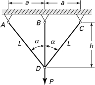
Example 12.1. Three-Bar Structure
Determine the maximum allowable plastic stress and strain in the pin-jointed structure sustaining a vertical load P, shown in Fig. 12.4. Assume that α = 45° and that each element is constructed of an aluminum alloy with the following properties:
σyp = 350 MPa, K = 840 MPa, n = 0.2
AAD = ACD = 10 × 10–5 m2, ABD = 15 × 10–5 m2, h = 3 m
Figure 12.4. Example 12.1. Pin-connected structure in axial tension.
Solution
The structure is elastically statically indeterminate, and the solution may readily be obtained on applying Castigliano’s theorem (Sec. 10.7). Plastic yielding begins upon loading:
![]()
On applying Eqs. (e), the maximum allowable stress
σ = Knn = 840 × 106(0.2)0.2 = 608.9 MPa
occurs at the following axial and transverse strains:
ε1 = n = 0.2, ε2 = ε3 = –0.1
We have L = h/cos α. The total elongations for instability of the bars are thus δBD = 3(0.2) = 0.6 m and δAB = δCD = (3/cos 45°)(0.2) = 0.85 m.
Example 12.2. Tube in Axial Tension
A tube of original mean diameter do and thickness to is subjected to axial tensile loading. Assume a true stress–engineering strain relation of the form ![]() and derive expressions for the thickness and diameter at the instant of instability. Let n = 0.3.
and derive expressions for the thickness and diameter at the instant of instability. Let n = 0.3.
Solution
Differentiating the given expression for stress,
![]()
This result and Eq. (12.3) yield the engineering axial strain at instability:
(f)
The transverse strains are –εo/2, and hence the decrease of wall thickness equals nto/2(1 – n). The thickness at instability is thus
(g)
Similarly, the diameter at instability is
(h)
From Eqs. (g) and (h), with n = 0.3, we have t = 0.79to and d = 0.79do. Thus, for the tube under axial tension, the diameter and thickness decrease approximately 21% at the instant of instability.
12.5 Plastic Axial Deformation and Residual Stress
As pointed out earlier, if the stress in any part of the member exceeds the yield strength of the material, plastic deformations occur. The stress that remains in a structural member upon removal of external loads is referred to as the residual stress. The presence of residual stress may be very harmful or, if properly controlled, may result in substantial benefit.
Plastic behavior of ductile materials may be conveniently represented by considering an idealized elastoplastic material shown in Fig. 12.5, where σyp and εyp designate the yield strength and yield strain, respectively. The Y corresponds to the onset of yield in the material. The part OB is the strain corresponding to the plastic deformation that results from the loading and unloading of the specimen along line AB parallel to the initial portion OY of the loading curve.
Figure 12.5. Tensile stress–strain diagram for elastoplastic material.

The distribution of residual stresses can be found by superposition of the stresses owing to loading and the reverse, or rebound, stresses due to unloading. (The strains corresponding to the latter are the reverse, or rebound, strains.) The reverse stress pattern is assumed to be fully elastic and consequently can be obtained applying Hooke’s law. That means the linear relationship between σ and ε remains valid, as illustrated by line AB in the figure. We note that this superposition approach is not valid if the residual stresses thereby found exceed the yield strength.
The nonuniform deformations that may be caused in a material by plastic bending and plastic torsion are considered in Sections 12.7 and 12.9. This section is concerned with a restrained or statically indeterminate structure that is axially loaded beyond the elastic range. For such a case, some members of the structure experience different plastic deformation, and these members retain stress following the release of load.
The magnitude of the axial load at the onset of yielding, or yield load Pyp, in a statically determinate ductile bar of cross-sectional area A is σyp A. This also is equal to the plastic, limit, or ultimate load Pu of the bar. For a statically indeterminate structure, however, after one member yields, additional load is applied until the remaining members also reach their yield limits. At this time, unrestricted or uncontained plastic flow occurs, and the limit load Pu is reached. Therefore, the ultimate load is the load at which yielding begins in all materials.
Examples 12.3, 12.7, and 12.12 illustrate how plastic deformations and residual stresses are produced and how the limit load is determined in axially loaded members, beams, and torsional members, respectively.
Example 12.3. Residual Stresses in an Assembly
Figure 12.6a shows a steel bar of 750-mm2 cross-sectional area placed between two aluminum bars, each of 500-mm2 cross-sectional area. The ends of the bars are attached to a rigid support on one side and a rigid thick plate on the other. Given: Es = 210 GPa, (σs)yp = 240 MPa, Ea = 70 GPa, and (σa)yp = 320 MPa. Assumption: The material is elastic–plastic.
Figure 12.6. Example 12.3. (a) Plastic analysis of a statically indeterminate three-bar structure; (b) free-body diagram of end plate.
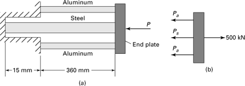
Calculate the residual stress, for the case in which applied load P is increased from zero to Pu and removed.
Solution
Material Behavior. At ultimate load Pu both materials yield. Either material yielding by itself will not result in failure because the other material is still in the elastic range. We therefore have
Pa = 500(320) = 160 kN, Ps = 750(240) = 180 kN
Hence,
Pu = 2(160) + 180 = 500 kN
Applying an equal and opposite load of this amount, equivalent to a release load (Fig. 12.6b), causes each bar to rebound elastically.
Geometry of Deformation. Condition of geometric fit, δa = δs gives
(a)
Condition of Equilibrium. From the free-body diagram of Fig. 12.6b,
(b)
Solving Eqs. (a) and (b) we obtain
![]()
Superposition of the initial forces at ultimate load Pu and the elastic rebound forces owing to release of Pu results in:
(Pa)res = 79.1 – 160 = –80.9 kN
(Ps)res = 341.7 – 180 = 161.7 kN
The associated residual stresses are thus
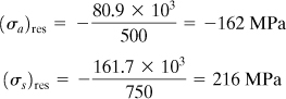
Comment
We note that after this prestressing process, the assembly remains elastic as long as the value of Pu = 500 kN is not exceeded.
12.6 Plastic Deflection of Beams
In this section we treat the inelastic deflection of a beam, employing the mechanics of materials approach. Consider a beam of rectangular section, as in Fig. 12.7a, wherein the bending moment M produces a radius of curvature r. The longitudinal strain of any fiber located a distance y from the neutral surface, from Eq. (5.9), is given by
Figure 12.7. (a) Inelastic bending of a rectangular beam in pure bending; (b) stress–strain diagram for an elastic-rigid plastic material.
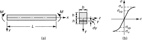
(12.5)
Assume the beam material to possess equal properties in tension and compression. Then, the longitudinal tensile and compressive forces cancel, and the equilibrium of axial forces is satisfied. The following describes the equilibrium of moments about the z axis (Fig. 12.7a):
(a)
For any specific distribution of stress, as, for example, that shown in Fig. 12.7b, Eq. (a) provides M and then the deflection, as is demonstrated next.
Consider the true stress–true strain relationship of the form σ = Kεn. Introducing this together with Eq. (12.5) into Eq. (a), we obtain
(b)
where
(12.6)
From Eqs. (12.5), σ = Kεn, and (b) the following is derived:
(c)
In addition, on the basis of the elementary beam theory, we have, from Eq. (5.7),
(d)
Upon substituting Eq. (c) into Eq. (d), we obtain the following equation for a rigid plastic beam:
(12.7)
It is noted that when n = 1 (and hence K = E), this expression, as expected, reduces to that of an elastic beam [Eq. (5.10)].
Example 12.4. Rigid-Plastic Simple Beam
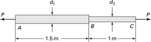
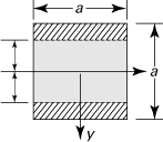
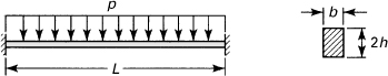
Determine the deflection of a rigid-plastic simply supported beam subjected to a downward concentrated force P at its midlength. The beam has a rectangular cross section of depth 2h and width b (Fig. 12.8).
Figure 12.8. Examples 12.4 and 12.8.
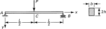
Solution
The bending moment for segment AC is given by
(e)
where the minus sign is due to the sign convention of Section 5.2.
Substituting Eq. (e) into Eq. (12.7) and integrating, we have

(f)
where
(g)
The constants of integration c1 and c2 depend on the boundary conditions v(0) = dv/dx(L/2) = 0:
![]()
Upon introduction of c1 and c2 into Eq. (f), the beam deflection is found to be
(12.8)
Interestingly, in the case of an elastic beam, this becomes
![]()
For x = L/2, the familiar result is
![]()
The foregoing procedure is applicable to the determination of the deflection of beams subject to a variety of end conditions and load configurations. It is clear, however, that owing to the nonlinearity of the stress law, σ = Kεn, the principle of superposition cannot validly be applied.
12.7 Analysis of Perfectly Plastic Beams
By neglecting strain hardening, that is, by assuming a perfectly plastic material, considerable simplification can be realized. We shall, in this section, focus our attention on the analysis of a perfectly plastic straight beam of rectangular section subject to pure bending (Fig. 12.7a).
The bending moment at which plastic deformation impends, Myp, may be found directly from the flexure relationship:
(12.9a)
or
(12.9b)
Here σyp represents the stress at which yielding begins (and at which deformation continues in a perfectly plastic material). The quantity S is the elastic modulus of the cross section. Clearly, for the beam considered, ![]() . The stress distribution corresponding to Myp, assuming identical material properties in tension and compression, is shown in Fig. 12.9a. As the bending moment is increased, the region of the beam that has yielded progresses in toward the neutral surface (Fig. 12.9b). The distance from the neutral surface to the point at which yielding begins is denoted by the symbol e, as shown.
. The stress distribution corresponding to Myp, assuming identical material properties in tension and compression, is shown in Fig. 12.9a. As the bending moment is increased, the region of the beam that has yielded progresses in toward the neutral surface (Fig. 12.9b). The distance from the neutral surface to the point at which yielding begins is denoted by the symbol e, as shown.
Figure 12.9. Stress distribution in a rectangular beam with increase in bending moment: (a) elastic; (b) partially plastic; (c) fully plastic.
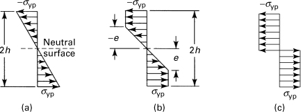
It is clear, upon examining Fig. 12.9b, that the normal stress varies in accordance with the relations
(a)
and
(b)
It is useful to determine the manner in which the bending moment M relates to the distance e. To do this, we begin with a statement of the x equilibrium of forces:
![]()
Cancelling the first and third integrals and combining the remaining integral with Eq. (a), we have
![]()
This expression indicates that the neutral and centroidal axes of the cross section coincide, as in the case of an entirely elastic distribution of stress. Note that in the case of a nonsymmetrical cross section, the neutral axis is generally in a location different from that of the centroidal axis [Ref. 12.5].
Next, the equilibrium of moments about the neutral axis provides the following relation:
![]()
Substituting σx from Eq. (a) into this equation gives the elastic–plastic moment, after integration,
(12.10a)
Alternatively, using Eq. (12.9a), we have
(12.10b)
The general stress distribution is thus defined in terms of the applied moment, inasmuch as e is connected to σx by Eq. (a). For the case in which e = h, Eq. (12.10) reduces to Eq. (12.9) and M = Myp. For e = 0, which applies to a totally plastic beam, Eq. (12.10a) becomes
where Mu is the ultimate moment. It is also referred to as the plastic moment.
Through application of the foregoing analysis, similar relationships can be derived for other cross-sectional shapes. In general, for any cross section, the plastic or ultimate resisting moment for a beam is
(12.12)
where Z is the plastic section modulus. Clearly, for the rectangular beam analyzed here, Z = bh2. The Steel Construction Manual (Sec. 11.7) lists plastic section moduli for many common geometries. Interestingly, the ratio of the ultimate moment to yield moment for a beam depends on the geometric form of the cross section, called the shape factor:
(12.13)
For instance, in the case of a perfectly plastic beam with (b × 2h) with rectangular cross section, we have ![]() and Z = bh2. Substitution of these area properties into the preceding equation results in f = 3/2. Observe that the plastic modulus represents the sum of the first moments of the areas (defined in Sec. C.1) of the cross section above and below the neutral axis z (Fig. 12.7a): Z = bh(h/2 + h/2) = bh2.
and Z = bh2. Substitution of these area properties into the preceding equation results in f = 3/2. Observe that the plastic modulus represents the sum of the first moments of the areas (defined in Sec. C.1) of the cross section above and below the neutral axis z (Fig. 12.7a): Z = bh(h/2 + h/2) = bh2.
As noted earlier, when a beam is bent inelastically, some plastic deformation is produced, and the beam does not return to its initial configuration after load is released. There will be some residual stresses in the beam (see Example 12.7). The foregoing stresses are found by using the principle of superposition in a way similar to that described in Section 12.5 for axial loading. The unloading phase may be analyzed by assuming the beam to be fully plastic, using the flexure formula, Eq. (5.4).
Plastic Hinge
We now consider the moment–curvature relation of an elastoplastic rectangular beam in pure bending (Fig. 12.7a). As described in Section 5.2, the applied bending moment M produces a curvature which is the reciprocal of the radius of curvature r. At the elastic–plastic boundary of the beam (Fig. 12.9b), the yield strain is εx = εyp. Then, Eq. (12.5) leads to
(c)
The quantities 1/r and 1/ryp correspond to the curvatures of the beam after and at the onset of yielding, respectively. Through the use of Eqs. (c),
(12.14)
Carrying Eqs. (12.14) and (12.9) into Eq. (12.10b) give the required moment–curvature relationship in the form:
We note that Eq. (12.15) is valid only if the bending moment becomes greater than Myp. When M < Myp, Eq. (5.9a) applies. The variation of M with curvature is illustrated in Fig. 12.10. Observe that M rapidly approaches the asymptotic value ![]() , which is the plastic moment Mu. If 1/r = 2/ryp or e = h/2, eleven-twelfths of Mu has already been reached. Obviously, positions A, B, and E of the curve correspond to the stress distributions depicted in Fig. 12.9. Removing the load at C, for example, elastic rebound occurs along the line CD, and point D is the residual curvature.
, which is the plastic moment Mu. If 1/r = 2/ryp or e = h/2, eleven-twelfths of Mu has already been reached. Obviously, positions A, B, and E of the curve correspond to the stress distributions depicted in Fig. 12.9. Removing the load at C, for example, elastic rebound occurs along the line CD, and point D is the residual curvature.
Figure 12.10. Moment–curvature relationship for a rectangular beam.
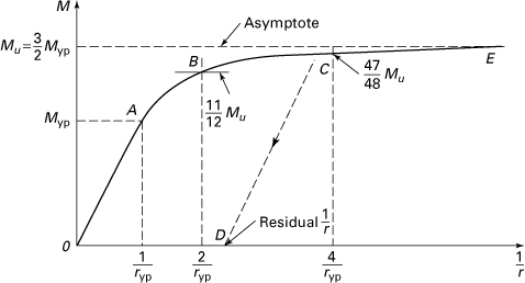
Figure 12.10 depicts the three stages of loading. There is an initial range of linear elastic response. This is followed by a curved line representing the region in which the member is partially plastic and partially elastic. This is the region of contained plastic flow. Finally, the member continues to yield with no increase of applied bending moment. Note the rapid ascent of each curve toward its asymptote as the section approaches the fully plastic condition. At this stage, unrestricted plastic flow occurs and the corresponding moment is the ultimate or plastic hinge moment Mu. Therefore, the cross section will abruptly continue to rotate; the beam is said to have developed a plastic hinge. The rationale for the term hinge becomes apparent upon describing the behavior of a beam under a concentrated loading, discussed next.
Consider a simply supported beam of rectangular cross section, subjected to a load P at its midspan (Fig. 12.11a). The corresponding bending moment diagram is shown in Fig. 12.11b. Clearly, when Myp < |PL/4| < Mu, a region of plastic deformation occurs, as indicated in the figure by the shaded areas. The depth of penetration of these zones can be found from h – e, where e is determined using Eq. (12.10a), because M at midspan is known. The length of the middle portion of the beam where plastic deformation occurs can be readily determined with reference to the figure. The magnitude of bending moment at the edge of the plastic zone is Myp = (P/2) (L – Lp)/2, from which
Figure 12.11. Bending of a rectangular beam: (a) plastic region; (b) moment diagram; (c) plastic hinge.
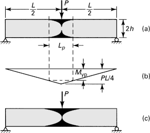
(d)
With the increase of P, Mmax → Mu, and the plastic region extends farther inward. When the magnitude of the maximum moment PL/4 is equal to Mu, the cross section at the midspan becomes fully plastic (Fig. 12.11c). Then, as in the case of pure bending, the curvature at the center of the beam grows without limit, and the beam fails. The beam halves on either side of the midspan experience rotation in the manner of a rigid body about the neutral axis, as about a plastic hinge, under the influence of the constant ultimate moment Mu. For a plastic hinge, P = 4Mu/L is substituted into Eq. (d), leading to Lp = L(1 – Myp/Mu).
The capacity of a beam to resist collapse is revealed by comparing Eqs. (12.9a) and (12.11). Note that the Mu is 1.5 times as large as Myp. Elastic design is thus conservative. Considerations such as this lead to concepts of limit design in structures, discussed in the next section.
Example 12.5. Elastic–Plastic Analysis of a Link: Interaction Curves
A link of rectangular cross section is subjected to a load N (Fig. 12.12a). Derive general relationships involving N and M that govern, first, the case of initial yielding and, then, fully plastic deformation for the straight part of the link of length L.
Figure 12.12. Example 12.5. (a) A link of rectangular cross section carries load P at its ends; (b) elastic stress distribution; (c) fully plastic stress distribution.

Solution
Suppose N and M are such that the state of stress is as shown in Fig. 12.12b at any straight beam section. The maximum stress in the beam is then, by superposition of the axial and bending stresses,
(e)
The upper limits on N (M = 0) and M (N = 0), corresponding to the condition of yielding, are
(f)
Substituting 2hb and I/h from Eq. (f) into Eq. (e) and rearranging terms, we have
(12.16)
If N1 is zero, then M1 must achieve its maximum value Myp for yielding to impend. Similarly, for M1 = 0, it is necessary for N1 to equal Nyp to initiate yielding. Between these extremes, Eq. (12.16) provides the infinity of combinations of N1 and M1 that will result in σyp.
For the fully plastic case (Fig. 12.12c), we shall denote the state of loading by N2 and M2. It is apparent that the stresses acting within the range –e < y < e contribute pure axial load only. The stresses within the range e < y < h and –e > y > –h form a couple, however. For the total load system described, we may write
(g)
(h)
Introducing Eqs. (12.11) and (g) into Eq. (h), we have
![]()
Finally, dividing by Mu and noting that ![]() and Nyp = 2bhσyp, we obtain
and Nyp = 2bhσyp, we obtain
(12.17)
Figure 12.13 is a plot of Eqs. (12.16) and (12.17). By employing these interaction curves, any combination of limiting values of bending moment and axial force is easily arrived at.
Figure 12.13. Example 12.5 (continued). Interaction curves for N and M for a rectangular cross-sectional member.

Let, for instance, d = h, h = 2b = 24 mm (Fig. 12.12a), and σyp = 280 MPa. Then the value of ![]() and, from Eq. (e), Myp/Nyp = h/3 = 8. The radial line representing
and, from Eq. (e), Myp/Nyp = h/3 = 8. The radial line representing ![]() is indicated by the dashed line in the figure. This line intersects the interaction curves at A(0.75, 0.25) and B(1.24, 0.41). Thus, yielding impends for N1 = 0.25Nyp = 0.25 (2bh · σyp) = 40.32 kN, and for fully plastic deformation, N2 = 0.41Nyp = 66.125 kN.
is indicated by the dashed line in the figure. This line intersects the interaction curves at A(0.75, 0.25) and B(1.24, 0.41). Thus, yielding impends for N1 = 0.25Nyp = 0.25 (2bh · σyp) = 40.32 kN, and for fully plastic deformation, N2 = 0.41Nyp = 66.125 kN.
Note that the distance d is assumed constant and the values of N found are conservative. If the link deflection were taken into account, d would be smaller and the calculations would yield larger N.
Example 12.6. Shape Factor of an I-Beam
An I-beam (Fig. 12.14a) is subjected to pure bending resulting from end couples. Determine the moment causing initial yielding and that results in complete plastic deformation.
Figure 12.14. Example 12.6. (a) Cross section; (b) fully plastic stress distribution.
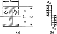
Solution
The moment corresponding to σyp is, from Eq. (12.9a),
![]()
Refer now to the completely plastic stress distribution of Fig. 12.14b. The moments of force owing to σyp, taken about the neutral axis, provide
![]()
Combining the preceding equations, we have
(i)
From this expression, it is seen that ![]() , while it is
, while it is ![]() for a beam of rectangular section (h1 = 0). We conclude, therefore, that if a rectangular beam and an I-beam are designed plastically, the former will be more resistant to complete plastic failure.
for a beam of rectangular section (h1 = 0). We conclude, therefore, that if a rectangular beam and an I-beam are designed plastically, the former will be more resistant to complete plastic failure.
Example 12.7. Residual Stresses in a Rectangular Beam
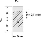
Figure 12.15 shows an elastoplastic beam of rectangular cross section 40 mm by 100 mm carrying a bending moment of M. Determine (a) the thickness of the elastic core; (b) the residual stresses following removal of the bending moment. Given: b = 40 mm, h = 50 mm, M = 21 kN · m, σyp = 240 MPa, and E = 200 GPa.
Figure 12.15. Example 12.7. Finding the thickness (2e) of the elastic core.
Solution
a. Through the use of Eq. (12.9a), we have
![]()
Then Eq. (12.10b) leads to
![]()
e = 31 × 10–3 m = 31 mm and 2e = 62 mm
Elastic core depicted as shaded in Fig. 12.15.
b. The stress distribution corresponding to moment M = 21 kN · m is illustrated in Fig. 12.16a. The release of moment M produces elastic stresses, and the flexure formula applies (Fig. 12.16b). Equation (5.5) is therefore
![]()
Figure 12.16. Example 12.7 (continued). Stress distribution in a rectangular beam: (a) elastic–plastic; (b) elastic rebound; (c) residual.
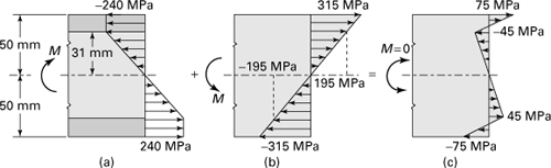
By the superimposition of the two stress distributions, we can find the residual stresses (Fig. 12.16c). Observe that both tensile and compressive residual stresses remain in the beam.
Example 12.8. Deflection of a Perfectly Plastic Simple Beam
Determine the maximum deflection due to an applied force P acting on the perfectly plastic simply supported rectangular beam (Fig. 12.8).
Solution
The center deflection in the elastic range is given by
(j)
At the start of yielding,
(k)
Expression (j), together with Eqs. (k) and (12.9a), leads to
(l)
(m)
for the center deflection at the instant of plastic collapse.
12.8 Collapse Load of Structures: Limit Design
On the basis of the simple examples in the previous section, it may be deduced that structures may withstand loads in excess of those that lead to initial yielding. We recognize that, while such loads need not cause structural collapse, they will result in some amount of permanent deformation. If no permanent deformation is to be permitted, the load configuration must be such that the stress does not attain the yield point anywhere in the structure. This is, of course, the basis of elastic design.
When a limited amount of permanent deformation may be tolerated in a structure, the design can be predicated on higher loads than correspond to initiation of yielding. On the basis of the ultimate or plastic load determination, safe dimensions can be determined in what is termed limit design. Clearly, such design requires higher than usual factors of safety. Examples of ultimate load determination are presented next.
Consider first a built-in beam subjected to a concentrated load at midspan (Fig. 12.17a). The general bending moment variation is sketched in Fig. 12.17b. As the load is progressively increased, we may anticipate plastic hinges at points 1, 2, and 3, because these are the points at which maximum bending moments are found. The configuration indicating the assumed location of the plastic hinges (Fig. 12.17c) is the mechanism of collapse. At every hinge, the hinge moment must clearly be the same.
Figure 12.17. (a) Beam with built-in ends; (b) elastic bending moment diagram; (c) mechanism of collapse with plastic hinges at 1 through 3.

The equilibrium and the energy approaches are available for determination of the ultimate loading. Electing the latter, we refer to Fig. 12.17c and note that the change in energy associated with rotation at points 1 and 2 is Mu · δθ, while at point 3, it is Mu(2δθ). The work done by the concentrated force is P · δv. According to the principle of virtual work, we may write
Pu(δv) = Mu(δθ) + Mu(δθ) + Mu(2δθ) = 4Mu(δθ)
where Pu represents the ultimate load. Because the deformations are limited to small values, it may be stated that ![]() and
and ![]() . Substituting in the preceding expression for δv, it is found that
. Substituting in the preceding expression for δv, it is found that
(a)
where Mu is calculated for a given beam using Eq. (12.12). It is interesting that, by introduction of the plastic hinges, the originally statically indeterminate beam is rendered determinate. The determination of Pu is thus simpler than that of Pyp, on which elastic analysis is based. An advantage of limit design may also be found in noting that a small rotation at either end of the beam or a slight lowering of a support will not influence the value of Pu. Moderate departures from the ideal case, such as these, will, however, have a pronounced effect on the value of Pyp in a statically indeterminate system.
While the positioning of the plastic hinges in the preceding problem is limited to the single possibility shown in Fig. 12.17c, more than one possibility will exist for situations in which several forces act. Correspondingly, a number of collapse mechanisms may exist, and it is incumbent on the designer to select from among them the one associated with the lowest load.
Example 12.9. Collapse Analysis of a Continuous Beam
Determine the collapse load of the continuous beam shown in Fig. 12.18a.
Figure 12.18. Example 12.9. (a) A beam is subjected to loads P and 2P; (b–d) mechanisms of collapse with plastic hinges at 2 through 4.

Solution
The four possibilities of collapse are indicated in Figs. 12.18b through d. We first consider the mechanism of Fig. 12.18b. In this system, motion occurs because of rotations at hinges 1, 2, and 3. The remainder of the beam remains rigid. Applying the principle of virtual work, noting that the moment at point 1 is zero, we have
P(δv) = Mu(2δθ) + Mu(δθ) = 3Mu(δθ)
Because
![]()
this equation yields Pu = 6Mu/L.
For the collapse mode of Fig. 12.18c,
![]()
and thus Pu = 2Mu/L.
The collapse mechanisms indicated by the solid and dashed lines of Fig. 12.18d are unacceptable because they imply a zero bending moment at section 3. We conclude that collapse will occur as in Fig. 12.17c, when P → 2Mu/L.
Example 12.10. Collapse Load of a Continuous Beam
Determine the collapse load of the beam shown in Fig. 12.19a.
Figure 12.19. Example 12.10. (a) Variously loaded beam; (b) mechanism of collapse with plastic hinges at 2 and 3.

Solution
There are a number of collapse possibilities, of which one is indicated in Fig. 12.19b. Let us suppose that there exists a hinge at point 2, a distance e from the left support. Then examination of the geometry leads to θ1 = θ2(L – e)/e or θ1 + θ2 = Lθ2/e. Applying the principle of virtual work,
![]()
or
![]()
from which
(b)
The minimization condition for p in Eq. (b), dp/de = 0, results in
(c)
Thus, Eqs. (b) and (c) provide a possible collapse configuration. The remaining possibilities are similar to those discussed in the previous example and should be checked to ascertain the minimum collapse load.
Determination of the collapse load of frames involves much the same analysis. For complex frames, however, the approaches used in the foregoing examples would lead to extremely cumbersome calculations. For these, special-purpose methods are available to provide approximate solutions [Ref. 12.6].
Example 12.11. Collapse Analysis of a Frame
Apply the method of virtual work to determine the collapse load of the structure shown in Fig. 12.20a. Assume that the rigidity of member BC is 1.2 times greater than that of the vertical members AB and CD.
Figure 12.20. Example 12.11. (a) A frame with concentrated loads; (b and c) mechanism of collapse with plastic hinges at A, B, C, and D.

Solution
Of the several collapse modes, we consider only the two given in Figs. 12.20b and c. On the basis of Fig. 12.20b, plastic hinges will be formed at the ends of the vertical members. Thus, from the principle of virtual work,
![]()
Substituting u = Lθ, this expression leads to Pu = 8Mu/L.
Referring to Fig. 12.20c, we have MuE = 1.2Mu, where Mu is the collapse moment of the vertical elements. Applying the principle of virtual work,
![]()
Noting that u = Lθ and ![]() , this equation provides the following expression for the collapse load: Pu = 2.56Mu/L.
, this equation provides the following expression for the collapse load: Pu = 2.56Mu/L.
12.9 Elastic–Plastic Torsion of Circular Shafts
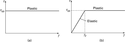
We now consider the torsion of circular bars of ductile materials, which are idealized as elastoplastic, stressed into the plastic range. In this case, the first two basic assumptions associated with small deformations of circular bars in torsion (see Sec. 6.2) are still valid. This means that the circular cross sections remain plane and their radii remain straight. Consequently, strains vary linearly from the shaft axis. The shearing stress–strain curve of plastic materials is shown in Fig. 12.21. Referring to this diagram, we can proceed as discussed before and determine the stress distribution across a section of the shaft for any given value of the torque T.
Figure 12.21. Idealized shear stress–shear strain diagrams for (a) perfectly plastic materials; (b) elastoplastic materials.
The basic relationships given in Section 6.2 are applicable as long as the shear strain in the bar does not exceed the yield strain γyp. It is recalled that the condition of torque equilibrium for the entire shaft (Fig. 6.2) requires
(a)
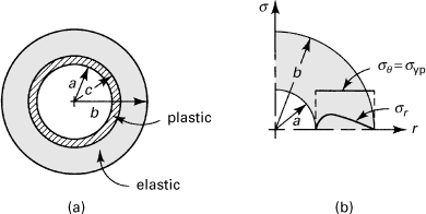
Here ρ, τ are any arbitrary distance and shearing stress from the center O, respectively, and A the entire area of a cross section of the shaft. Increasing in the applied torque, yielding impends on the boundary and moves progressively toward the interior. The cross-sectional stress distribution will be as shown in Fig. 12.22.
Figure 12.22. Stress distribution in a shaft as torque is increased: (a) onset of yield; (b) partially plastic; and (c) fully plastic.

At the start of yielding (Fig. 12.22a), the torque Typ, through the use of Eq. (6.1), may be written in the form:
(12.18)
The quantity J = πc4/2 is the polar moment of inertia for a solid shaft with radius r = c. Equation (12.18) is called the maximum elastic torque, or yield torque. It represents the largest torque for which the deformation remains fully elastic.
If the twist is increased further, an inelastic or plastic portion develops in the bar around an elastic core of radius ρ0 (Fig. 12.22b). Using Eq. (a), we obtain that the torque resisted by the elastic core equals
(b)
The outer portion is subjected to constant yield stress τyp and resists the torque,
(c)
The elastic–plastic or total torque T, the sum of T1 and T2, may now be expressed as follows
(12.19)
When twisting becomes very large, the region of yielding will approach the middle of the shaft and will approach zero (Fig. 12.22c). The corresponding torque Tu is the plastic, or ultimate, shaft torque, and its value from the foregoing equation is
(12.20)
It is thus seen that only one-third of the torque-carrying capacity remains after τyp is reached at the outermost fibers of a shaft.
The radius of elastic core (Fig. 12.22b) is found, referring to Fig. 6.2, by setting γ = γyp and ρ = ρ0. It follows that
(12.21a)
in which L is the length of the shaft. The angle of twist at the onset of yielding φyp (when ρ0 = c) is therefore
(12.21b)
Equations (12.21) lead to the relation,
(12.22)
Using Eq. (12.19), the ultimate torque may then be expressed in the form:
(12.23)
This is valid for φ > φyp. When φ < φyp, linear relation (6.3) applies.
A sketch of Eqs. (6.3) and (12.23) is illustrated in Fig. 12.23. Observe that after yielding torque Typ is reached, T and φ are related nonlinearly. As T approaches Tu, the angle of twist grows without limit. A final point to be noted, however, is that the value of Tu is approached very rapidly (for instance, Tu = 1.32 Typ when φ = 3φyp).
Figure 12.23. Torque–angle of twist relationship for a circular shaft.
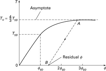
When a shaft is strained beyond the elastic limit (point A in Fig. 12.23) and the applied torque is then removed, rebound is assumed to follow Hooke’s law. Thus, once a portion of a shaft has yielded, residual stresses and residual rotations (φB) will develop. This process and the application of the preceding relationships are demonstrated in Example 12.12. Statically indeterminate, inelastic torsion problems are dealt with similarly to those of axial load, as was discussed in Section 12.5.
Example 12.12. Residual Stress in a Shaft
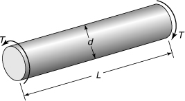
Figure 12.24 shows a solid circular steel shaft of diameter d and length L carrying a torque T. Determine (a) the radius of the elastic core; (b) the angle of twist of the shaft; (c) the residual stresses and the residual rotation when the shaft is unloaded. Assumption: The steel is taken to be an elastoplastic material. Given: d = 60 mm, L = 1.4 m, T = 7.75 kN · m, τyp = 145 MPa, and G = 80 GPa.
Figure 12.24. Example 12.13. Torsion of a circular bar of elastoplastic material.
Solution
We have c = 30 mm and J = π(0.03)4/2 = 1272 × 10–9 m4.
a. Radius of Elastic Core. The yield torque, applying Eq. (12.18), equals
![]()
Equation (12.19), substituting the values of T and τyp, gives
![]()
Solving, ρ0 = 0.604 (30) = 18.1 mm. The elastic–plastic stress distribution in the loaded shaft is illustrated in Fig. 12.25a.
Figure 12.25. Example 5.13 (continued). (a) Partial plastic stresses; (b) elastic rebound stresses; (c) residual stresses.
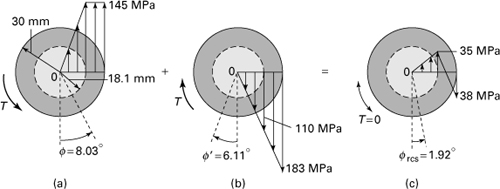
b. Yield Twist Angle. Through the use of Eq. (6.3), the angle of twist at the onset of yielding,
![]()
Introducing the value found for φyp into Eq. (12.22), we have
![]()
c. Residual Stresses and Rotation. The removal of the torque produces elastic stresses as depicted in Fig. 12.25b, and the torsion formula, Eq. (6.1), leads to reversed stress as
![]()
Superposition of the two distributions of stress results in the residual stresses (Fig. 12.25c).
Permanent Twist. The elastic rebound rotation, using Eq. (6.3), equals
![]()
The preceding results indicate that residual rotation of the shaft is
φres = 8.03° – 6.11° = 1.92°
Comment
We see that even though the reversed stresses τ′max exceed the yield strength τyp, the assumption of linear distribution of these stresses is valid, inasmuch as they do not exceed 2τyp.
12.10 Plastic Torsion: Membrane Analogy
Recall from Chapter 6 that the maximum shearing stress in a slender bar of arbitrary section subject to pure torsion is always found on the boundary. As the applied torque is increased, we expect yielding to occur on the boundary and to move progressively toward the interior, as sketched in Fig. 12.26a for a bar of rectangular section. We now determine the ultimate torque Tu that can be carried. This torque corresponds to the totally plastic state of the bar, as was the case of the beams previously discussed. Our analysis treats only perfectly plastic materials.
Figure 12.26. (a) Partially yielded rectangular section; (b) membrane–roof analogy applied to elastic–plastic torsion of a rectangular bar; (c) sand hill analogy applied to plastic torsion of a circular bar.

The stress distribution within the elastic region of the bar is governed by Eq. (6.9),
(12.24)
where Φ represents the stress function (Φ = 0 at the boundary) and θ is the angle of twist. The shearing stresses, in terms of Φ, are
(a)
Inasmuch as the bar is in a state of pure shear, the stress field in the plastic region is, according to the Mises yield criterion, expressed by
(12.25)
where τyp is the yield stress in shear. This expression indicates that the slope of the Φ surface remains constant throughout the plastic region and is equal to τyp.
Membrane–Roof Analogy
Bearing in mind the condition imposed on Φ by Eq. (12.25), the membrane analogy (Sec. 6.6) may be extended from the purely elastic to the elastic–plastic case. As shown in Fig. 12.26b, a roof abc of constant slope is erected with the membrane as its base. Figure 12.26c shows such a roof for a circular section. As the pressure acting beneath the membrane increases, more and more contact is made between the membrane and the roof. In the fully plastic state, the membrane is in total contact with the roof, membrane and roof being of identical slope. Whether the membrane makes partial or complete contact with the roof clearly depends on the pressure. The membrane–roof analogy thus permits solution of elastic–plastic torsion problems.
Sand Hill Analogy
For the case of a totally yielded bar, the membrane–roof analogy leads quite naturally to the sand hill analogy. We need not construct a roof at all, using this method. Instead, sand is heaped on a plate whose outline is cut into the shape of the cross section of the torsion member. The torque is, according to the membrane analogy, proportional to twice the volume of the sand figure so formed. The ultimate torque corresponding to the fully plastic state is thus found.
Referring to Fig. 12.26c, let us apply the sand hill analogy to determine the ultimate torque for a circular bar of radius r. The volume of the corresponding cone is ![]() , where h is the height of the sand hill. The slope h/r represents the yield point stress τyp. The ultimate torque is therefore
, where h is the height of the sand hill. The slope h/r represents the yield point stress τyp. The ultimate torque is therefore
(12.26)
Note that the maximum elastic torque is Typ = (πr3/2)τyp. We may thus form the ratio
(12.27)
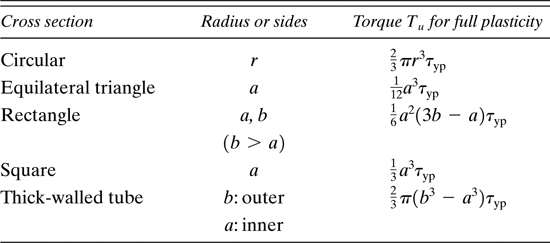
Other solid sections may be treated similarly [Ref. 12.7]. Table 12.1 lists the ultimate torques for bars of various cross-sectional geometry.
Table 12.1. Torque Capacity for Various Common Sections
The procedure may also be applied to members having a symmetrically located hole. In this situation, the plate representing the cross section must contain the same hole as the actual cross section.
12.11 Elastic–Plastic Stresses in Rotating Disks
This section treats the stresses in a flat disk fabricated of a perfectly plastic material, rotating at constant angular velocity. The maximum elastic stresses for this geometry are, from Eqs. (8.30) and (8.28) as follows:
For the solid disk at r = 0,
(a)
For the annular disk at r = a,
(b)
Here a and b represent the inner and outer radii, respectively, ρ the mass density, and ω the angular speed. The following discussion relates to initial, partial, and complete yielding of an annular disk. Analysis of the solid disk is treated in a very similar manner.
Initial Yielding
According to the Tresca yield condition, yielding impends when the maximum stress is equal to the yield stress. Denoting the critical speed as ω0 and using ![]() , we have, from Eq. (b),
, we have, from Eq. (b),
(12.28)
Partial Yielding
For angular speeds in excess of ω0 but lower than speeds resulting in total plasticity, the disk contains both an elastic and a plastic region, as shown in Fig. 12.27a. In the plastic range, the equation of radial equilibrium, Eq. (8.26), with σyp replacing the maximum stress σθ, becomes
Figure 12.27. (a) Partially yielded rotating annular disk; (b) stress distribution in complete yielding.
(12.29)
or
![]()
The solution is given by
(c)
By satisfying the boundary condition σr = 0 at r = a, Eq. (c) provides an expression for the constant c1, which when introduced here results in
(d)
The stress within the plastic region is now determined by letting r = c in Eq. (d):
(12.30)
Referring to the elastic region, the distribution of stress is determined from Eq. (8.27) with σr = σc at r = c, and σr = 0 at r = b. Applying these conditions, we obtain

(e)
The stresses in the outer region are then obtained by substituting Eqs. (e) into Eq. (8.27):

(12.31)
To determine the value of ω that causes yielding up to radius c, we need only substitute σθ for σyp in Eq. (12.31) and introduce σc as given by Eq. (12.30).
Complete Yielding
We turn finally to a determination of the speed ω1 at which the disk becomes fully plastic. First, Eq. (c) is rewritten
(f)
Applying the boundary conditions, σr = 0 at r = a and r = b in Eq. (f), we have
(g)
and the critical speed (ω = ω1) is given by
(12.32)
Substitution of Eqs. (g) and (12.32) into Eq. (f) provides the radial stress in a fully plastic disk:
(12.33)
The distributions of radial and tangential stress are plotted in Fig. 12.27b.
12.12 Plastic Stress–Strain Relations
Consider an element subject to true stresses σ1, σ2, and σ3 with corresponding true straining. The true strain, which is plastic, is denoted ε1, ε2, and ε3. A simple way to derive expressions relating true stress and strain is to replace the elastic constants E and v by Es and ![]() , respectively, in Eqs. (2.34). In so doing, we obtain equations of the total strain theory or the deformational theory, also known as Hencky’s plastic stress–strain relations:
, respectively, in Eqs. (2.34). In so doing, we obtain equations of the total strain theory or the deformational theory, also known as Hencky’s plastic stress–strain relations:

(12.34a)
The foregoing may be restated as
(12.34b)
Here Es, a function of the state of plastic stress, is termed the modulus of plasticity or secant modulus. It is defined by Fig. 12.28
(12.35)
Figure 12.28. True stress–true strain diagram for a rigid-plastic material.
in which the quantities σe and εe are the effective stress and the effective strain, respectively.
Although other yield theories may be employed to determine σe, the maximum energy of distortion or Mises theory (Sec. 4.7) is most suitable. According to the Mises theory, the following relationship connects the uniaxial yield stress to the general state of stress at a point:
(12.36)
where the effective stress σe is also referred to as the von Mises stress. It is assumed that expression (12.36) applies not only to yielding or the beginning of inelastic action (σe = σyp) but to any stage of plastic behavior. That is, σe has the value σyp at yielding, and as inelastic deformation progresses, σe increases in accordance with the right side of Eq. (12.36). Equation (12.36) then represents the logical extension of the yield condition to describe plastic deformation after the yield stress is exceeded.
Collecting terms of Eqs. (12.34), we have
(a)
The foregoing, together with Eqs. (12.35) and (12.36), leads to the definition
(12.37a)
or (on the basis of ε1 + ε2 + ε3 = 0), in different form,
(12.37b)
relating the effective plastic strain and the true strain components. Note that, for simple tension, σ2 = σ3 = 0, ε2 = ε3 = –ε1/2, and Eqs. (12.36) and (12.37) result in
(b)
Therefore, for a given σe, εe can be read directly from true stress–strain diagram (Fig. 12.28).
Hencky’s equations as they appear in Eqs. (12.34) have little utility. To give these expressions generality and convert them to a more convenient form, it is useful to employ the empirical relationship (12.2)
σe = K(εe)n
from which
(c)
The true stress–strain relations, upon substitution of Eqs. (12.36) and (c) into (12.34), then assume the following more useful form:
(12.38a)
(12.38b)
(12.38c)
where α = σ2/σ1 and β = σ3/σ1.
In the case of an elastic material (K = E and n = 1), it is observed that Eqs. (12.38) reduce to the familiar generalized Hooke’s law.
Example 12.13. Analysis of Cylindrical Tube by Hencky’s Relations
A thin-walled cylindrical tube of initial radius ro is subjected to internal pressure p. Assume that the values of ro, p, and the material properties (K and n) are given. Apply Hencky’s relations to determine (a) the maximum allowable stress and (b) the initial thickness to for the cylinder to become unstable at internal pressure p.
Solution
The current radius, thickness, and the length are denoted by r, t, and L, respectively. In the plastic range, the hoop, axial, and radial stresses are
(d)
We thus have α = σ2/σ1 and β = 0 in Eqs. (12.38).
Corresponding to these stresses, the components of true strain are, from Eq. (2.24),

(e)
Based on the constancy of volume, Eq. (12.1), we then have
![]()
or
(f)
The first of Eqs. (e) gives
(g)
The tangential stress, the first of Eqs. (d), is therefore
![]()
from which
(h)
Simultaneous solution of Eqs. (12.38) leads readily to
(i)
Equation (h) then appears as
(j)
For material instability,
![]()
which, upon substitution of ∂ p/∂ σ1 and ∂ p/∂ ε1 derived from Eq. (j), becomes
![]()
or
(k)
In Eqs. (12.38) it is observed that σ1 depends on α and ![]() . That is,
. That is,
(l)
Differentiating, we have
(m)
Expressions (k), (l), and (m) lead to the instability condition:
(12.39)
a. Equating expressions (12.39) and (12.38a), we obtain
![]()
and the true tangential stress is thus
(12.40)
b. On the other hand, Eqs. (d), (f), (g), and (12.38) yield
![]()
From this expression, the required original thickness is found to be
(12.41)
wherein σ1 is given by Eq. (12.40).
In the case under consideration, α = 1/2 and Eqs. (12.39), (12.40), and (12.41) thus become
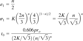
(12.42)
For a thin-walled spherical shell under internal pressure, the two principal stresses are equal and hence α = 1. Equations (12.39), (12.40), and (12.41) then reduce to
(12.43)
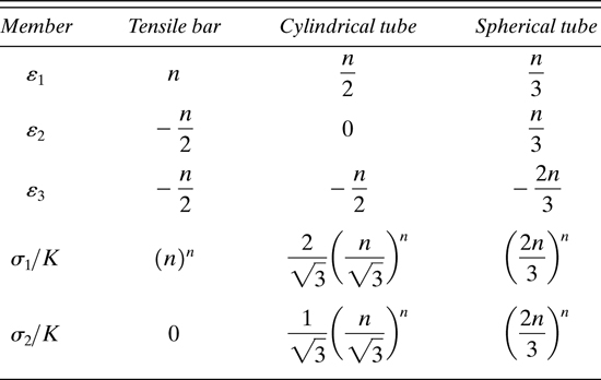
Based on the relations derived in this example, the effective stress and the effective strain are determined readily. Table 12.2 furnishes the maximum true and effective stresses and strains in a thin-walled cylinder and a thin-walled sphere. For purposes of comparison, the table also lists the results (Sec. 12.4) pertaining to simple tension. We observe that at instability, the maximum true strains in a sphere and cylinder are much lower than the corresponding longitudinal strain in uniaxial tension.
Table 12.2. Stress and Strain in Pressurized Plastic Tubes
It is significant that, for loading situations in which the components of stress do not increase continuously, Hencky’s equations provide results that are somewhat in error, and the incremental theory (Sec. 12.13) must be used. Under these circumstances, Eqs. (12.34) or (12.38) cannot describe the complete plastic behavior of the material. The latter is made clearer by considering the following. Suppose that subsequent to a given plastic deformation the material is unloaded, either partially or completely, and then reloaded to a new state of stress that does not result in yielding. We expect no change to occur in the plastic strains; but Hencky’s equations indicate different values of the plastic strain, because the stress components have changed. The latter cannot be valid because during the unloading–loading process, the plastic strains have, in reality, not been affected.
12.13 Plastic Stress–Strain Increment Relations
We have already discussed the limitations of the deformational theory in connection with a situation in which the loading does not continuously increase. The incremental theory offers another approach, treating not the total strain associated with a state of stress but rather the increment of strain.
Suppose now that the true stresses at a point experience very small changes in magnitude dσ1, dσ2, and dσ3. As a consequence of these increments, the effective stress σe will be altered by dσe and the effective strain εe by dεe. The plastic strains thus suffer increments dε1, dε2, and dε3.
The following modification of Hencky’s equations, due to Lévy and Mises, describe the foregoing and give good results in metals:
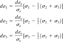
(12.44a)
(12.44b)
The plastic strain is, as before, to occur at constant volume; that is,
dε1 + dε2 + dε3 = 0
The effective strain increment, referring to Eq. (12.37b), may be written
(12.45)
The effective stress σe is given by Eq. (12.36). Alternatively, to ascertain dεe from a uniaxial true stress–strain curve such as Fig. 12.28, it is necessary to know the increase of equivalent stress dσe. Given σe and dεe, it then follows that at any point in the loading process, application of Eqs. (12.44) provides the increment of strain as a unique function of the state of stress and the increment of the stress. According to the Lévy–Mises theory, therefore, the deformation suffered by an element varies in accordance with the specific loading path taken.
In a particular case of straining of sheet metal under biaxial tension, the Lévy–Mises equations (12.44) become
(12.46)
where α = σ2/σ1 and σ3 taken as zero. The effective stress and strain increment, Eqs. (12.36) and (12.45), is now written
(12.47)
(12.48)
Combining Eqs. (12.46) and (12.48) and integrating yields
(12.49)
To generalize this result, it is useful to employ Eq. (12.2), σe = K(εe)n, to include strain-hardening characteristics. Differentiating this expression, we have
(12.50)
Note that, for simple tension, n = εe = ε and Eq. (12.50) reduces to Eq. (12.3).
The utility of the foregoing development is illustrated in Examples 12.14 and 12.15. In closing, we note that the total (elastic–plastic) strains are determined by adding the elastic strains to the plastic strains. The elastic–plastic strain relations, together with the equations of equilibrium and compatibility and appropriate boundary conditions, completely describe a given situation. The general form of the Lévy–Mises relationships, including the elastic incremental components of strain, are referred to as the Prandtl and Reuss equations.
Example 12.14. Analysis of Tube by Lévy–Mises Equations
Redo Example 12.13 employing the Lévy–Mises stress–strain increment relations.
Solution
For the thin-walled cylinder under internal pressure, the plastic stresses are
(a)
where r and t are the current radius and the thickness. At instability,
(b)
Because ![]() , introduction of Eqs. (a) into Eq. (b) provides
, introduction of Eqs. (a) into Eq. (b) provides
(12.51)
Clearly, dr/r is the hoop strain increment dε2, and dt/t is the incremental thickness strain or radial strain increment dε3. Equation (12.51) is the condition of instability for the cylinder material.
Upon application of Eqs. (12.47) and (12.48), the effective stress and the effective strains are found to be

(c)
It is observed that axial strain does not occur and the situation is one of plane strain. The first of Eqs. (c) leads to ![]() , and condition (12.51) gives
, and condition (12.51) gives
![]()
from which
![]()
A comparison of this result with Eq. (12.50) shows that
(12.52)
The true stresses and true strains are then obtained from Eqs. (c) and σe = K(εe)n and the results found to be identical with that obtained using Hencky’s relations (Table 12.2).
For a spherical shell subjected to internal pressure σ1 = σ2 = pr/2t, α = 1 and dε1 = dε2 = –dε3/2. At stability dp = 0, and we now have
(d)
Equations (12.47) and (12.48) result in
(e)
Equations (d) and (e) are combined to yield
(f)
From Eqs. (f) and (12.50), it is concluded that
(12.53)
True stress and true strain are easily obtained, and are the same as the values determined by a different method (Table 12.2).
12.14 Stresses in Perfectly Plastic Thick-Walled Cylinders
The case of a thick-walled cylinder under internal pressure alone was considered in Section 8.2. Equation (8.11) was derived for the onset of yielding at the inner surface of the cylinder owing to maximum shear. This was followed by a discussion of the strengthening of a cylinder by shrinking a jacket on it (Sec. 8.5). The same goal can be achieved by applying sufficient pressure to cause some or all of the material to deform plastically and then releasing the pressure. This is briefly described next [Ref. 12.8].
A continuing increase in internal pressure will result in yielding at the inner surface. As the pressure increases, the plastic zone will spread toward the outer surface, and an elastic–plastic state will prevail in the cylinder with a limiting radius c beyond which the cross section remains elastic. As the pressure increases further, the radius c also increases until, eventually, the entire cross section becomes fully plastic at the ultimate pressure. When the pressure is reduced, the material unloads elastically. Thus, elastic and plastic stresses are superimposed to produce a residual stress pattern (see Example 12.15). The generation of such stresses by plastic action is called autofrettage. Upon reloading, the pressure needed to produce renewed yielding is greater than the pressure that produced initial yielding; the cylinder is thus strengthened by autofrettage.
This section concerns the fully plastic and elastic–plastic actions in a thick-walled cylinder fabricated of a perfectly plastic material of yield strength σyp under internal pressure p as shown in Fig. 12.29a.
Figure 12.29. (a) Thick-walled cylinder of perfectly plastic material under internal pressure; (b) fully plastic stress distribution in the cylinder at the ultimate pressure for b = 4a; (c) partially yielded cylinder.

Complete Yielding
The fully plastic or ultimate pressure as well as the stress distribution corresponding to this pressure is determined by application of the Lévy–Mises relations with σe = σyp. In polar coordinates, the axial strain increment is
(12.54)
If the ends of the cylinder are restrained so that the axial displacement w = 0, the problem may be regarded as a case of plane strain, for which εz = 0. It follows that dεz = 0 and Eq. (12.54) gives
(a)
The equation of equilibrium is, from Eq. (8.2),
(b)
subject to the following boundary conditions:
(c)
Based on the maximum energy of distortion theory of failure, Eqs. (4.4b) or (12.36), setting σ1 = σθ, σ3 = σr, and ![]() results in
results in ![]() . From this, we obtain the yield condition:
. From this, we obtain the yield condition:
(12.55)
Alternatively, according to the maximum shearing stress theory of failure (Sec. 4.6), the yield condition is
(12.56)
Introducing Eq. (12.55) or (12.56) into Eq. (b), we obtain dσr/dr = kσyp/r, which has the solution
(d)
The constant of integration is determined by applying the second of Eqs. (c):
c1 = –kσyp ln b
Equation (d) is thus
(e)
The first of conditions (c) now leads to the ultimate pressure:
(12.57)
An expression for σθ can now be obtained by substituting Eq. (e) into Eqs. (12.55) or (12.56). Consequently, Eq. (a) provides σz. The complete plastic stress distribution for a specified σyp is thus found to be

(12.58)
The stresses given by Eqs. (12.58) are plotted in Fig. 12.29, whereas the distribution of elastic tangential and radial stresses is shown in Fig. 8.4a.
Example 12.15. Residual Stresses in a Pressurized Cylinder
A perfectly plastic closed-ended cylinder (σyp = 400 MPa) with 50- and 100-mm internal and external diameters is subjected to an internal pressure p (Fig. 12.29a). On the basis of the maximum distortion energy theory of failure, determine (a) the complete plastic stresses at the inner surface and (b) the residual tangential and axial stresses at the inner surface when the cylinder is unloaded from the ultimate pressure pu.
Solution
The magnitude of the ultimate pressure is, using Eq. (12.57),
![]()
a. From Eqs. (12.58), with r = a,
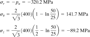
Note, as a check, that σz = (σr + σθ)/2 yields the same result.
b. Unloading is assumed to be linearly elastic. Thus, we have the following elastic stresses at r = a, using Eqs. (8.13) and (8.20):

The residual stresses at the inner surface are therefore
(σθ)res = 141.7 – 533.7 = –392 MPa
(σz)res = –89.2 – 106.7 = –195.9 MPa
The stresses at any other location may be obtained in a like manner.
Partial Yielding
For the elastic segment for which c ≤ r ≤ b (Fig. 12.29c), the tangential and radial stresses are determined using Eqs. (8.12) and (8.13) with a = c. In so doing, we obtain
(12.59a)
(12.59b)
Here pc is the magnitude of the (compressive) radial stress at the elastic–plastic boundary r = c where yielding impends. Accordingly, by substituting these expressions into the yield condition σθ – σr = kσyp, we have
(12.60)
This pressure represents the boundary condition for a fully plastic segment with inner radius a and outer radius c. That is, constant c1 in Eq. (d) is obtained by applying (σr)r = c = –pc:
![]()
Substituting this value of c1 into Eq. (d), the radial stress in the plastic zone becomes
(12.61a)
Then, using the yield condition, the tangential stress in the plastic zone is obtained in the following form:
(12.61b)
Equations (12.59) and (12.61), for a given elastic–plastic boundary radius c, provide the relationships necessary for calculation of the elastic–plastic stress distribution in the cylinder wall (Fig. 12.29c).
References
12.1. FORD, H., Advanced Mechanics of Materials, 2nd ed., Ellis Horwood, Chichester, England, 1977, Part 4.
12.2. FAUPEL, J. H., and FISHER, F. E., Engineering Design, 2nd ed., Wiley, Hoboken, N.J. 1981, Chap. 6.
12.3. MENDELSSON, A., Plasticity: Theory and Applications, Macmillan, New York, 1968 (reprinted, R. E. Krieger, Melbourne, Fla., 1983).
12.4. RAMBERG, W., and OSGOOD, W. R., Description of Stress–Strain Curves by Three Parameters, National Advisory Committee of Aeronautics, TN 902, 1943, Washington, D.C.
12.5. UGURAL, A. C., Mechanics of Materials, Wiley, Hoboken, N.J. 2008, Secs. 4.3 and 7.18.
12.6. HODGE, P C., Plastic Design Analysis of Structures, McGraw-Hill, New York, 1963.
12.7. NADAI, A., Theory of Flow and Fracture of Solids, McGraw-Hill, New York, 1950, Chap. 35.
12.8. HOFFMAN, O., and SACHS, G., Theory of Plasticity for Engineers, McGraw-Hill, New York, 1953.
Problems
Sections 12.1 through 12.6
12.1. A solid circular cylinder of 100-mm diameter is subjected to a bending moment M = 3.375 kN · m, an axial tensile force P = 90 kN, and a twisting end couple T = 4.5 kN · m. Determine the stress deviator tensor. [Hint: Refer to Sec. 2.15.]
12.2. In the pin-connected structure shown in Fig. 12.4, the true stress–engineering strain curves of the members are expressed by ![]() and
and ![]() . Verify that, for all three bars to reach tensile instability simultaneously, they should be set initially at an angle described by
. Verify that, for all three bars to reach tensile instability simultaneously, they should be set initially at an angle described by
(P12.2)
Calculate the value of this initial angle for n1 = 0.2 and n2 = 0.3.
12.3. Determine the deflection of a uniformly loaded rigid-plastic cantilever beam of length L. Locate the origin of coordinates at the fixed end, and denote the loading by p.
12.4. Redo Prob. 12.3 for p = 0 and a concentrated load P applied at the free end.
12.5. Consider a beam of rectangular section, subjected to end moments as shown in Fig. 12.7a. Assuming that the relationship for tensile and compressive stress for the material is approximated by σ = Kε1/4, determine the maximum stress.
12.6. A simply supported rigid-plastic beam is described in Fig. P12.6. Compute the maximum deflection. Reduce the result to the case of a linearly elastic material. ![]() . Let P = 8 kN, E = 200 GPa, L = 1.2 m, and a = 0.45 m. Cross-sectional dimensions shown are in millimeters.
. Let P = 8 kN, E = 200 GPa, L = 1.2 m, and a = 0.45 m. Cross-sectional dimensions shown are in millimeters.

12.7. Figure P12.7 shows a stepped steel bar ABC, axially loaded until it elongates 10 mm, and then unloaded. Determine (a) the largest value of P; (b) the plastic axial deformation of segments AB and BC. Given: d1 = 60 mm, d2 = 50 mm, E = 210 GPa, and σyp = 240 MPa.
12.8. Resolve Prob. 12.7, knowing that d1 = 30 mm, d2 = 20 mm, and σyp = 280 MPa.
12.9. The assembly of three steel bars shown in Fig. 12.4 supports a vertical load P. It can be verified that [see Ref. 12.5], the forces in the bars AD = CD and BD are, respectively,
(P12.9)
Using these equations, calculate the value of ultimate load Pu. Given: Each member is made of mild steel with σyp = 250 MPa and has the same cross-sectional area A = 400 mm2, and α = 40°.
12.10. When a load P = 400 kN is applied and then removed, calculate the residual stress in each bar of the assembly described in Example 12.3.
12.11. Figure P12.11 depicts a cylindrical rod of cross-sectional area A inserted into a tube of the same length L and of cross-sectional area At; the left ends of the members are attached to rigid support and the right ends to a rigid plate. When an axial load P is applied as shown, determine the maximum deflection and draw the load-deflection diagram of the rod–tube assembly. Given: L = 1.2 m, Ar = 45 mm2, At = 60 mm2, Er = 200 GPa, Et = 100 GPa, (σr)yp = 250 MPa, and (σt)yp = 310 MPa. Assumption: The rod and tube are both made of elastoplastic materials.

Sections 12.7 and 12.8
12.12. A ductile bar (σyp = 350 MPa) of square cross section with sides a = 12 mm is subjected to bending moments M about the z axis at its ends (Fig. P12.12). Determine the magnitude of M at which (a) yielding impends; (b) the plastic zones at top and bottom of the bar are 2-mm thick.
12.13. A beam of rectangular cross section (width a, depth h) is subjected to bending moments M at its ends. The beam is constructed of a material displaying the stress–strain relationship shown in Fig. P12.13. What value of M can be carried by the beam?
12.14. A perfectly plastic beam is supported as shown in Fig. P12.14. Determine the maximum deflection at the start of yielding.
12.15. Figure P12.15 shows the cross section of a rectangular beam made of mild steel with σyp = 240 MPa. For bending about the z axis, find (a) the yield moment; (b) the moment producing a e = 20-mm-thick plastic zone at the top and bottom of the beam. Given: b = 60 mm and h = 40 mm.

12.16. A steel rectangular beam, the cross section shown in Fig. P12.15, is subjected to a moment about the z axis 1.3 times greater than M. Calculate (a) the distance from the neutral axis to the point at which elastic core ends, e; (b) the residual stress pattern following release of loading.
12.17. A singly symmetric aluminum beam has the cross section shown in Fig. P12.17. (Dimensions are in millimeters.) Determine the ultimate moment Mu. Assumption: The aluminum is to be elastoplastic with a yield stress of σyp = 260 MPa.
12.18 and 12.19. Find the shape factor f for an elastoplastic beam of the cross sections shown in Figs. P12.18 and P12.19 (Refer to Table C.1).


12.20. A rectangular beam with b = 70 mm and h = 120 mm (Fig. P12.15) is subjected to an ultimate moment Mu. Knowing that σyp = 250 MPa for this beam of ductile material, determine the residual stresses at the upper and lower faces if the loading has been removed.
12.21. Consider a uniform bar of solid circular cross section with radius r, subjected to axial tension and bending moments at both ends. Derive general relationships involving N and M that govern, first, the case of initial yielding and, then, fully plastic deformation. Sketch the interaction curves.
12.22. Figure P12.22 shows a hook made of steel with σyp = 280 MPa, equal in tension and compression. What load P results in complete plastic deformation in section A–B? Neglect the effect of curvature on the stress distribution.

12.23. A propped cantilever beam made of ductile material is loaded as shown in Fig. P12.23. What are the values of the collapse load pu and the distance x?
12.24. Obtain the interaction curves for the beam cross section shown in Fig. 12.14a. The beam is subjected to a bending moment M and an axial load N at both ends. Take b = 2h, b1 = 1.8h, and h1 = 0.7h.
12.25. Obtain the collapse load of the structure shown in Fig. P12.25. Assume that plastic hinges form at 1, 3, and 4.

12.26. What is the collapse load of the beam shown in Fig. P12.26? Assume two possible modes of collapse such that plastic hinges form at 2, 3, and 4.
12.27. A propped cantilever beam AB, made of ductile material, supports a uniform load of intensity p (Fig. P12.27). What is the ultimate limit load pu?
12.28. Figure P12.28 shows two beam cross sections. Determine Mu/Myp for each case.

Sections 12.9 through 12.14
12.29. Figure 12.24 shows a circular elastoplastic shaft with yield strength in shear τyp, shear modulus of elasticity G, diameter d, and length L. The shaft is twisted until the maximum shearing strain equals 6000μ. Determine (a) the magnitude of the corresponding angle of twist φ; (b) the value of the applied torque T. Given: L = 0.5 m, d = 60 mm, G = 70 GPa, and τyp = 180 MPa.
12.30. A circular shaft of diameter d and length L is subjected to a torque of T, as shown in Fig. 12.24. The shaft is made of 6061-T6 aluminum alloy (see Table D.1), which is assumed to be elastoplastic. Find (a) the radius of the elastic core ρ0; (b) the angle of twist φ. Given: d = 25 mm, L = 1.2 m, and T = 4.5 kN · m.
12.31. The fixed-ended shaft illustrated in Fig. P12.31 is made of an elastoplastic material for which the shear modulus of elasticity is G and the yield stress in shear is τyp. Find the magnitude of the applied torque T. Assumption: The angle of twist at step C is φyp = 0.25 rad. Given: a = 2 m, b = 1.5 m, d1 = 80 mm, d2 = 50 mm, G = 80 MPa, and τyp = 240 MPa.

12.32. Determine the elastic–plastic stresses in a rotating solid disk.
12.33. For a rectangular bar of sides a and b, determine the ultimate torque corresponding to the fully plastic state (Table 12.1). Use the sand hill analogy.
12.34. For an equilateral triangular bar of sides 2a, determine (a) the ultimate torque corresponding to the fully plastic state (Table 12.1) (use the sand hill analogy) and (b) the maximum elastic torque by referring to Table 6.2. (c) Compare the results found in (a) and (b).
12.35. An annular disk of equilateral hyperbolic profile with outer and inner radii b and a (Fig. 8.13) is shrunk onto a solid shaft so that the interfacial pressure is pi. Demonstrate that, according to the Tresca yield criterion, when the disk becomes fully plastic,
(P12.35)
Here σyp is the yield point stress and r represents any arbitrary radius.
12.36. Consider a thin-walled cylinder of original radius ro, subjected to internal pressure p. Determine the value of the required original thickness at instability employing Hencky’s relations. Use the following:
![]()
12.37. Redo Example 12.13 for the cylinder under uniform axial tensile load P and p = 0.
12.38. A thin-walled tube of original thickness to and outer radius Ro just fits over a rigid rod of radius ro. Employ the Lévy–Mises relations to verify that the axial load the tube can sustain before instability occurs is represented by
(P12.38)
Assume the tube–rod interface to be frictionless. Use σ = Kεn as the true stress–true strain relationship of the tube material in simple tension.
12.39. A thick-walled cylinder (σyp = 250 MPa) of inner radius a = 50 mm is subjected to an internal pressure of pi = 60 MPa. Determine the outer radius b such as to provide (a) a factor of safety n = 2.5 against yielding; (b) a factor of safety n = 3 against ultimate collapse based on maximum shearing stress theory of failure.
12.40. A thick-walled cylinder has an inner radius a and outer radius b = 2a. What is the internal pressure at which the elastic–plastic boundary is at r = 1.4a, based on maximum energy of distortion criterion? Let σyp = 260 MPa.
12.41. Consider a perfectly plastic pipe (σyp = 420 MPa) having an outer radius of 60 mm and inner radius of 50 mm. Determine the maximum internal pressures at the onset of yielding and for complete yielding on the basis of a factor of safety n = 3 and the following theories of failure: (a) maximum shearing stress and (b) maximum energy of distortion.
12.42. A perfectly plastic, closed-ended cylinder is under internal pressure p (Fig. 12.29a). Applying the maximum shearing stress criterion of failure, calculate the residual stress components at r = 0.25 m when the cylinder is unloaded from pu. Use a = 0.2 m, b = 0.3 m, and σyp = 400 MPa.
12.43. A thick-walled compound cylinder having a = 20 mm, b = 30 mm, and c = 50 mm is subjected to internal pressure. Material yield strengths are 280 MPa and 400 MPa for inner and outer cylinders, respectively. Determine the fully plastic pressure on the basis of the maximum shearing stress criterion of failure.
12.44. A perfectly plastic cylinder for which b/a = 3 is subjected to internal pressure causing yielding of the material to the mid-depth c = (a + b)/2. In terms of k and σyp, determine (a) the pressure between the elastic and plastic zones, (b) the radial stress at r = a, and (c) the tangential stresses at r = b, r = c, and r = a. Note: Relationships derived (Sec. 12.14) depend on the ratios of the radii rather than on their magnitudes. Accordingly, convenient numbers such as a = 1, c = 2, and b = 3 may be employed.