Chapter 4. Failure Criteria
4.1 Introduction
The efficiency of design relies in great measure on an ability to predict the circumstances under which failure is likely to occur. The important variables connected with structural failure include the nature of the material; the load configuration; the rate of loading; the shape, surface peculiarities, and temperature of the member; and the characteristics of the medium surrounding the member (environmental conditions). Exact quantitative formulation of the problem of failure and accurate means for predicting failure represent areas of current research.
In Chapter 2 the stress–strain properties and characteristics of engineering materials were presented. We now discuss the mechanical behavior of materials associated with failure. The relations introduced for each theory are represented in a graphical form, which are extremely useful in visualizing impending failure in a stressed member. Note that a yield criterion is a part of plasticity theory (see Sec. 12.1). An introduction to fracture mechanics theory that provides a means to predict a sudden failure as the basis of a computed stress-intensity factor compared to a tested toughness criterion for the material is given in Section 4.13. Theories of failure for repeated loading and response of materials to dynamic loading and temperature change are taken up in the remaining sections.
4.2 Failure
In the most general terms, failure refers to any action leading to an inability on the part of the structure or machine to function in the manner intended. It follows that permanent deformation, fracture, or even excessive linear elastic deflection may be regarded as modes of failure, the last being the most easily predicted. Another way in which a member may fail is through instability, by undergoing large displacements from its design configuration when the applied load reaches a critical value, the buckling load (Chap. 11). In this chapter, the failure of homogeneous materials by yielding or permanent deformation and by fracture are given particular emphasis.*
Among the variables cited, one of the most important factors in regard to influencing the threshold of failure is the rate at which the load is applied. Loading at high rate, that is, dynamic loading, may lead to a variety of adverse phenomena associated with impact, acceleration, and vibration, and with the concomitant high levels of stress and strain, as well as rapid reversal of stress. In a conventional tension test, the rate referred to may relate to either the application of load or changes in strain. Ordinarily, strain rates on the order of 10–4 s–1 are regarded as “static” loading.
Our primary concern in this chapter and in this text is with polycrystalline structural metals or alloys, which are composed of crystals or grains built up of atoms. It is reasonable to expect that very small volumes of a given metal will not exhibit isotropy in such properties as elastic modulus. Nevertheless, we adhere to the basic assumption of isotrophy and homogeneity, because we deal primarily with an entire body or a large enough segment of the body to contain many randomly distributed crystals, which behave as an isotropic material would.
The brittle or ductile character of a metal has relevance to the mechanism of failure. If a metal is capable of undergoing an appreciable amount of yielding or permanent deformation, it is regarded as ductile. Such materials include mild steel, aluminum and some of its alloys, copper, magnesium, lead, Teflon, and many others. If, prior to fracture, the material can suffer only small yielding (less than 5%), the material is classified as brittle. Examples are concrete, stone, cast iron, glass, ceramic materials, and many common metallic alloys. The distinction between ductile and brittle materials is not as simple as might be inferred from this discussion. The nature of the stress, the temperature, and the material itself all play a role, as discussed in Section 4.17, in defining the boundary between ductility and brittleness.
4.3 Failure by Yielding
Whether because of material inhomogeneity or nonuniformity of loading, regions of high stress may be present in which localized yielding occurs. As the load increases, the inelastic action becomes more widespread, resulting eventually in a state of general yielding. The rapidity with which the transition from localized to general yielding occurs depends on the service conditions as well as the distribution of stress and the properties of the materials. Among the various service conditions, temperature represents a particularly significant factor.
The relative motion or slip between two planes of atoms (and the relative displacement of two sections of a crystal that results) represents the most common mechanism of yielding. Slip occurs most readily along certain crystallographic planes, termed slip or shear planes. The planes along which slip takes place easily are generally those containing the largest number of atoms per unit area. Inasmuch as the gross yielding of material represents the total effect of slip occurring along many randomly oriented planes, the yield strength is clearly a statistical quantity, as are other material properties such as the modulus of elasticity. If a metal fails by yielding, one can, on the basis of the preceding considerations, expect the shearing stress to play an important role.
It is characteristic of most ductile materials that after yielding has taken place, the load must be increased to produce further deformation. In other words, the material exhibits a strengthening termed strain hardening or cold working, as shown in Section 2.8. The slip occurring on intersecting planes of randomly oriented crystals and their resulting interaction is believed to be a factor of prime importance in strain hardening.
Creep
The deformation of a material under short-time loading (as occurs in a simple tension test) is simultaneous with the increase in load. Under certain circumstances, deformation may continue with time while the load remains constant. This deformation, beyond that experienced as the material is initially loaded, is termed creep. Turbine disks and reinforced concrete floors offer examples in which creep may be a problem. In materials such as lead, rubber, and certain plastics, creep may occur at ordinary temperatures. Most metals, on the other hand, begin to evidence a loss of strain hardening and manifest appreciable creep only when the absolute temperature is roughly 35 to 50% of the melting temperature. The rate at which creep proceeds in a given material depends on the stress, temperature, and history of loading.
A deformation time curve (creep curve), as in Fig. 4.1, typically displays a segment of decelerating creep rate (stage 0 to 1), a segment of essentially constant deformation or minimum creep rate (stage 1 to 2), and finally a segment of accelerating creep rate (stage 2 to 3). In the figure, curve A might correspond to a condition of either higher stress or higher temperature than curve B. Both curves terminate in fracture at point 3. The creep strength refers to the maximum employable strength of the material at a prescribed elevated temperature. This value of stress corresponds to a given rate of creep in the second stage (2 to 3), for example, 1% creep in 10,000 hours. Inasmuch as the creep stress and creep strain are not linearly related, calculations involving such material behavior are generally not routine.
Figure 4.1. Typical creep curves for a bar in tension.

Stress relaxation refers to a loss of stress with time at a constant strain or deformation level. It is essentially a relief of stress through the mechanism of internal creep. Bolted flange connections and assemblies with shrink or press fits operating at high temperatures are examples of this variable stress condition. Insight into the behavior of viscoelastic models, briefly described in Section 2.6, can be achieved by subjecting models to standard creep and relaxation tests [Ref. 4.5]. In any event, allowable stresses should be kept low in order to prevent intolerable deformations caused by creep.
4.4 Failure by Fracture
Separation of a material under stress into two or more parts (thereby creating new surface area) is referred to as fracture. The determination of the conditions of combined stress that lead to either elastic or inelastic termination of deformation, that is, predicting the failure strength of a material, is difficult. In 1920, A. A. Griffith was the first to equate the strain energy associated with material failure to that required for the formation of new surfaces. He also concluded that, with respect to its capacity to cause failure, tensile stress represents a more important influence than does compressive stress. The Griffith theory assumes the presence in brittle materials of minute cracks, which as a result of applied stress are caused to grow to macroscopic size, leading eventually to failure.
Although Griffith’s experiments dealt primarily with glass, his results have been widely applied to other materials. Application to metals requires modification of the theory, however, because failure does not occur in an entirely brittle manner. Due to major catastrophic failures of ships, buildings, trains, airplanes, pressure vessels, and bridges in the 1940s and 1950s, increasing attention has been given by design engineers to the conditions of the growth of a crack. Griffith’s concept has been considerably expanded by G. R. Irwin [Ref. 4.6].
Brittle materials most commonly fracture through the grains in what is termed a transcrystalline failure. Here the tensile stress is usually regarded as playing the most significant role. Examination of the failed material reveals very little deformation prior to fracture.
Types of Fracture in Tension
There are two types of fractures to be considered in tensile tests of polycrystalline specimens: brittle fracture, as in the case of cast iron, and shear fracture, as in the case of mild steel, aluminum, and other metals. In the former case, fracture occurs essentially without yielding over a cross section perpendicular to the axis of the specimen. In the latter case, fracture occurs only after considerable plastic stretching and subsequent local reduction of the cross-sectional area (necking) of the specimen, and the familiar cup-and-cone formation is observed.
At the narrowest neck section in cup-and-cone fracture, the tensile forces in the longitudinal fibers exhibit directions, as shown in Fig. 4.2a. The horizontal components of these forces produce radial tangential stresses, so each infinitesimal element is in a condition of three-dimensional stress (Fig. 4.2b). Based on the assumption that plastic flow requires a constant maximum shearing stress, we conclude that the axial tensile stresses σ are nonuniformly distributed over the minimum cross section of the specimen. These stresses have a maximum value σmax at the center of the minimum cross section, where σr and σθ are also maximum, and a minimum value σmin at the surface (Fig. 4.2a). The magnitudes of the maximum and minimum axial stresses depend on the radius a of the minimum cross section and the radius of the curvature r of the neck. The following relationships are used to calculate σmax and σmin [Ref. 4.7]:
(a)
Figure 4.2. Necking of a bar in tension: (a) the distribution of the axial stresses; (b) stress element in the plane of the minimum cross section.

Here σavg = P/πa2 and represents the average stress.
Note that, owing to the condition of three-dimensional stress, the material near the center of the minimum cross section of the tensile specimen has its ductility reduced. During stretching, therefore, the crack begins in that region, while the material near the surface continues to stretch plastically. This explains why the central portion of a cup-and-cone fracture is of brittle character, while near the surface a ductile type of failure is observed.
Progressive Fracture: Fatigue
Multiple application and removal of load, usually measured in thousands of episodes or more, are referred to as repeated loading. Machine and structural members subjected to repeated, fluctuating, or alternating stresses, which are below the ultimate tensile strength or even the yield strength, may nevertheless manifest diminished strength and ductility. Since the phenomenon described, termed fatigue, is difficult to predict and is often influenced by factors eluding recognition, increased uncertainty in strength and in service life must be dealt with [Ref. 4.8]. As is true for brittle behavior in general, fatigue is importantly influenced by minor structural discontinuities, the quality of surface finish, and the chemical nature of the environment.
The types of fracture produced in ductile metals subjected to repeated loading differs greatly from that of fracture under static loading discussed in Section 2.7. In fatigue fractures, two zones of failure can be obtained: the beachmarks (so called because the resemble ripples left on sand by retracting waves) region produced by the gradual development of a crack and the sudden fracture region. As the name suggest, the fracture region is the portion that fails suddenly when the crack reaches its size limit. The appearance of the surfaces of fracture greatly helps in identifying the cause of crack initiation to be corrected in redesign.
A fatigue crack is generally observed to have, as its origin, a point of high stress concentration, for example, the corner of a keyway or a groove. This failure, through the involvement of slip planes and spreading cracks, is progressive in nature. For this reason, progressive fracture is probably a more appropriate term than fatigue failure. Tensile stress, and to a lesser degree shearing stress, lead to fatigue crack propagation, while compressive stress probably does not. The fatigue life or endurance of a material is defined as the number of stress repetitions or cycles prior to fracture. The fatigue life of a given material depends on the magnitudes (and the algebraic signs) of the stresses at the extremes of a stress cycle.
Experimental determination is made of the number of cycles (N) required to break a specimen at a particular stress level (S) under a fluctuating load. From such tests, called fatigue tests, curves termed S–N diagrams can be constructed. Various types of simple fatigue stress-testing machines have been developed. Detailed information on this kind of equipment may be found in publications such as cited in the footnote of Section 4.2. The simplest is a rotating bar fatigue-testing machine on which a specimen (usually of circular cross section) is held so that it rotates while under condition of alternating pure bending. A complete reversal (tension to compression) of stress thus results.
It is usual practice to plot stress versus number of cycles with semilogarithmic scales (that is, σ against log N). For most steels, the S–N diagram obtained in a simple fatigue test performed on a number of nominally identical specimens loaded at different stress levels has the appearance shown in Fig. 4.3. The stress at which the curve levels off is called the fatigue or endurance limit σe. Beyond the point (σe, Ne) failure will not take place no matter how great the number of cycles. For a lower number of cycles N < Nf, the loading is regarded as static. At N = Nf cycles, failure occurs at static tensile fracture stress σf. The fatigue strength for complete stress reversal at a specified number of cycles Ncr, is designated σcr on the diagram. The S–N curve relationships are utilized in Section 4.15, in which combined stress fatigue properties are discussed.
Figure 4.3. Typical S–N diagram for steel.

While yielding and fracture may well depend on the rate of load application or the rate at which the small permanent strains form, we shall, with the exception of Sections 4.16, 4.17, and 12.13, assume that yielding and fracture in solids are functions solely of the states of stress or strain.
4.5 Yield and Fracture Criteria
As the tensile loading of a ductile member is increased, a point is eventually reached at which changes in geometry are no longer entirely reversible. The beginning of inelastic behavior (yield) is thus marked. The extent of the inelastic deformation preceding fracture very much depends on the material involved.
Consider an element subjected to a general state of stress, where σ1 > σ2 > σ3. Recall that subscripts 1, 2, and 3 refer to the principal directions. The state of stress in uniaxial loading is described by σ1, equal to the normal force divided by the cross-sectional area, and σ2 = σ3 = 0. Corresponding to the start of the yielding event in this simple tension test are the quantities pertinent to stress and strain energy shown in the second column of Table 4.1. Note that the items listed in this column, expressed in terms of the uniaxial yield point stress σyp, have special significance in predicting failure involving multiaxial states of stress. In the case of a material in simple torsion, the state of stress is given by τ = σ1 = –σ3 and σ2 = 0. In the foregoing, τ is calculated using the standard torsion formula. Corresponding to this case of pure shear, at the onset of yielding, are the quantities shown in the third column of the table, expressed in terms of yield point stress in torsion, τyp.
Table 4.1. Shear Stress and Strain Energy at the Start of Yielding

The behavior of materials subjected to uniaxial normal stresses or pure shearing stresses is readily presented on stress–strain diagrams. The onset of yielding or fracture in these cases is considerably more apparent than in situations involving combined stress. From the viewpoint of mechanical design, it is imperative that some practical guides be available to predict yielding or fracture under the conditions of stress as they are likely to exist in service. To meet this need and to understand the basis of material failure, a number of failure criteria have been developed. In this chapter we discuss only the classical idealizations of yield and fracture criteria of materials. These strength theories are structured to apply to particular classes of materials. The three most widely accepted theories to predict the onset of inelastic behavior for ductile materials under combined stress are described first in Sections 4.6 through 4.9. This is followed by a presentation of three fracture theories pertaining to brittle materials under combined stress (Secs. 4.10 through 4.12).
In addition to the failure theories, failure is sometimes predicted conveniently using the interaction curves discussed in Section 12.7. Experimentally obtained curves of this kind, unless complicated by a buckling phenomenon, are equivalent to the strength criteria considered here.
4.6 Maximum Shearing Stress Theory
The maximum shearing stress theory is an outgrowth of the experimental observation that a ductile material yields as a result of slip or shear along crystalline planes. Proposed by C. A. Coulomb (1736–1806), it is also referred to as the Tresca yield criterion in recognition of the contribution of H. E. Tresca (1814–1885) to its application. This theory predicts that yielding will start when the maximum shearing stress in the material equals the maximum shearing stress at yielding in a simple tension test. Thus, by applying Eq. (1.45) and Table 4.1, we obtain
![]()
or
(4.1)
In the case of plane stress, σ3 = 0, there are two combinations of stresses to be considered. When σ1 and σ2 are of opposite sign, that is, one tensile and the other compressive, the maximum shearing stress is (σ1 – σ2)/2. Thus, the yield condition is given by
(4.2a)
which may be restated as
(4.2b)
When σ1 and σ2 carry the same sign, the maximum shearing stress equals (σ1 – σ3)/2 = σ1/2. Then, for |σ1| > |σ2| and |σ2| > |σ1|, we have the following yield conditions, respectively:
(4.3)
Figure 4.4 is a plot of Eqs. (4.2) and (4.3). Note that Eq. (4.2) applies to the second and fourth quadrants, while Eq. (4.3) applies to the first and third quadrants. The boundary of the hexagon thus marks the onset of yielding, with points outside the shaded region representing a yielded state. The foregoing describes the Tresca yield condition. Good agreement with experiment has been realized for ductile materials. The theory offers an additional advantage in its ease of application.
Figure 4.4. Yield criterion based on maximum shearing stress.
4.7 Maximum Distortion Energy Theory
The maximum distortion energy theory, also known as the von Mises theory, was proposed by M. T. Huber in 1904 and further developed by R. von Mises (1913) and H. Hencky (1925). In this theory, failure by yielding occurs when, at any point in the body, the distortion energy per unit volume in a state of combined stress becomes equal to that associated with yielding in a simple tension test. Equation (2.65) and Table 4.1 thus lead to
(4.4a)
or, in terms of principal stresses,
(4.4b)
For plane stress σ3 = 0, and the criterion for yielding becomes
(4.5a)
or, alternatively,
(4.5b)
Expression (4.5b) defines the ellipse shown in Fig. 4.5a. We note that, for simplification, Eq. (4.4b) or (4.5a) may be written σe = σyp, where σe is known as the von Mises stress or the effective stress (Sec. 12.12). For example, in the latter case we have ![]() .
.
Figure 4.5. Yield criterion based on distortion energy: (a) plane stress yield ellipse; (b) a state of stress defined by position; (c) yield surface for triaxial state of stress.
Returning to Eq. (4.4b), it is observed that only the differences of the principal stresses are involved. Consequently, addition of an equal amount to each stress does not affect the conclusion with respect to whether or not yielding will occur. In other words, yielding does not depend on hydrostatic tensile or compressive stresses. Now consider Fig. 4.5b, in which a state of stress is defined by the position P(σ1, σ2, σ3) in a principal stress coordinate system as shown. It is clear that a hydrostatic alteration of the stress at point P requires shifting of this point along a direction parallel to direction n, making equal angles with coordinate axes. This is because changes in hydrostatic stress involve changes of the normal stresses by equal amounts. On the basis of the foregoing, it is concluded that the yield criterion is properly described by the cylinder shown in Fig. 4.5c and that the surface of the cylinder is the yield surface. Points within the surface represent states of nonyielding. The ellipse of Fig. 4.5a is defined by the intersection of the cylinder with the σ1, σ2 plane. Note that the yield surface appropriate to the maximum shearing stress criterion (shown by the dashed lines for plane stress) is described by a hexagonal surface placed within the cylinder.
The maximum distortion energy theory of failure finds considerable experimental support in situations involving ductile materials and plane stress. For this reason, it is in common use in design.
4.8 Octahedral Shearing Stress Theory
The octahedral shearing stress theory (also referred to as the Mises–Hencky or simply the von Mises criterion) predicts failure by yielding when the octahedral shearing stress at a point achieves a particular value. This value is determined by the relationship of τoct to σyp in a simple tension test. Referring to Table 4.1, we obtain
(4.6)
where τoct for a general state of stress is given by Eq. (2.66).
The Mises–Hencky criterion may also be viewed in terms of distortion energy [Eq. (2.65)]:
(a)
If it is now asserted that yielding will, in a general state of stress, occur when Uod defined by Eq. (a) is equal to the value given in Table 4.1, then Eq. (4.6) will again be obtained. We conclude, therefore, that the octahedral shearing stress theory enables us to apply the distortion energy theory while dealing with stress rather than energy.
Example 4.1. Circular Shaft under Combined Loads
A circular shaft of tensile strength σyp = 350 MPa is subjected to a combined state of loading defined by bending moment M = 8 kN · m and torque T = 24 kN · m (Fig. 4.6a). Calculate the required shaft diameter d in order to achieve a factor of safety n = 2. Apply (a) the maximum shearing stress theory and (b) the maximum distortion energy theory.
Figure 4.6. Example 4.1. (a) Torsion–flexure of a shaft; (b) Mohr’s circle for torsion–flexure loading.

Solution
For the situation described, the principal stresses are
(b)
where
![]()
Therefore
(4.7)
a. Maximum shearing stress theory: For the state of stress under consideration, it may be observed from Mohr’s circle, shown in Fig. 4.6b, that σ1 is tensile and σ2 is compressive. Thus, through the use of Eqs. (b) and (4.2a),
(4.8a)
or
(4.8b)
After substitution of the numerical values, Eq. (4.8b) gives d = 113.8 mm.
b. Maximum distortion energy theory: From Eqs. (4.5a), (b), and (4.7),
(4.9a)
or
(4.9b)
This result may also be obtained from the octahedral shearing stress theory by applying Eqs. (4.6) and (4.7). Substituting the data into Eq. (4.9b) and solving for d, we have d = 109 mm.
Comments
The diameter based on the shearing stress theory is thus 4.4% larger than that based on the maximum energy of distortion theory. A 114-mm shaft should be used to prevent initiation of yielding.
Example 4.2. Conical Tank filled with Liquid
A steel conical tank, supported at its edges, is filled with a liquid of density γ (Fig. P13.32.). The yield point stress (σyp) of the material is known. The cone angle is 2α. Determine the required wall thickness t of the tank based on a factor of safety n. Apply (a) the maximum shear stress theory and (b) the maximum energy of distortion theory.
Solution
The variations of the circumferential and longitudinal principal, stresses σθ = σ1 and σφ = σ2, in the tank are, respectively (Prob. 13.32),
(c)
These stresses have the largest magnitude:

(d)
a. Maximum shear stress theory: Because σ1 and σ2 are of the same sign and |σ1| > |σ2|, we have, from the first equations of (4.3) and (d),
![]()
The thickness of the tank is found from this equation to be
(e)
b. Maximum distortion energy theory: It is observed in Eq. (d) that the largest values of principal stress are found at different locations. We shall therefore first locate the section at which the combined principal stresses are at a critical value. For this purpose, we insert Eq. (c) into Eq. (4.5a):
(f)
Upon differentiating Eq. (f) with respect to the variable y and equating the result to zero, we obtain
y = 0.52a
Upon substitution of this value of y into Eq. (f), the thickness of the tank is determined:
(g)
Comments
The thickness based on the maximum shear stress theory is thus 10% larger than that based on the maximum energy of distortion theory.
4.9 Comparison of the Yielding Theories
Two approaches may be employed to compare the theories of yielding heretofore discussed. The first comparison equates, for each theory, the critical values corresponding to uniaxial loading and torsion. Referring to Table 4.1, we have

Observe that the difference in strength predicted by these theories is not substantial. A second comparison may be made by means of a superposition of Figs. 4.4 and 4.5a. This is left as an exercise for the reader.
Experiment shows that, for ductile materials, the yield stress obtained from a torsion test is 0.5 to 0.6 times that determined from a simple tension test. We conclude, therefore, that the energy of distortion theory, or the octahedral shearing stress theory, is most suitable for ductile materials. However, the shearing stress theory, which gives τyp = 0.50σyp, is in widespread use because it is simple to apply and offers a conservative result in design.
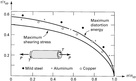
Consider, as an example, a solid shaft of diameter d and tensile yield strength σyp, subjected to combined loading consisting of tension P and torque T. The yield criteria based on the maximum shearing stress and energy of distortion theories, for n = 1, are given by Eqs. (4.8a) and (4.9a):
(a)
where
![]()
A comparison of a dimensionless plot of Eqs. (a) with some experimental results is shown in Fig. 4.7. Note again the particularly good agreement between the maximum distortion energy theory and experimental data for ductile materials.
Figure 4.7. Yield curves for torsion–tension shaft. The points indicated in this figure are based on experimental data obtained by G. I. Taylor and H. Quinney [Ref. 4.9].
4.10 Maximum Principal Stress Theory
According to the maximum principal stress theory, credited to W. J. M. Rankine (1820–1872), a material fails by fracturing when the largest principal stress exceeds the ultimate strength σu in a simple tension test. That is, at the onset of fracture,
(4.10)
Thus, a crack will start at the most highly stressed point in a brittle material when the largest principal stress at that point reaches σu.
Note that, while a material may be weak in simple compression, it may nevertheless sustain very high hydrostatic pressure without fracturing. Furthermore, brittle materials are much stronger in compression than in tension, while the maximum principal stress criterion is based on the assumption that the ultimate strength of a material is the same in tension and compression. Clearly, these are inconsistent with the theory. Moreover, the theory makes no allowance for influences on the failure mechanism other than those of normal stresses. However, for brittle materials in all stress ranges, the maximum principal stress theory has good experimental verification, provided that there exists a tensile principal stress.
In the case of plane stress (σ3 = 0), Eq. (4.10) becomes
(4.11a)
This may be rewritten as
(4.11b)
The foregoing is depicted in Fig. 4.8 with points a, b, and c, d indicating the tensile and compressive principal stresses, respectively. For this case, the boundaries represent the onset of failure due to fracture. The area within the boundary of the figure is thus a region of no failure.
Figure 4.8. Fracture criterion based on maximum principal stress.

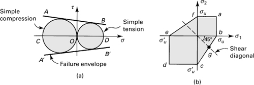
4.11 Mohr’s Theory
The Mohr theory of failure is used to predict the fracture of a material having different properties in tension and compression when results of various types of tests are available for that material. This criterion makes use of the well-known Mohr’s circles of stress. As discussed in Section 1.15, in a Mohr’s circle representation, the shear and normal components of stress acting on a particular plane are specified by the coordinates of a point within the shaded area of Fig. 4.9a. Note that τ depends on σ; that is, |τ| = f(σ).
Figure 4.9. (a) Mohr’s circles of stress; (b) Mohr’s envelopes.

The figure indicates that a vertical line such as PC represents the states of stress on planes with the same σ but with differing τ. It follows that the weakest of all these planes is the one on which the maximum shearing stress acts, designated P. The same conclusion can be drawn regardless of the position of the vertical line between A and B; the points on the outer circle correspond to the weakest planes. On these planes, the maximum and minimum principal stresses alone are sufficient to decide whether or not failure will occur, because these stresses determine the outer circle shown in Fig. 4.9a. Using these extreme values of principal stress thus enables us to apply the Mohr approach to either two- or three-dimensional situations.
The foregoing provides a background for the Mohr theory of failure, which relies on stress plots in σ, τ coordinates. The particulars of the Mohr approach are presented next.
Experiments are performed on a given material to determine the states of stress that result in failure. Each such stress state defines a Mohr’s circle. If the data describing states of limiting stress are derived from only simple tension, simple compression, and pure shear tests, the three resulting circles are adequate to construct the envelope, denoted by lines AB and A′B′ in Fig. 4.9b. The Mohr envelope thus represents the locus of all possible failure states. Many solids, particularly those that are brittle, exhibit greater resistance to compression than to tension. As a consequence, higher limiting shear stresses will, for these materials, be found to the left of the origin, as shown in the figure.
4.12 Coulomb–Mohr Theory
The Coulomb–Mohr or internal friction theory assumes that the critical shearing stress is related to internal friction. If the frictional force is regarded as a function of the normal stress acting on a shear plane, the critical shearing stress and normal stress can be connected by an equation of the following form (Fig. 4.10a):
(a)
Figure 4.10. (a) Straight-line Mohr’s envelopes; (b) Coulomb–Mohr fracture criterion.
The constants a and b represent properties of the particular material. This expression may also be viewed as a straight-line version of the Mohr envelope.
For the case of plane stress, σ3 = 0 when σ1 is tensile and σ2 is compressive. The maximum shearing stress τ and the normal stress σ acting on the shear plane are, from Eqs. (1.22) and (1.23), given by
(b)
Introducing these expressions into Eq. (a), we obtain
(c)
To evaluate the material constants, the following conditions are applied:
(d)
Here σu and ![]() represent the ultimate strength of the material in tension and compression, respectively. If now Eqs. (d) are inserted into Eq. (c), the results are
represent the ultimate strength of the material in tension and compression, respectively. If now Eqs. (d) are inserted into Eq. (c), the results are
![]()
from which
(e)
These constants are now introduced into Eq. (c) to complete the equation of the envelope of failure by fracturing. When this is done, the following expression is obtained, applicable for σ1 > 0, σ2 < 0:
(4.12a)
For any given ratio σ1/σ2, the individual stresses at fracture, σ1 and σ2, can be calculated by applying expression (4.12a) (Prob. 4.22).
Relationships for the case where the principal stresses have the same sign (σ1 > 0, σ2 > 0 or σ1 < 0, σ2 < 0) may be deduced from Fig. 4.10a without resort to the preceding procedure. In the case of biaxial tension (now σmin = σ3 = 0, σ1 and σ2 are tensile), the corresponding Mohr’s circle is represented by diameter OD. Therefore, fracture occurs if either of the two tensile stresses achieves the value σu. That is,
(4.12b)
For biaxial compression (now σmax = σ3 = 0, σ1 and σ2 are compressive), a Mohr’s circle of diameter OC is obtained. Failure by fracture occurs if either of the compressive stresses attains the value ![]() :
:
(4.12c)
Figure 4.10b is a graphical representation of the Coulomb–Mohr theory plotted in the σ1, σ2 plane. Lines ab and af represent Eq. (4.12b), and lines dc and de, Eq. (4.12c). The boundary bc is obtained through the application of Eq. (4.12a). Line ef completes the hexagon in a manner analogous to Fig. 4.4. Points lying within the shaded area should not represent failure, according to the theory. In the case of pure shear, the corresponding limiting point is g. The magnitude of the limiting shear stress may be graphically determined from the figure or calculated from Eq. (4.12a) by letting σ1 = –σ2:
(4.13)
Example 4.3. Tube Torque Requirement
A thin-walled tube is fabricated of a brittle material having ultimate tensile and compressive strengths σu = 300 MPa and ![]() . The radius and thickness of the tube are r = 100 mm and t = 5 mm. Calculate the limiting torque that can be applied without causing failure by fracture. Apply (a) the maximum principal stress theory and (b) the Coulomb–Mohr theory.
. The radius and thickness of the tube are r = 100 mm and t = 5 mm. Calculate the limiting torque that can be applied without causing failure by fracture. Apply (a) the maximum principal stress theory and (b) the Coulomb–Mohr theory.
Solution
The torque and maximum shearing stress are related by the torsion formula:
(f)
The state of stress is described by σ1 = –σ2 = τ, σ3 = 0.
a. Maximum principal stress theory: Equations (4.10) are applied with σ3 replaced by σ2 because the latter is negative: |σ1| = |σ2| = σu. Because we have σ1 = σu = 300 × 106 = τ, from Eq. (f),
T = 314 × 10–6(300 × 106) = 94.2 kN · m
b. Coulomb–Mohr theory: Applying Eq. (4.12a),
![]()
from which τ = 210 MPa. Equation (f) gives T = 314 × 10–6 (210 × 106) = 65.9 kN · m.
Based on the maximum principal stress theory, the torque that can be applied to the tube is thus 30% larger than that based on the Coulomb–Mohr theory. To prevent fracture, the torque should not exceed 65.9 kN · m.
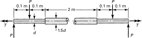
Example 4.4. Design of a Cast Iron Torsion Bar
A torsion-bar spring made of ASTM grade A-48 cast iron is loaded as shown in Fig. 4.11. The stress concentration factors are 1.7 for bending and 1.4 for torsion. Determine the diameter d to resist loads P = 25 N and T = 10 N · m, using a factor of safety n = 2.5. Apply (a) the maximum principal stress theory and (b) the Coulomb–Mohr theory.
Figure 4.11. Example 4.4. A torsion-bar spring.
Solution
The stresses produced by bending moment M = 0.1P and torque T at the shoulder are
(4.14)
The principal stresses, using Eq. (4.7), are then
(4.15)
Substituting the given data, we have
![]()
The foregoing results in
(g)
The allowable ultimate strengths of the material in tension and compression are 170/2.5 = 68 MPa and 650/2.5 = 260 MPa, respectively (see Table D.1).
a. Maximum principal stress theory: On the basis of Eqs. (g) and (4.10),
![]()
Similarly, 52.87/d3 = 68 × 106 gives d = 9.2 mm.
b. Coulomb–Mohr theory: Using Eqs. (g) and (4.12a),
![]()
Comments
The diameter of the spring based on the Coulomb–Mohr theory is therefore about 4.5% larger than that based on the maximum principal stress theory. A 12-mm-diameter bar, a commercial size, should be used to prevent fracture.
4.13 Fracture Mechanics
As noted in Section 4.4, fracture is defined as the separation of a part into two or more pieces. It normally constitutes a “pulling apart” associated with the tensile stress. This type of failure often occurs in some materials in an instant. The mechanisms of brittle fracture are the concern of fracture mechanics, which is based on a stress analysis in the vicinity of a crack or defect of unknown small radius in a part. A crack is a microscopic flaw that may exist under normal conditions on the surface or within the material. These may vary from nonmetallic inclusions and microvoids to weld defects, grinding cracks, and so on. Scratches in the surface due to mishandling can also serve as incipient cracks.
Recall that the stress concentration factors are limited to elastic structures for which all dimensions are precisely known, particularly the radius of the curvature in regions of high stress concentrations. When exists a crack, the stress concentration factor approaches infinity as the root radius approaches 0. Therefore, analysis from the viewpoint of stress concentration factors is inadequate when cracks are present. Space limitations preclude our including more detailed treatment of the subject of fracture mechanics. However, the basic principles and some important results are briefly stated.
The fracture mechanics approach starts with an assumed initial minute crack (or cracks), for which the size, shape, and location can be defined. If brittle failure occurs, it is because the conditions of loading and environment are such that they cause an almost sudden propagation to failure of the original crack. When there is fatigue loading, the initial crack may grow slowly until it reaches a critical size at which the rapid fracture occurs [Ref. 4.8].
Stress-Intensity Factors
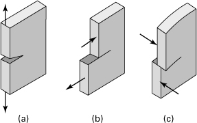
In the fracture mechanics approach, a stress-intensity factor, K, is evaluated. This can be thought of as a measure of the effective local stress at the crack root. The three modes of crack deformation of a plate are shown in Fig. 4.12. The most currently available values of K are for tensile loading normal to the crack, which is called mode I (Fig. 4.12a) and denoted as KI. Modes II and III are essentially associated with the in-plane and out-of-plane loads, respectively (Figs. 4.12b and 4.12c). The treatment here is concerned only with mode I. We eliminate the subscript and let K = KI.
Figure 4.12. Crack deformation types: (a) mode I, opening; (b) mode II, sliding; (c) mode III, tearing.
Solutions for numerous configurations, specific initial crack shapes, and orientations have been developed analytically and by computational techniques, including finite element analysis (FEA) [Ref. 4.10 and 4.11]. For plates and beams, the stress-intensity factor is defined as
(4.16)
In the foregoing, we have σ = normal stress; λ = geometry factor, depends on a/w, listed in Table 4.2; a = crack length (or half crack length); w = member width (or half width of member). It is seen from Eq. (4.16) and Table 4.2 that the stress-intensity factor depends on the applied load and geometry of the specimen as well as on the size and shape of the crack. The units of the stress-intensity factors are commonly MPa ![]() in SI and ksi
in SI and ksi ![]() . in U.S. customary system.
. in U.S. customary system.
Table 4.2. Geometry Factors λ for Initial Crack Shapes

It is obvious that most cracks may not be as basic as shown in Table 4.2. They may be at an angle embedded in a member or sunken into surface. A shallow surface crack in a component may be considered semi-elliptical. A circular or elliptical form has proven to be adequate for many studies. Publications on fracture mechanics provide methods of analysis, applications, and extensive references [Ref. 4.8 through 4.12].
Interestingly, crack propagation occurring after an increase in load may be interrupted if a small zone forms ahead of the crack. However, stress intensity has risen with the increase in crack length and, in time, the crack may advance again a short amount. When stress continues to increase owing to the reduced load-carrying area or different manner, the crack may grow, leading to failure. A final point to be noted is that the stress-intensity factors are also used to predict the rate of growth of a fatigue crack.
4.14 Fracture Toughness
In a toughness test of a given material, the stress-intensity factor at which a crack will propagate is measured. This is the critical stress-intensity factor, referred to as the fracture toughness and denoted by the symbol Kc. Ordinarily, testing is done on an ASTM standard specimen, either a beam or tension member with an edge crack at the root of a notch. Loading is increased slowly, and a record is made of load versus notch opening. The data are interpreted for the value of fracture toughness [Ref. 4.13].
For a known applied stress acting on a member of known or assumed crack length, when the magnitude of stress-intensity factor K reaches fracture toughness Kc, the crack will propagate, leading to rupture in an instant. The factor of safety for fracture mechanics n, strength-to-stress ratio, is thus
(4.17)
Introducing the stress-intensity factor from Eq. (4.16), this becomes
(4.18)
Table 4.3 furnishes the values of the yield strength and fracture toughness for some metal alloys, measured at room temperature in a single edge-notch test specimen.
Table 4.3. Yield Strength σyp and Fatigue Toughness Kc for Some Materials
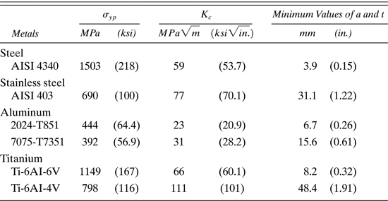
For consistency of results, the ASTM specifications require a crack length a or member thickness t are defined as
(4.19)
This ensures plane strain and flat crack surfaces. The values of a and t found by Eq. (4.19) are also included in Table 4.3.
Application of the foregoing equations is demonstrated in the solution of the following numerical problems.
Example 4.5. Aluminum Bracket with an Edge Crack
A 2024-T851 aluminum alloy frame with an edge crack supports a concentrated load (Fig. 4.13a). Determine the magnitude of the fracture load P based on a safety factor of n = 1.5 for crack length of a = 4 mm. The dimensions are w = 50 mm, d = 125 mm, and t = 25 mm.
Figure 4.13. Example 4.5. Aluminum bracket with an edge crack under a concentrated load.

Solution
From Table 4.3, we have
![]()
Note that that values of a and t both satisfy the table. At the section through the point B (Fig. 4.13b), the bending moment equals M = Pd = 0.125P. Nominal stress, by superposition of two states of stress for axial force P and moment M, is λσ = λaσa + λbσb. Thus
(a)
in which w and t represent the width and thickness of the member, respectively.
The ratio of crack length to bracket width is a/w = 0.08. For cases of B and C of Table 4.2, λa = 1.12 and λb = 1.02, respectively. Substitution of the numerical values into Eq. (4.19) results in

(b)
Therefore, by Eq. (4.17):

The foregoing gives P = 10.61 kN. Note that the normal stress at fracture, 10.61/1(0.05 – 0.004) = 9.226 MPa is well below the yield strength of the material.
Example 4.6. Titanium Panel with a Central Crack
A long plate of width 2w is subjected to a tensile force P in longitudinal direction with a safety factor of n (see case A, Table 4.2). Determine the thickness t required (a) to resist yielding, (b) to prevent a central crack from growing to a length of 2a. Given: w = 50 mm, P = 50 kN, n = 3, and a = 10 mm. Assumption: The plate will be made of Ti-6AI-6V alloy.
Solution
Through the use of Table 4.2, we have ![]() and σyp = 1149 MPa.
and σyp = 1149 MPa.
a. The permissible tensile stress on the basis of the net area is
![]()
Therefore
![]()
b. From the case A of Table 4.2,
![]()
Applying Eq. (4.18), the stress at fracture is

Inasmuch as this stress is smaller than the yield strength, the fracture governs the design; σall = 120.5 MPa. Hence,
![]()
Comment
Use a thickness of 13 mm. Both values of a and t satisfy Table 4.3.
4.15 Failure Criteria for Metal Fatigue
A very common type of fatigue loading consists of an alternating sinusoidal stress superimposed on a uniform stress (Fig. 4.14). Such variation of stress with time occurs, for example, if a forced vibration of constant amplitude is applied to a structural member already transmitting a constant load. Referring to the figure, we define the mean stress and the alternating or range stress as follows:
(4.20)
Figure 4.14. Typical stress–time variation in fatigue.
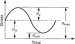
In the case of complete stress reversal, it is clear that the average stress equals zero. The alternating stress component is the most important factor in determining the number of cycles of load the material can withstand before fracture; the mean stress level is less important, particularly if σm is negative (compressive).
As mentioned in Section 4.4, the local character of fatigue phenomena makes it necessary to analyze carefully the stress field within an element. A fatigue crack can start in one small region of high alternating stress and propagate, producing complete failure regardless of how adequately proportioned the remainder of the member may be. To predict whether the state of stress at a critical point will result in failure, a criterion is employed on the basis of the mean and alternating stresses and utilizing the simple S–N curve relationships.
Single Loading
Many approaches have been suggested for interpreting fatigue data. Table 4.4 lists commonly employed criteria, also referred to as mean stress–alternating stress relations. In each case, fatigue strength for complete stress reversal at a specified number of cycles may have a value between the fracture stress and endurance stress; that is, σe ≤ σcr ≤ σf (Fig. 4.3).
Table 4.4.a Failure Criteria for Fatigue

Experience has shown that for steel, the Soderberg or modified Goodman relations are the most reliable for predicting fatigue failure. The Gerber criterion leads to more liberal results and, hence, is less safe to use. For hard steels, the SAE and modified Goodman relations result in identical solutions, since for brittle materials σu = σf.
Relationships presented in Table 4.4 together with specified material properties form the basis for practical fatigue calculations for members under single loading.
Example 4.7. Fatigue Load of Tension-Bending Bar
A square prismatic bar of sides 0.05 m is subjected to an axial thrust (tension) Fm = 90 kN (Fig 4.15). The fatigue strength for completely reversed stress at 106 cycles is 210 MPa, and the static tensile yield strength is 280 MPa. Apply the Soderberg criterion to determine the limiting value of completely reversed axial load Fa that can be superimposed to Fm at the midpoint of a side of the cross section without causing fatigue failure at 106 cycles.
Figure 4.15. Example 4.7. Bar subjected to axial tension Fm and eccentric alternating Fa loads.

Solution
The alternating and mean stresses are given by

Applying the Soderberg criterion,
![]()
we obtain Fa = 152.5 kN.
Combined Loading
Often structural and machine elements are subjected to combined fluctuating bending, torsion, and axial loading. Examples include crankshafts, propeller shafts, and aircraft wings. Under cyclic conditions of a general state of stress, it is common practice to modify the static failure theories for purposes of analysis, substituting the subscripts a, m, and e in the expressions developed in the preceding sections. In so doing, the maximum distortion energy theory, for example, is expressed as
(4.21)
or

(4.22)
Here σea and σem, the equivalent alternating stress and equivalent mean stress, respectively, replace the quantity σyp (or σu) used thus far. Relations for other failure theories can be written in a like manner.
The equivalent mean stress–equivalent alternating stress fatigue failure relations are represented in Table 4.4, replacing σa and σm with σea and σem. These criteria together with modified static failure theories are used to compute fatigue strength under combined loading.
Example 4.8. Fatigue Pressure of a Cylindrical Tank
Consider a thin-walled cylindrical tank of radius r = 120 mm and thickness t = 5 mm, subject to an internal pressure varying from a value of –p/4 to p. Employ the octahedral shear theory together with the Soderberg criterion to compute the value of p producing failure after 108 cycles. The material tensile yield strength is 300 MPa and the fatigue strength is σcr = 250 MPa at 108 cycles.
Solution
The maximum and minimum values of the tangential and axial principal stresses are given by
![]()
![]()
The alternating and mean stresses are therefore

The octahedral shearing stress theory, Eq. (4.6), for cyclic combined stress is expressed as
(4.23)
In terms of computed alternating and mean stresses, Eqs. (4.23) appear as
![]()
from which σea = 12.99p and σem = 7.794p.
The Soderberg relation then leads to
![]()
Solving this equation, p = 12.82 MPa.
Fatigue Life
Combined stress conditions can lower fatigue life appreciably. The approach described here predicts the durability of a structural or machine element loaded in fatigue. The procedure applies to any uniaxial, biaxial, or general state of stress. According to the method, fatigue life Ncr (Fig. 4.3) is defined by the formula*
(4.24)
(4.25)
Here the values of σe and σf are specified in terms of material static tensile strengths, while Ne and Nf are given in cycles (Table 4.5). The fatigue-strength reduction factor K, listed in the table, can be ascertained on the basis of tests or from finite element analysis. The data will be scattered (in general, K > 0.3), and considerable variance requires the stress analyst to use a statistically acceptable value. The reversed stress σcr is computed applying the relations of Table 4.4, as required.
Table 4.5. Fracture Stress σf (Fracture Cycles Nf) and Fatigue Strength σe (Fatigue Life Ne) for Steels

Alternatively, the fatigue life may be determined graphically from the S–N diagram (Fig. 4.3) constructed by connecting points with coordinates (σf, Nf) and (σe, Ne). Interestingly, b represents the slope of the diagram. Following is a solution of a triaxial stress problem illustrating the use of the preceding approach.
Example 4.9. Fatigue Life of an Assembly
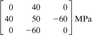
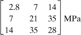
A rotating hub and shaft assembly is subjected to bending moment, axial thrust, bidirectional torque, and a uniform shrink fit pressure so that the following stress levels (in megapascals) occur at an outer critical point of the shaft:

These matrices represent the maximum and minimum stress components, respectively. Determine the fatigue life, using the maximum energy of distortion theory of failure together with (a) the SAE fatigue criterion and (b) the Gerber criterion. The material properties are σu = 2400 MPa and K = 1.
Solution
From Table 4.5, we have σe = 1(2400 × 106)/3 = 800 MPa, Nf = 1 cycle for SAE, Nf = 103 cycles for Gerber, and Ne = 108 cycles. The alternating and mean values of the stress components are

Upon application of Eq. (4.21), the equivalent alternating and mean stresses are found to be
![]()
a. The fatigue strength for complete reversal of stress, referring to Table 4.4, is
![]()
Equation (4.25) yields
![]()
The fatigue life, from Eq. (4.24), is thus
![]()
b. From Table 4.4, we now apply
![]()
and
![]()
![]()
Comment
Upon comparison of the results of (a) and (b), we observe that the Gerber criterion overestimates the fatigue life.
4.16 Impact or Dynamic Loads
Forces suddenly applied to structures and machines are termed shock or impact loads and result in dynamic loading. Examples include rapidly moving loads, such as those caused by a railroad train passing over a bridge or a high-speed rocket-propelled test sled moving on a track, or direct impact loads, such as result from a drop hammer. In machine service, impact loads are due to gradually increasing clearances that develop between mating parts with progressive wear, for example, steering gears and axle journals of automobiles.
A dynamic force acts to modify the static stress and strain fields as well as the resistance properties of a material. Shock loading is usually produced by a sudden application of force or motion to a member, whereas impact loading results from the collision of bodies. When the time of application of a load is equal to or smaller than the largest natural period of vibration of the structural element, shock or impact loading is produced.
Although following a shock or impact loading, vibrations commence, our concern here is only with the influence of impact forces on the maximum stress and deformation of the body. It is important to observe that the design of engineering structures subject to suddenly applied loads is complicated by a number of factors, and theoretical considerations generally serve only qualitatively to guide the design [Ref. 4.18]. Note that the effect of shock loading on members has been neglected in the preceding sections. For example, various failure criteria for metal fatigue result in shaft design equations that include stresses due to fluctuating loads but ignore shock loads. To take into account shock conditions, correction factors should be used in the design equations. The use of static material properties in the design of members under impact loading is regarded as conservative and satisfactory. Details concerning the behavior of materials under impact loading are presented in the next section.
The impact problem is analyzed using the elementary theory together with the following assumptions:
1. The displacement is proportional to the applied forces, static and dynamic.
2. The inertia of a member subjected to impact loading may be neglected.
3. The material behaves elastically. In addition, it is assumed that there is no energy loss associated with the local inelastic deformation occurring at the point of impact or at the supports. Energy is thus conserved within the system.
To idealize an elastic system subjected to an impact force, consider Fig. 4.16, in which is shown a weight W, which falls through a distance h, striking the end of a freestanding spring. As the velocity of the weight is zero initially and is again zero at the instant of maximum deflection of the spring (δmax), the change in kinetic energy of the system is zero, and likewise the work done on the system. The total work consists of the work done by gravity on the mass as it falls and the resisting work done by the spring:
(a)
Figure 4.16. A falling weight W striking a spring.

where k is known as the spring constant.
Note that the weight is assumed to remain in contact with the spring. The deflection corresponding to a static force equal to the weight of the body is simply W/k. This is termed the static deflection, δst. Then the general expression of maximum dynamic deflection is, from Eq. (a),
(4.26)
or, by rearrangement,
(4.27)
The impact factor K, the ratio of the maximum dynamic deflection to the static deflection, δmax/δst, is given by
(4.28)
Multiplication of the impact factor by W yields an equivalent static or dynamic load:
(4.29)
To compute the maximum stress and deflection resulting from impact loading, the preceding load may be used in the relationships derived for static loading.
Two extreme cases are clearly of particular interest. When h ≫ δmax, the work term, Wδmax, in Eq. (a) may be neglected, reducing the expression to ![]() . On the other hand, when h = 0, the load is suddenly applied, and Eq. (a) becomes δmax = 2δst.
. On the other hand, when h = 0, the load is suddenly applied, and Eq. (a) becomes δmax = 2δst.
The expressions derived may readily be applied to analyze the dynamic effects produced by a falling weight causing axial, flexural, or torsional loading. Where bending is concerned, the results obtained are acceptable for the deflections but poor in accuracy for predictions of maximum stress, with the error increasing as h/δst becomes larger or h ≫ δst. This departure is attributable to the variation in the shape of the actual static deflection curve. Thus, the curvature of the beam axis and, in turn, the maximum stress at the location of the impact may differ considerably from that obtained through application of the strength of materials approach.
An analysis similar to the preceding may be employed to derive expressions for the case of a weight W in horizontal motion with a velocity v, arrested by an elastic body. In this instance, the kinetic energy Wv2/2g replaces W(h + δmax), the work done by W, in Eq. (a). Here g is the gravitational acceleration. By so doing, the maximum dynamic load and deflection are found to be, respectively,
(4.30)
where δst is the static deflection caused by a horizontal force W.
Example 4.10. Dynamic Stress and Deflection of a Metal Beam
A weight W = 180 N is dropped a height h = 0.1 m, striking at midspan a simply supported beam of length L = 1.16 m. The beam is of rectangular cross section: a = 25 mm width and b = 75 mm depth. For a material with modulus of elasticity E = 200 GPa, determine the instantaneous maximum deflection and maximum stress for the following cases: (a) the beam is rigidly supported (Fig. 4.17); (b) the beam is supported at each end by springs of stiffness k = 180 kN/m.
Figure 4.17. Example 4.10. A simple beam under center impact due to a falling weight W.

Solution
The deflection of a point at midspan, owing to a statically applied load, is
![]()
The maximum static stress, also occurring at midspan, is calculated from
![]()
a. The impact factor is, from Eq. (4.28),
![]()
We thus have
![]()
b. The static deflection of the beam due to its own bending and the deformation of the spring is
![]()
The impact factor is thus
![]()
Hence,
![]()
Comments
It is observed from a comparison of the results that dynamic loading increases the value of deflection and stress considerably. Also noted is a reduction in stress with increased flexibility attributable to the springs added to the supports. The values calculated for the dynamic stress are probably somewhat high, because h ≫ δst in both cases.
4.17 Dynamic and Thermal Effects
We now explore the conditions under which metals may manifest a change from ductile to brittle behavior, and vice versa. The matter of ductile–brittle transition has important application where the operating environment includes a wide variation in temperature or when the rate of loading changes.
Let us, to begin with, identify two tensile stresses. The first, σf, leads to brittle fracture, that is, failure by cleavage or separation. The second, σy, corresponds to failure by yielding or permanent deformation. These stresses are shown in Fig. 4.18a as functions of material temperature. Referring to the figure, the point of intersection of the two stress curves defines the critical temperature, Tcr. If, at a given temperature above Tcr, the stress is progressively increased, failure will occur by yielding, and the fracture curve will never be encountered. Similarly, for a test conducted at T < Tcr, the yield curve is not intercepted, inasmuch as failure occurs by fracture. The principal factors governing whether failure will occur by fracture or yielding are summarized as follows:
Figure 4.18. Typical transition curves for metals.

Temperature
If the temperature of the specimen exceeds Tcr, resistance to yielding is less than resistance to fracture (σy < σf), and the specimen yields. If the temperature is less than Tcr, then σf < σy, and the specimen fractures without yielding. Note that σf exhibits only a small decrease with increasing temperature.
Loading Rate
Increasing the rate at which the load is applied increases a material’s ability to resist yielding, while leaving comparatively unaffected its resistance to fracture. The increased loading rate thus results in a shift to the position occupied by the dashed curve. Point C moves to C′, meaning that accompanying the increasing loading rate an increase occurs in the critical temperature. In impact tests, brittle fractures are thus observed to occur at higher temperatures than in static tests.
Triaxiality
The effect on the transition of a three-dimensional stress condition, or triaxiality, is similar to that of loading rate. This phenomenon may be illustrated by comparing the tendency to yield in a uniform cylindrical tensile specimen with that of a specimen containing a circumferential groove. The unstressed region above and below the groove tends to resist the deformation associated with the tensile loading of the central region, therefore contributing to a radial stress field in addition to the longitudinal stress. This state of triaxial stress is thus indicative of a tendency to resist yielding (become less ductile), the material behaving in a more brittle fashion.
Referring once more to Fig. 4.18b, in the region to the right of Tcr the material behaves in a ductile manner, while to the left of Tcr it is brittle. At temperatures close to Tcr, the material generally exhibits some yielding prior to a partially brittle fracture. The width of the temperature range over which the transition from brittle to ductile failure occurs is material dependent.
Transition phenomena may also be examined from the viewpoint of the energy required to fracture the material, the toughness rather than the stress (Fig. 4.18b). Notches and grooves serve to reduce the energy required to cause fracture and to shift the transition temperature, normally very low, to the range of normal temperatures. This is one reason that experiments are normally performed on notched specimens.
References
4.1. NADAI, A., Theory of Flow and Fracture of Solids, McGraw-Hill, New York, 1950.
4.2. MARIN, J., Mechanical Behavior of Materials, Prentice Hall, Englewood Cliffs, N.J., 1962.
4.3. VAN VLACK, L. H., Elements of Material Science and Engineering, 6th ed., Addison-Wesley, Reading, Mass., 1989.
4.4. American Society of Metals (ASM), Metals Handbook, Metals Park, Ohio, 1985.
4.5. SHAMES, I. H., and COZZARELLI, F. A., Elastic and Inelastic Stress Analysis, Prentice Hall, Englewood Cliffs, N.J., 1992, Chap. 7.
4.6. IRWIN, G. R., “Fracture Mechanics,” First Symposium on Naval Structural Mechanics, Pergamon, Elmsford, N.Y., 1958, p. 557.
4.7. TIMOSHENKO, S. P., Strength of Materials, Part II, 3rd ed., Van Nostrand, New York, 1956, Chap. 10.
4.8. UGURAL, A. C., Mechanical Design: An Integrated Approach, McGraw-Hill, New York, 2004, Chaps. 7 and 8.
4.9. TAYLOR, G. L., and QUINNEY, H., Philosophical Transactions of the Royal Society, Section A, No. 230, 1931, p. 323.
4.10. KNOTT, J.F., Fundamentals of Fracture Mechanics, Wiley, Hoboken, N.J., 1973.
4.11. BROEK, D., The Practical Use of Fracture Mechanics, Kluwer, Dordrecht, the Netherlands, 1988.
4.12. MEGUID, S.A., Engineering Fracture Mechanics, Elsevier, London, 1989.
4.13. DIETER, G.E., Mechanical Metallurgy, 3rd ed., McGraw-Hill, New York, 1986.
4.14. SULLIVAN, J. L., Fatigue life under combined stress, Mach. Des., January 25, 1979.
4.15. JUVINAL, R. C., and MARSHEK, K. M., Fundamentals of Machine Component Design, 3rd ed., Wiley, Hoboken, N.J., 2000.
4.16. DEUTSCMAN, A. D., MICHELS, W. J., and WILSON, C. E., Machine Design, Theory and Practice, Macmillan, New York, 1975.
4.17. JUVINALL, R.C., Stress, Strain, and Strength, McGraw-Hill, New York, 1967.
4.18. HARRIS, C. M., Shock and Vibration Handbook, McGraw-Hill, New York. 1988.
Problems
Sections 4.1 through 4.9
4.1. A steel circular bar (σyp = 250 MPa) of d = 60-mm diameter is acted upon by combined moments M and axial compressive loads P at its ends. Taking M = 1.5 kN · m, determine, based on the maximum energy of distortion theory of failure, the largest allowable value of P.
4.2. A 5-m-long steel shaft of allowable strength (σall = 100 MPa) supports a torque of T = 325 N · m and its own weight. Find the required shaft diameter d applying the von Mises theory of failure. Assumptions: Use ρ = 7.86 Mg/m3 as the mass per unit volume for steel (see Table D.1). The shaft is supported by frictionless bearings that act as simple supports at its ends.
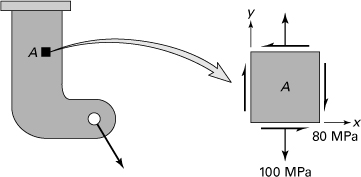
4.3. At a critical point in a loaded ASTM-A36 structural steel bracket, the plane stresses have the magnitudes and directions depicted on element A in Fig. P4.3. Calculate whether the loadings will cause the shaft to fail, based on a safety factor of n = 1.5, applying (a) the maximum shear stress theory; (b) the maximum energy of distortion theory.
4.4. A steel circular cylindrical bar of 0.1-m diameter is subject to compound bending and tension at its ends. The material yield strength is 221 MPa. Assume failure to occur by yielding and take the value of the applied moment to be M = 17 kN · m. Using the octahedral shear stress theory, determine the limiting value of P that can be applied to the bar without causing permanent deformation.
4.5. The state of stress at a critical point in a ASTM-A36 steel member is shown in Fig. P4.5. Determine the factor of safety using (a) the maximum shearing stress criterion; (b) the maximum energy of distortion criterion.

4.6. At a point in a structural member, yielding occurred under a state of stress given by
Determine the uniaxial tensile yield strength of the material according to (a) maximum shearing stress theory, and (b) octahedral shear stress theory.
4.7. A circular shaft of 120-mm diameter is subjected to end loads P = 45 kN, M = 4 kN · m, and T = 11.2 kN · m. Let σyp = 280 MPa. What is the factor of safety, assuming failure to occur in accordance with the octahedral shear stress theory?
4.8. Determine the width t of the cantilever of height 2t and length 0.25 m subjected to a 450-N concentrated force at its free end. Apply the maximum energy of distortion theory. The tensile and compressive strengths of the material are both 280 MPa.
4.9. Determine the required diameter of a steel transmission shaft 10 m in length and of yield strength 350 MPa in order to resist a torque of up to 500 N · m. The shaft is supported by frictionless bearings at its ends. Design the shaft according to the maximum shear stress theory, selecting a factor of safety of 1.5, (a) neglecting the shaft weight, and (b) including the effect of shaft weight. Use γ = 77 kN/m3 as the weight per unit volume of steel.
4.10. The state of stress at a point is described by

Using σyp = 90 MPa, ν = 0.3, and a factor of safety of 1.2, determine whether failure occurs at the point for (a) the maximum shearing stress theory, and (b) the maximum distortion energy theory.
4.11. A solid cylinder of radius 50 mm is subjected to a twisting moment T and an axial load P. Assume that the energy of distortion theory governs and that the yield strength of the material is σyp = 280 MPa. Determine the maximum twisting moment consistent with elastic behavior of the bar for (a) P = 0 and (b) P = 400π kN.
4.12. A simply supported nonmetallic beam of 0.25-m height, 0.1-m width, and 1.5-m span is subjected to a uniform loading of 6 kN/m. Determine the factor of safety for this loading according to (a) the maximum distortion energy theory, and (b) the maximum shearing stress theory. Use σyp = 28 MPa.
4.13. The state of stress at a point in a machine element of irregular shape, subjected to combined loading, is given by

A torsion test performed on a specimen made of the same material shows that yielding occurs at a shearing stress of 9 MPa. Assuming the same ratios are maintained between the stress components, predict the values of the normal stresses σy and σx at which yielding occurs at the point. Use maximum distortion energy theory.
4.14. A steel rod of diameter d = 50 mm (σyp = 260 MPa) supports an axial load P = 50R and vertical load R acting at the end of an 0.8-m-long arm (Fig. P4.14). Given a factor of safety n = 2, compute the largest permissible value of R using the following criteria: (a) maximum shearing stress and (b) maximum energy of distortion.

4.15. Redo Prob. 4.13 for the case in which the stresses at a point in the member are described by

and yielding occurs at a shearing stress of 140 MPa.
4.16. A thin-walled cylindrical pressure vessel of diameter d = 0.5 m and wall thickness t = 5 mm is fabricated of a material with 280-MPa tensile yield strength. Determine the internal pressure p required according to the following theories of failure: (a) maximum distortion energy and (b) maximum shear stress.
4.17. The state of stress at a point is given by
Taking σyp = 82 MPa and a factor of safety of 1.2, determine whether failure takes place at the point, using (a) the maximum shearing stress theory and (b) the maximum distortion energy theory.
4.18. A structural member is subjected to combined loading so that the following stress occur at a critical point:

The tensile yield strength of the material is 300 MPa. Determine the factor of safety n according to (a) maximum shearing stress theory and (b) maximum energy of distortion theory.
4.19. Solve Prob. 4.18 assuming that the state of stress at a critical point in the member is given by

The yield strength is σyp = 220 MPa.
Sections 4.10 through 4.12
4.20. A thin-walled, closed-ended metal tube with ultimate strengths in tension σu and compression ![]() , outer and inner diameters D and d, respectively, is under an internal pressure of p and a torque of T. Calculate the factor of safety n according to the maximum principal stress theory. Given: σu = 250 MPa,
, outer and inner diameters D and d, respectively, is under an internal pressure of p and a torque of T. Calculate the factor of safety n according to the maximum principal stress theory. Given: σu = 250 MPa, ![]() = 520 MPa, D = 210 mm, d = 200 mm, p = 5 MPa, and T = 50 kN · m.
= 520 MPa, D = 210 mm, d = 200 mm, p = 5 MPa, and T = 50 kN · m.
4.21. Design the cross section of a rectangular beam b meters wide by 2b meter deep, supported and uniformly loaded as illustrated in Fig. P4.21. Assumptions: σall = 120 MPa and w = 150 kN/m. Apply the maximum principal stress theory of failure.

4.22. Simple tension and compression tests on a brittle material reveal that failure occurs by fracture at σu = 260 MPa and ![]() , respectively. In an actual application, the material is subjected to perpendicular tensile and compressive stresses, σ1 and σ2, respectively, such that
, respectively. In an actual application, the material is subjected to perpendicular tensile and compressive stresses, σ1 and σ2, respectively, such that ![]() . Determine the limiting values of σ1 and σ2 according to (a) the Mohr theory for an ultimate stress in torsion of τu = 175 MPa and (b) the Coulomb–Mohr theory. [Hint: For case (a), the circle representing the given loading is drawn by a trial-and-error procedure.]
. Determine the limiting values of σ1 and σ2 according to (a) the Mohr theory for an ultimate stress in torsion of τu = 175 MPa and (b) the Coulomb–Mohr theory. [Hint: For case (a), the circle representing the given loading is drawn by a trial-and-error procedure.]
4.23. The state of stress at a point in a cast-iron structure (σu = 290 MPa, ![]() ) is described by σx = 0, σy = –180 MPa, and τxy = 200 MPa. Determine whether failure occurs at the point according to (a) the maximum principal stress criterion and (b) the Coulomb–Mohr criterion.
) is described by σx = 0, σy = –180 MPa, and τxy = 200 MPa. Determine whether failure occurs at the point according to (a) the maximum principal stress criterion and (b) the Coulomb–Mohr criterion.
4.24. A thin-walled cylindrical pressure vessel of 250-mm diameter and 5-mm thickness is subjected to an internal pressure pi = 2.8 MPa, a twisting moment of 31.36 kN · m, and an axial end thrust (tension) P = 45 kN. The ultimate strengths in tension and compression are 210 and 500 MPa, respectively. Apply the following theories to evaluate the ability of the tube to resist failure by fracture: (a) Coulomb–Mohr and (b) maximum principal stress.
4.25. A piece of chalk of ultimate strength σu is subjected to an axial force producing a tensile stress of 3σu/4. Applying the principal stress theory of failure, determine the shear stress produced by a torque that acts simultaneously on the chalk and the orientation of the fracture surface.
4.26. The ultimate strengths in tension and compression of a material are 420 and 900 MPa, respectively. If the stress at a point within a member made of this material is
![]()
determine the factor of safety according to the following theories of failure: (a) maximum principal stress and (b) Coulomb–Mohr.
4.27. A plate, t meters thick, is fabricated of a material having ultimate strengths in tension and compression of σu and ![]() Pa, respectively. Calculate the force P required to punch a hole of d meters in diameter through the plate (Fig. P4.27). Employ (a) the maximum principal stress theory and (b) the Mohr–Coulomb theory. Assume that the shear force is uniformly distributed through the thickness of the plate.
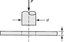
Pa, respectively. Calculate the force P required to punch a hole of d meters in diameter through the plate (Fig. P4.27). Employ (a) the maximum principal stress theory and (b) the Mohr–Coulomb theory. Assume that the shear force is uniformly distributed through the thickness of the plate.
Sections 4.13 through 4.17
4.28. A 2024-T851 aluminum alloy panel, 125-mm wide and 20-mm thick, is loaded in tension in longitudinal direction. Approximate the maximum axial load P that can be applied without causing sudden fracture when an edge crack grows to a 25-mm length (Case B, Table 4.2).
4.29. An AISI 4340 steel ship deck, 10-mm wide and 5-mm thick, is subjected to longitudinal tensile stress of 100 MPa. If a 60-mm-long central transverse crack is present (Case A, Table 4.2), estimate (a) the factor of safety against crack; (b) tensile stress at fracture.
4.30. A long Ti-6Al-6V alloy plate of 130-mm width is loaded by a 200-kN tensile force in longitudinal direction with a safety factor of 2.2. Determine the thickness t required to prevent a central crack to grow to a length of 200 mm (Case A, Table 4.2).
4.31. Resolve Example 4.5 if the frame is made of AISI 4340 steel. Use a = 8 mm, d = 170 mm, w = 40 mm, t = 10 mm, and n = 1.8.
4.32. A 2024-T851 aluminum-alloy plate, w = 150 mm wide and t = 30 mm thick, is under a tensile loading. It has a 24-mm-long transverse crack on one edge (Case B, Table 4.2). Determine the maximum allowable axial load P when the plate will undergo sudden fracture. Also find the nominal stress at fracture.
4.33. An AISI-4340 steel pressure vessel of 60-mm diameter and 5-mm wall thickness contains a 12-mm-long crack (Fig. P4.33). Calculate the pressure that will cause fracture when (a) the crack is longitudinal; (b) the crack is circumferential. Assumption: A factor of safety n = 2 and geometry factor λ = 1.01 are used (Table 4.2).

4.34. A 7075-T7351 aluminum alloy beam with a = 48-mm-long edge crack is in pure bending (see Case D, Table 4.2). Using w = 120 mm and t = 30 mm, find the maximum moment M that can be applied without causing sudden fracture.
4.35. Redo Example 4.7 using the SAE criterion. Take σf = 700 MPa, σcr = 240 MPa, and Fm = 120 kN.
4.36. Redo Example 4.8 employing the maximum shear stress theory together with the Soderberg criterion.
4.37. A bolt is subjected to an alternating axial load of maximum and minimum values Fmax and Fmin. The static tensile ultimate and fatigue strength for completely reversed stress of the material are σu and σcr. Verify that, according to the modified Goodman relation, the expression
(P4.37)
represents the required cross-sectional area of the bolt.
4.38. An electrical contact contains a flat spring in the form of a cantilever beam, b = 5 mm wide by L = 50 mm long by t mm thick, is subjected at its free end to a load P that varies continuously from 0 to 10 N (Fig. P4.38). Employ the Soderberg criterion to calculate the value of t based on yield strength σyp = 1050 MPa, fatigue strength σcr = 510 MPa, and a factor of safety n = 1.5.

4.39. A small leaf spring b = 10 mm wide by L = 125 mm long by t mm thick is simply supported at its ends and subjected to a center load P that varies continuously from 0 to 20 N (Fig. P4.39). Using the modified Goodman criterion, determine the value of t, given a fatigue strength σcr = 740 MPa, ultimate tensile strength σu = 1500 MPa, and safety factor of n = 2.5.

4.40. A circular rotating shaft is subjected to a static bending moment M and a torque that varies from a value of zero to T. Apply the energy of distortion theory together with Soderberg’s relation to obtain the following expression for the required shaft radius:
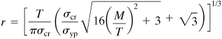
(P4.40)
4.41. Compute the fatigue life of the rotating hub and shaft assembly described in Example 4.9 if at a critical point in the shaft the state of stress is described by σx, max = 1000 MPa, σx, min = –800 MPa, τxy, max = 300 MPa, τxy, min = –100 MPa, and σy = σz = τxz = τyz = 0. Employ the maximum shear stress theory of failure together with the four criteria given in Table 4.4. Take σyp = 1600 MPa, σu = 2400 MPa, and K = 1.
4.42. Determine the fatigue life of a machine element subjected to the following respective maximum and minimum stresses (in megapascals):
![]()
Use the maximum energy of distortion theory of failure together with the (a) modified Goodman criterion and (b) Soderberg criterion. Let σu = 1600 MPa, σyp = 1000 MPa, and K = 1.
4.43. A steel cantilever of width t = 0.05 m, height 2c = 0.1 m, and length L = 1.2 m is subjected to a downward-acting alternating end load of maximum and minimum values Pmax and Pmin = 10 kN. The static tensile yield and fatigue strengths for the completely reversed stress of the material are σyp = 300 MPa and σcr = 200 MPa. Use the Soderberg criterion to determine the value of Pmax that will result in failure.
4.44. A sliding collar of m = 80 kg falls onto a flange at the bottom of a vertical rod (Fig. P4.44). Calculate the height h through which the mass m should drop to produce a maximum stress in the rod of 350 MPa. The rod has length L = 2m, cross-sectional area A = 250 mm2, and modulus of elasticity E = 105 GPa.

4.45. A sliding collar W is dropped from a distance h onto a flange at the bottom of the rod of length L, cross-sectional area A, and modulus of elasticity E (Fig. 4.44). Verify that the weight may be expressed in the form

(P4.45)
in which σmax represents the maximum stress in the rod.
4.46. A 0.125-m-diameter and 1.5-m-long circular shaft has a flywheel at one end and rotates at 240 rpm. The shaft is suddenly stopped at the free end. Determine the maximum shear stress and the maximum angle of twist produced by the impact. It is given that the shaft is made of steel with G = 80.5 GPa, ν = 0.3, the weight of the flywheel is W = 1.09 kN, and the flywheel’s radius of gyration is r = 0.35 m. [Note that kinetic energy Ek = Wω2r2/2g = Tφ/2. Here ω, g, T, φ represent the angular velocity, acceleration of gravity, torque, and angle of twist, respectively.]
4.47. A weight W is dropped from a height h = 0.75 m onto the free end of a cantilever beam of length L = 1.2 m. The beam is of 50-mm by 50-mm square cross section. Determine the value of W required to result in yielding. Omit the weight of the beam. Let σyp = 280 MPa and E = 200 GPa.