Chapter 1. Analysis of Stress
1.1 Introduction
There are two major parts to this chapter. Review of some important fundamentals of statics and mechanics of solids, the concept of stress, modes of load transmission, general sign convention for stress and force resultants that will be used throughout the book, and analysis and design principles are provided first. This is followed with treatment for changing the components of the state of stress given in one set of coordinate axes to any other set of rotated axes, as well as variation of stress within and on the boundaries of a load-carrying member. Plane stress and its transformation are of basic importance, since these conditions are most common in engineering practice. The chapter is thus also a brief guide and introduction to the remainder of the text.
Mechanics of Materials and Theory of Elasticity
The basic structure of matter is characterized by nonuniformity and discontinuity attributable to its various subdivisions: molecules, atoms, and subatomic particles. Our concern in this text is not with the particulate structure, however, and it will be assumed that the matter with which we are concerned is homogeneous and continuously distributed over its volume. There is the clear implication in such an approach that the smallest element cut from the body possesses the same properties as the body. Random fluctuations in the properties of the material are thus of no consequence. This approach is that of continuum mechanics, in which solid elastic materials are treated as though they are continuous media rather than composed of discrete molecules. Of the states of matter, we are here concerned only with the solid, with its ability to maintain its shape without the need of a container and to resist continuous shear, tension, and compression.
In contrast with rigid-body statics and dynamics, which treat the external behavior of bodies (that is, the equilibrium and motion of bodies without regard to small deformations associated with the application of load), the mechanics of solids is concerned with the relationships of external effect (forces and moments) to internal stresses and strains. Two different approaches used in solid mechanics are the mechanics of materials or elementary theory (also called the technical theory) and the theory of elasticity. The mechanics of materials focuses mainly on the more or less approximate solutions of practical problems. The theory of elasticity concerns itself largely with more mathematical analysis to determine the “exact” stress and strain distributions in a loaded body. The difference between these approaches is primarily in the nature of the simplifying assumptions used, described in Section 3.1.
External forces acting on a body may be classified as surface forces and body forces. A surface force is of the concentrated type when it acts at a point; a surface force may also be distributed uniformly or nonuniformly over a finite area. Body forces are associated with the mass rather than the surfaces of a body, and are distributed throughout the volume of a body. Gravitational, magnetic, and inertia forces are all body forces. They are specified in terms of force per unit volume. All forces acting on a body, including the reactive forces caused by supports and body forces, are considered to be external forces. Internal forces are the forces that hold together the particles forming the body. Unless otherwise stated, we assume in this text that body forces can be neglected and that forces are applied steadily and slowly. The latter is referred to as static loading.
In the International System of Units (SI), force is measured in newtons (N). Because the newton is a small quantity, the kilonewton (kN) is often used in practice. In the U.S. Customary System, force is expressed in pounds (lb) or kilopounds (kips). We define all important quantities in both systems of units. However, in numerical examples and problems, SI units are used throughout the text consistent with international convention. (Table D.2 compares the two systems.)
Historical Development
The study of the behavior of members in tension, compression, and bending began with Leonardo da Vinci (1452–1519) and Galileo Galilei (1564–1642). For a proper understanding, however, it was necessary to establish accurate experimental description of a material’s properties. Robert Hooke (1615–1703) was the first to point out that a body is deformed subject to the action of a force. Sir Isaac Newton (1642–1727) developed the concepts of Newtonian mechanics that became key elements of the strength of materials.
Leonard Euler (1707–1783) presented the mathematical theory of columns in 1744. The renowned mathematician Joseph-Louis Lagrange (1736–1813) received credit in developing a partial differential equation to describe plate vibrations. Thomas Young (1773–1829) established a coefficient of elasticity, Young’s modulus. The advent of railroads in the late 1800s provided the impetus for much of the basic work in this area. Many famous scientists and engineers, including Coulomb, Poisson, Navier, St. Venant, Kirchhoff, and Cauchy, were responsible for advances in mechanics of materials during the eighteenth and nineteenth centuries. The British physicist William Thomas Kelvin (1824–1907), better known by his knighted name, Sir Lord Kelvin, first demonstrated that torsional moments acting at the edges of plates could be decomposed into shearing forces. The prominent English mathematician Augustus Edward Hough Love (1863–1940) introduced simple analysis of shells, known as Love’s approximate theory.
Over the years, most basic problems of solid mechanics had been solved. Stephan P. Timoshenko (1878–1972) made numerous original contributions to the field of applied mechanics and wrote pioneering textbooks on the mechanics of materials, theory of elasticity, and theory of elastic stability. The theoretical base for modern strength of materials had been developed by the end of the nineteenth century. Following this, problems associated with the design of aircraft, space vehicles, and nuclear reactors have led to many studies of the more advanced phases of the subject. Consequently, the mechanics of materials is being expanded into the theories of elasticity and plasticity.
In 1956, Turner, Clough, Martin, and Topp introduced the finite element method, which permits the numerical solution of complex problems in solid mechanics in an economical way. Many contributions in this area are owing to Argyris and Zienkiewicz. The recent trend in the development is characterized by heavy reliance on high-speed computers and by the introduction of more rigorous theories. Numerical methods presented in Chapter 7 and applied in the chapters following have clear application to computation by means of electronic digital computers. Research in the foregoing areas is ongoing, not only to meet demands for treating complex problems but to justify further use and limitations on which the theory of solid mechanics is based. Although a widespread body of knowledge exists at present, mechanics of materials and elasticity remain fascinating subjects as their areas of application are continuously expanded.* The literature dealing with various aspects of solid mechanics is voluminous. For those seeking more thorough treatment, selected references are identified in brackets and compiled at the end of each chapter.
1.2 Scope of Treatment
As stated in the preface, this book is intended for advanced undergraduate and graduate engineering students as well as engineering professionals. To make the text as clear as possible, attention is given to the fundamentals of solid mechanics and chapter objectives. A special effort has been made to illustrate important principles and applications with numerical examples. Emphasis is placed on a thorough presentation of several classical topics in advanced mechanics of materials and applied elasticity and of selected advanced topics. Understanding is based on the explanation of the physical behavior of members and then modeling this behavior to develop the theory.
The usual objective of mechanics of material and theory of elasticity is the examination of the load-carrying capacity of a body from three standpoints: strength, stiffness, and stability. Recall that these quantities relate, respectively, to the ability of a member to resist permanent deformation or fracture, to resist deflection, and to retain its equilibrium configuration. For instance, when loading produces an abrupt shape change of a member, instability occurs; similarly, an inelastic deformation or an excessive magnitude of deflection in a member will cause malfunction in normal service. The foregoing matters, by using the fundamental principles (Sec. 1.3), are discussed in later chapters for various types of structural members. Failure by yielding and fracture of the materials under combined loading is taken up in detail in Chapter 4.
Our main concern is the analysis of stress and deformation within a loaded body, which is accomplished by application of one of the methods described in the next section. For this purpose, the analysis of loads is essential. A structure or machine cannot be satisfactory unless its design is based on realistic operating loads. The principal topics under the heading of mechanics of solids may be summarized as follows:
1. Analysis of the stresses and deformations within a body subject to a prescribed system of forces. This is accomplished by solving the governing equations that describe the stress and strain fields (theoretical stress analysis). It is often advantageous, where the shape of the structure or conditions of loading preclude a theoretical solution or where verification is required, to apply the laboratory techniques of experimental stress analysis.
2. Determination by theoretical analysis or by experiment of the limiting values of load that a structural element can sustain without suffering damage, failure, or compromise of function.
3. Determination of the body shape and selection of the materials that are most efficient for resisting a prescribed system of forces under specified conditions of operation such as temperature, humidity, vibration, and ambient pressure. This is the design function.
The design function, item 3, clearly relies on the performance of the theoretical analyses under items 1 and 2, and it is to these that this text is directed. Particularly, emphasis is placed on the development of the equations and methods by which detailed analysis can be accomplished.
The ever-increasing industrial demand for more sophisticated structures and machines calls for a good grasp of the concepts of stress and strain and the behavior of materials—and a considerable degree of ingenuity. This text, at the very least, provides the student with the ideas and information necessary for an understanding of the advanced mechanics of solids and encourages the creative process on the basis of that understanding. Complete, carefully drawn free-body diagrams facilitate visualization, and these we have provided, all the while knowing that the subject matter can be learned best only by solving problems of practical importance. A thorough grasp of fundamentals will prove of great value in attacking new and unfamiliar problems.
1.3 Analysis and Design
Throughout this text, a fundamental procedure for analysis in solving mechanics of solids problems is used repeatedly. The complete analysis of load-carrying structural members by the method of equilibrium requires consideration of three conditions relating to certain laws of forces, laws of material deformation, and geometric compatibility. These essential relationships, called the basic principles of analysis, are:
1. Equilibrium Conditions. The equations of equilibrium of forces must be satisfied throughout the member.
2. Material Behavior. The stress–strain or force-deformation relations (for example, Hooke’s law) must apply to the material behavior of which the member is constructed.
3. Geometry of Deformation. The compatibility conditions of deformations must be satisfied: that is, each deformed portion of the member must fit together with adjacent portions. (Matter of compatibility is not always broached in mechanics of materials analysis.)
The stress and deformation obtained through the use of the three principles must conform to the conditions of loading imposed at the boundaries of a member. This is known as satisfying the boundary conditions. Applications of the preceding procedure are illustrated in the problems presented as the subject unfolds. Note, however, that it is not always necessary to execute an analysis in the exact order of steps listed previously.
As an alternative to the equilibrium methods, the analysis of stress and deformation can be accomplished by employing energy methods (Chap. 10), which are based on the concept of strain energy. The aspect of both the equilibrium and the energy approaches is twofold. These methods can provide solutions of acceptable accuracy where configurations of loading and member shape are regular, and they can be used as the basis of numerical methods (Chap. 7) in the solution of more realistic problems.
Engineering design is the process of applying science and engineering techniques to define a structure or system in detail to allow its realization. The objective of a mechanical design procedure includes finding of proper materials, dimensions, and shapes of the members of a structure or machine so that they will support prescribed loads and perform without failure. Machine design is creating new or improved machines to accomplish specific purposes. Usually, structural design deals with any engineering discipline that requires a structural member or system.
Design is the essence, art, and intent of engineering. A good design satisfies performance, cost, and safety requirements. An optimum design is the best solution to a design problem within given restrictions. Efficiency of the optimization may be gaged by such criteria as minimum weight or volume, optimum cost, and/or any other standard deemed appropriate. For a design problem with many choices, a designer may often make decisions on the basis of experience, to reduce the problem to a single variable. A solution to determine the optimum result becomes straightforward in such a situation.
A plan for satisfying a need usually includes preparation of individual preliminary design. Each preliminary design involves a thorough consideration of the loads and actions that the structure or machine has to support. For each situation, an analysis is necessary. Design decisions, or choosing reasonable values of the safety factors and material properties, are significant in the preliminary design process.
The role of analysis in design may be observed best in examining the phases of a design process. This text provides an elementary treatment of the concept of “design to meet strength requirements” as those requirements relate to individual machine or structural components. That is, the geometrical configuration and material of a component are preselected and the applied loads are specified. Then, the basic formulas for stress are employed to select members of adequate size in each case. The following is rational procedure in the design of a load-carrying member:
1. Evaluate the most likely modes of failure of the member. Failure criteria that predict the various modes of failure under anticipated conditions of service are discussed in Chapter 4.
2. Determine the expressions relating applied loading to such effects as stress, strain, and deformation. Often, the member under consideration and conditions of loading are so significant or so amenable to solution as to have been the subject of prior analysis. For these situations, textbooks, handbooks, journal articles, and technical papers are good sources of information. Where the situation is unique, a mathematical derivation specific to the case at hand is required.
3. Determine the maximum usable value of stress, strain, or energy. This value is obtained either by reference to compilations of material properties or by experimental means such as simple tension test and is used in connection with the relationship derived in step 2.
4. Select a design factor of safety. This is to account for uncertainties in a number of aspects of the design, including those related to the actual service loads, material properties, or environmental factors. An important area of uncertainty is connected with the assumptions made in the analysis of stress and deformation. Also, we are not likely to have a secure knowledge of the stresses that may be introduced during machining, assembly, and shipment of the element.
The design factor of safety also reflects the consequences of failure; for example, the possibility that failure will result in loss of human life or injury or in costly repairs or danger to other components of the overall system. For these reasons, the design factor of safety is also sometimes called the factor of ignorance. The uncertainties encountered during the design phase may be of such magnitude as to lead to a design carrying extreme weight, volume, or cost penalties. It may then be advantageous to perform thorough tests or more exacting analysis rather to rely on overly large design factors of safety.
The true factor of safety, usually referred to simply as the factor of safety, can be determined only after the member is constructed and tested. This factor is the ratio of the maximum load the member can sustain under severe testing without failure to the maximum load actually carried under normal service conditions, the working load. When a linear relationship exists between the load and the stress produced by the load, the factor of safety n may be expressed as
(1.1)
Maximum usable stress represents either the yield stress or the ultimate stress. The allowable stress is the working stress. The factor of safety must be greater than 1.0 if failure is to be avoided. Values for factor of safety, selected by the designer on the basis of experience and judgment, are about 1.5 or greater. For most applications, appropriate factors of safety are found in various construction and manufacturing codes.
The foregoing procedure is not always conducted in as formal a fashion as may be implied. In some design procedures, one or more steps may be regarded as unnecessary or obvious on the basis of previous experience. Suffice it to say that complete design solutions are not unique, involve a consideration of many factors, and often require a trial-and-error process [Ref. 1.6]. Stress is only one consideration in design. Other phases of the design of components are the prediction of the deformation of a given component under given loading and the consideration of buckling (Chap. 11). The methods of determining deformation are discussed in later chapters. Note that there is a very close relationship between analysis and design, and the examples and problems that appear throughout this book illustrate that connection.
We conclude this section with an appeal for the reader to exercise a degree of skepticism with regard to the application of formulas for which there is uncertainty as to the limitations of use or the areas of applicability. The relatively simple form of many formulas usually results from rather severe restrictions in its derivation. These relate to simplified boundary conditions and shapes, limitations on stress and strain, and the neglect of certain complicating factors. Designers and stress analysts must be aware of such restrictions lest their work be of no value or, worse, lead to dangerous inadequacies.
In this chapter, we are concerned with the state of stress at a point and the variation of stress throughout an elastic body. The latter is dealt with in Sections 1.8 and 1.16 and the former in the balance of the chapter.
1.4 Conditions of Equilibrium
A structure is a unit consisting of interconnected members supported in such a way that it is capable of carrying loads in static equilibrium. Structures are of four general types: frames, trusses, machines, and thin-walled (plate and shell) structures. Frames and machines are structures containing multiforce members. The former support loads and are usually stationary, fully restrained structures. The latter transmit and modify forces (or power) and always contain moving parts. The truss provides both a practical and economical solution, particularly in the design of bridges and buildings. When the truss is loaded at its joints, the only force in each member is an axial force, either tensile or compressive.
The analysis and design of structural and machine components require a knowledge of the distribution of forces within such members. Fundamental concepts and conditions of static equilibrium provide the necessary background for the determination of internal as well as external forces. In Section 1.6, we shall see that components of internal-forces resultants have special meaning in terms of the type of deformations they cause, as applied, for example, to slender members. We note that surface forces that develop at support points of a structure are called reactions. They equilibrate the effects of the applied loads on the structures.
The equilibrium of forces is the state in which the forces applied on a body are in balance. Newton’s first law states that if the resultant force acting on a particle (the simplest body) is zero, the particle will remain at rest or will move with constant velocity. Statics is concerned essentially with the case where the particle or body remains at rest. A complete free-body diagram is essential in the solution of problems concerning the equilibrium.
Let us consider the equilibrium of a body in space. In this three-dimensional case, the conditions of equilibrium require the satisfaction of the following equations of statics:
(1.2)
The foregoing state that the sum of all forces acting on a body in any direction must be zero; the sum of all moments about any axis must be zero.
In a planar problem, where all forces act in a single (xy) plane, there are only three independent equations of statics:
(1.3)
That is, the sum of all forces in any (x, y) directions must be zero, and the resultant moment about axis z or any point A in the plane must be zero. By replacing a force summation with an equivalent moment summation in Eqs. (1.3), the following alternative sets of conditions are obtained:
(1.4a)
provided that the line connecting the points A and B is not perpendicular to the x axis, or
(1.4b)
Here points A, B, and C are not collinear. Clearly, the judicious selection of points for taking moments can often simplify the algebraic computations.
A structure is statically determinate when all forces on its members can be found by using only the conditions of equilibrium. If there are more unknowns than available equations of statics, the problem is called statically indeterminate. The degree of static indeterminacy is equal to the difference between the number of unknown forces and the number of relevant equilibrium conditions. Any reaction that is in excess of those that can be obtained by statics alone is termed redundant. The number of redundants is therefore the same as the degree of indeterminacy.
1.5 Definition and Components of Stress
Stress and strain are most important concepts for a comprehension of the mechanics of solids. They permit the mechanical behavior of load-carrying components to be described in terms fundamental to the engineer. Both the analysis and design of a given machine or structural element involve the determination of stress and material stress–strain relationships. The latter is taken up in Chapter 2.
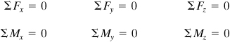
Consider a body in equilibrium subject to a system of external forces, as shown in Fig. 1.1a. Under the action of these forces, internal forces are developed within the body. To examine the latter at some interior point Q, we use an imaginary plane to cut the body at a section a–a through Q, dividing the body into two parts. As the forces acting on the entire body are in equilibrium, the forces acting on one part alone must be in equilibrium: this requires the presence of forces on plane a–a. These internal forces, applied to both parts, are distributed continuously over the cut surface. This process, referred to as the method of sections (Fig. 1.1), is relied on as a first step in solving all problems involving the investigation of internal forces.
Figure 1.1. Method of sections: (a) Sectioning of a loaded body; (b) free body with external and internal forces; (c) enlarged area ΔA with components of the force ΔF.
A free-body diagram is simply a sketch of a body with all the appropriate forces, both known and unknown, acting on it. Figure 1.1b shows such a plot of the isolated left part of the body. An element of area ΔA, located at point Q on the cut surface, is acted on by force ΔF. Let the origin of coordinates be placed at point Q, with x normal and y, z tangent to ΔA. In general, ΔF does not lie along x, y, or z.
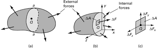
Decomposing ΔF into components parallel to x, y, and z (Fig. 1.1c), we define the normal stress σx and the shearing stresses τxy and τxz:
(1.5)
These definitions provide the stress components at a point Q to which the area ΔA is reduced in the limit. Clearly, the expression ΔA → 0 depends on the idealization discussed in Section 1.1. Our consideration is with the average stress on areas, which, while small as compared with the size of the body, is large compared with interatomic distances in the solid. Stress is thus defined adequately for engineering purposes. As shown in Eq. (1.5), the intensity of force perpendicular, or normal, to the surface is termed the normal stress at a point, while the intensity of force parallel to the surface is the shearing stress at a point.
The values obtained in the limiting process of Eq. (1.5) differ from point to point on the surface as ΔF varies. The stress components depend not only on ΔF, however, but also on the orientation of the plane on which it acts at point Q. Even at a given point, therefore, the stresses will differ as different planes are considered. The complete description of stress at a point thus requires the specification of the stress on all planes passing through the point.
Because the stress (σ or τ) is obtained by dividing the force by area, it has units of force per unit area. In SI units, stress is measured in newtons per square meter (N/m2), or pascals (Pa). As the pascal is a very small quantity, the megapascal (MPa) is commonly used. When U.S. Customary System units are used, stress is expressed in pounds per square inch (psi) or kips per square inch (ksi).
It is verified in Section 1.12 that in order to enable the determination of the stresses on an infinite number of planes passing through a point Q, thus defining the stresses at that point, we need only specify the stress components on three mutually perpendicular planes passing through the point. These three planes, perpendicular to the coordinate axes, contain three hidden sides of an infinitesimal cube (Fig. 1.2). We emphasize that when we move from point Q to point Q′ the values of stress will, in general, change. Also, body forces can exist. However, these cases are not discussed here (see Sec. 1.8), as we are now merely interested in establishing the terminology necessary to specify a stress component.
Figure 1.2. Element subjected to three-dimensional stress. All stresses have positive sense.
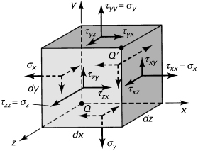
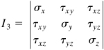
The general case of a three-dimensional state of stress is shown in Fig. 1.2. Consider the stresses to be identical at points Q and Q′ and uniformly distributed on each face, represented by a single vector acting at the center of each face. In accordance with the foregoing, a total of nine scalar stress components defines the state of stress at a point. The stress components can be assembled in the following matrix form, wherein each row represents the group of stresses acting on a plane passing through Q(x, y, z):
(1.6)
We note that in indicial notation (refer to Sec. 1.17), a stress component is written as τij, where the subscripts i and j each assume the values of x, y, and z as required by the foregoing equation. The double subscript notation is interpreted as follows: The first subscript indicates the direction of a normal to the plane or face on which the stress component acts; the second subscript relates to the direction of the stress itself. Repetitive subscripts are avoided in this text, so the normal stresses τxx, τyy, and τzz are designated σx, σy, and σz, as indicated in Eq. (1.6). A face or plane is usually identified by the axis normal to it; for example, the x faces are perpendicular to the x axis.
Sign Convention
Referring again to Fig. 1.2, we observe that both stresses labeled τyx tend to twist the element in a clockwise direction. It would be convenient, therefore, if a sign convention were adopted under which these stresses carried the same sign. Applying a convention relying solely on the coordinate direction of the stresses would clearly not produce the desired result, inasmuch as the τyx stress acting on the upper surface is directed in the positive x direction, while τyx acting on the lower surface is directed in the negative x direction. The following sign convention, which applies to both normal and shear stresses, is related to the deformational influence of a stress and is based on the relationship between the direction of an outward normal drawn to a particular surface and the directions of the stress components on the same surface.
When both the outer normal and the stress component face in a positive direction relative to the coordinate axes, the stress is positive. When both the outer normal and the stress component face in a negative direction relative to the coordinate axes, the stress is positive. When the normal points in a positive direction while the stress points in a negative direction (or vice versa), the stress is negative. In accordance with this sign convention, tensile stresses are always positive and compressive stresses always negative. Figure 1.2 depicts a system of positive normal and shear stresses.
Equality of Shearing Stresses
We now examine properties of shearing stress by studying the equilibrium of forces (see Sec. 1.4) acting on the cubic element shown in Fig. 1.2. As the stresses acting on opposite faces (which are of equal area) are equal in magnitude but opposite in direction, translational equilibrium in all directions is assured; that is, ΣFx = 0, ΣFy = 0, and ΣFz = 0. Rotational equilibrium is established by taking moments of the x-, y-, and z-directed forces about point Q, for example. From ΣMz = 0,
(–τxy dy dz)dx + (τyx dx dz)dy = 0
Simplifying,
(1.7a)
Likewise, from ΣMy = 0 and ΣMx = 0, we have
(1.7b)
Hence, the subscripts for the shearing stresses are commutative, and the stress tensor is symmetric. This means that shearing stresses on mutually perpendicular planes of the element are equal. Therefore, no distinction will hereafter be made between the stress components τxy and τyx, τxz and τzx, or τyz and τzy. In Section 1.8, it is shown rigorously that the foregoing is valid even when stress components vary from one point to another.
Some Special Cases of Stress
Under particular circumstances, the general state of stress (Fig. 1.2) reduces to simpler stress states, as briefly described here. These stresses, which are commonly encountered in practice, are given detailed consideration throughout the text.
a. Triaxial Stress. We shall observe in Section 1.13 that an element subjected to only stresses σ1, σ2, and σ3 acting in mutually perpendicular directions is said to be in a state of triaxial stress. Such a state of stress can be written as

(a)
The absence of shearing stresses indicates that the preceding stresses are the principal stresses for the element. A special case of triaxial stress, known as spherical or dilatational stress, occurs if all principal stresses are equal (see Sec. 1.14). Equal triaxial tension is sometimes called hydrostatic tension. An example of equal triaxial compression is found in a small element of liquid under static pressure.
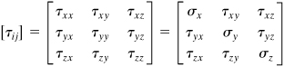
b. Two-Dimensional or Plane Stress. In this case, only the x and y faces of the element are subjected to stress, and all the stresses act parallel to the x and y axes, as shown in Fig. 1.3a. The plane stress matrix is written
(1.8)
Figure 1.3. (a) Element in plane stress; (b) two-dimensional presentation of plane stress; (c) element in pure shear.
Although the three-dimensional nature of the element under stress should not be forgotten, for the sake of convenience we usually draw only a two-dimensional view of the plane stress element (Fig. 1.3b). When only two normal stresses are present, the state of stress is called biaxial. These stresses occur in thin plates stressed in two mutually perpendicular directions.
c. Pure Shear. In this case, the element is subjected to plane shearing stresses only, for example, τxy and τyx (Fig. 1.3c). Typical pure shear occurs over the cross sections and on longitudinal planes of a circular shaft subjected to torsion.
d. Uniaxial Stress. When normal stresses act along one direction only, the one-dimensional state of stress is referred to as a uniaxial tension or compression.
1.6 Internal Force-Resultant and Stress Relations
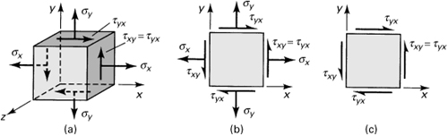
Distributed forces within a load-carrying member can be represented by a statically equivalent system consisting of a force and a moment vector acting at any arbitrary point (usually the centroid) of a section. These internal force resultants, also called stress resultants, exposed by an imaginary cutting plane containing the point through the member, are usually resolved into components normal and tangent to the cut section (Fig. 1.4). The sense of moments follows the right-hand screw rule, often represented by double-headed vectors, as shown in the figure. Each component can be associated with one of four modes of force transmission:
1. The axial force P or N tends to lengthen or shorten the member.
2. The shear forces Vy and Vz tend to shear one part of the member relative to the adjacent part and are often designated by the letter V.
3. The torque or twisting moment T is responsible for twisting the member.
4. The bending moments My and Mz cause the member to bend and are often identified by the letter M.
Figure 1.4. Positive forces and moments on a cut section of a body and components of the force dF on an infinitesimal area dA.
A member may be subject to any or all of the modes simultaneously. Note that the same sign convention is used for the force and moment components that is used for stress; a positive force (or moment) component acts on the positive face in the positive coordinate direction or on a negative face in the negative coordinate direction.
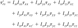
A typical infinitesimal area dA of the cut section shown in Fig. 1.4 is acted on by the components of an arbitrarily directed force dF, expressed using Eq. (1.5) as dFx = σx dA, dFy = τxy dA, and dFz = τxz dA. Clearly, the stress components on the cut section cause the internal force resultants on that section. Thus, the incremental forces are summed in the x, y, and z directions to give
(1.9a)
In a like manner, the sums of the moments of the same forces about the x, y, and z axes lead to
(1.9b)
where the integrations proceed over area A of the cut section. Equations (1.9) represent the relations between the internal force resultants and the stresses. In the next paragraph, we illustrate the fundamental concept of stress and observe how Eqs. (1.9) connect internal force resultants and the state of stress in a specific case.
Consider a homogeneous prismatic bar loaded by axial forces P at the ends (Fig. 1.5a). A prismatic bar is a straight member having constant cross-sectional area throughout its length. To obtain an expression for the normal stress, we make an imaginary cut (section a–a) through the member at right angles to its axis. A free-body diagram of the isolated part is shown in Fig. 1.5b, wherein the stress is substituted on the cut section as a replacement for the effect of the removed part. Equilibrium of axial forces requires that P = ∫ σx dA or P = Aσx. The normal stress is therefore
(1.10)
Figure 1.5. (a) Prismatic bar in tension; (b) Stress distribution across cross section.
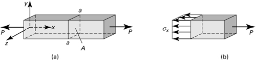
where A is the cross-sectional area of the bar. Because Vy, Vz, and T all are equal to zero, the second and third of Eqs. (1.9a) and the first of Eqs. (1.9b) are satisfied by τxy = τxz = 0. Also, My = Mz = 0 in Eqs. (1.9b) requires only that σx be symmetrically distributed about the y and z axes, as depicted in Fig. 1.5b. When the member is being extended as in the figure, the resulting stress is a uniaxial tensile stress; if the direction of forces were reversed, the bar would be in compression under uniaxial compressive stress. In the latter case, Eq. (1.10) is applicable only to chunky or short members owing to other effects that take place in longer members.*
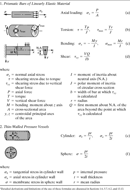
Similarly, application of Eqs. (1.9) to torsion members, beams, plates, and shells is presented as the subject unfolds, following the derivation of stress–strain relations and examination of the geometric behavior of a particular member. Applying the method of mechanics of materials, we develop other elementary formulas for stress and deformation. These, also called the basic formulas of mechanics of materials, are often used and extended for application to more complex problems in advanced mechanics of materials and the theory of elasticity. For reference purposes to preliminary discussions, Table 1.1 lists some commonly encountered cases. Note that in thin-walled vessels (r/t ≤ 10) there is often no distinction made between the inner and outer radii because they are nearly equal. In mechanics of materials, r denotes the inner radius. However, the more accurate shell theory (Sec. 13.11) is based on the average radius, which we use throughout this text. Each equation presented in the table describes a state of stress associated with a single force, torque, moment component, or pressure at a section of a typical homogeneous and elastic structural member [Ref. 1.7]. When a member is acted on simultaneously by two or more load types, causing various internal force resultants on a section, it is assumed that each load produces the stress as if it were the only load acting on the member. The final or combined stress is then determined by superposition of the several states of stress, as discussed in Section 2.2.
Table 1.1. Commonly Used Elementary Formulas for Stressa
The mechanics of materials theory is based on the simplifying assumptions related to the pattern of deformation so that the strain distributions for a cross section of the member can be determined. It is a basic assumption that plane sections before loading remain plane after loading. The assumption can be shown to be exact for axially loaded prismatic bars, for prismatic circular torsion members, and for prismatic beams subjected to pure bending. The assumption is approximate for other beam situations. However, it is emphasized that there is an extraordinarily large variety of cases in which applications of the basic formulas of mechanics of materials lead to useful results. In this text we hope to provide greater insight into the meaning and limitations of stress analysis by solving problems using both the elementary and exact methods of analysis.
1.7 Stresses on Inclined Sections
The stresses in bars, shafts, beams, and other structural members can be obtained by using the basic formulas, such as those listed in Table 1.1. The values found by these equations are for stresses that occur on cross sections of the members. Recall that all of the formulas for stress are limited to isotropic, homogeneous, and elastic materials that behave linearly. This section deals with the states of stress at points located on inclined sections or planes under axial loading. As before, we use stress elements to represent the state of stress at a point in a member. However, we now wish to find normal and shear stresses acting on the sides of an element in any direction.
The directional nature of more general states of stress and finding maximum and minimum values of stress are discussed in Sections 1.10 and 1.13. Usually, the failure of a member may be brought about by a certain magnitude of stress in a certain direction. For proper design, it is necessary to determine where and in what direction the largest stress occurs. The equations derived and the graphical technique introduced here and in the sections to follow are helpful in analyzing the stress at a point under various types of loading. Note that the transformation equations for stress are developed on the basis of equilibrium conditions only and do not depend on material properties or on the geometry of deformation.
Axially Loaded Members
We now consider the stresses on an inclined plane a–a of the bar in uniaxial tension shown in Fig. 1.6a, where the normal x′ to the plane forms an angle θ with the axial direction. On an isolated part of the bar to the left of section a–a, the resultant P may be resolved into two components: the normal force Px′ = P cos θ and the shear force Py′ = –P sin θ, as indicated in Fig. 1.6b. Thus, the normal and shearing stresses, uniformly distributed over the area Ax′ = A/cos θ of the inclined plane (Fig. 1.6c), are given by
(1.11a)
(1.11b)
Figure 1.6. (a) Prismatic bar in tension; (b, c) side views of a part cut from the bar.
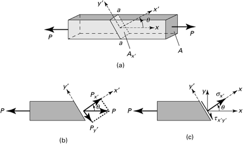
where σx = P/A. The negative sign in Eq. (1.11b) agrees with the sign convention for shearing stresses described in Section 1.5. The foregoing process of determining the stress in proceeding from one set of coordinate axes to another is called stress transformation.
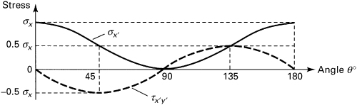
Equations (1.11) indicate how the stresses vary as the inclined plane is cut at various angles. As expected, σx′ is a maximum (σmax) when θ is 0° or 180°, and τx′y′ is maximum (τmax) when θ is 45° or 135°. Also, ![]() . The maximum stresses are thus
. The maximum stresses are thus
(1.12)
Observe that the normal stress is either maximum or a minimum on planes for which the shearing stress is zero.
Figure 1.7 shows the manner in which the stresses vary as the section is cut at angles varying from θ = 0° to 180°. Clearly, when θ > 90°, the sign of τx′y′ in Eq. (1.11b) changes; the shearing stress changes sense. However, the magnitude of the shearing stress for any angle θ determined from Eq. (1.11b) is equal to that for θ + 90°. This agrees with the general conclusion reached in the preceding section: shearing stresses on mutually perpendicular planes must be equal.
Figure 1.7. Example 1.1. Variation of stress at a point with the inclined section in the bar shown in Fig. 1.6a.
We note that Eqs. (1.11) can also be used for uniaxial compression by assigning to P a negative value. The sense of each stress direction is then reversed in Fig. 1.6c.
Example 1.1. State of Stress in a Tensile Bar
Compute the stresses on the inclined plane with θ = 35° for a prismatic bar of a cross-sectional area 800 mm2, subjected to a tensile load of 60 kN (Fig. 1.6a). Then determine the state of stress for θ = 35° by calculating the stresses on an adjoining face of a stress element. Sketch the stress configuration.
Solution
The normal stress on a cross section is
![]()
Introducing this value in Eqs. (1.11) and using θ = 35°, we have
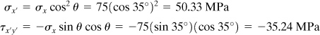
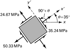
The normal and shearing stresses acting on the adjoining y′ face are, respectively, 24.67 MPa and 35.24 MPa, as calculated from Eqs. (1.11) by substituting the angle θ + 90° = 125°. The values of σx′ and τx′y′ are the same on opposite sides of the element. On the basis of the established sign convention for stress, the required sketch is shown in Fig. 1.8.
Figure 1.8. Example 1.1. Stress element for θ = 35°.
1.8 Variation of Stress within a Body
As pointed out in Section 1.5, the components of stress generally vary from point to point in a stressed body. These variations are governed by the conditions of equilibrium of statics. Fulfillment of these conditions establishes certain relationships, known as the differential equations of equilibrium, which involve the derivatives of the stress components.
Consider a thin element of sides dx and dy (Fig. 1.9), and assume that σx, σy, τxy, and τyx are functions of x, y but do not vary throughout the thickness (are independent of z) and that the other stress components are zero. Also assume that the x and y components of the body forces per unit volume, Fx and Fy, are independent of z and that the z component of the body force Fz = 0. This combination of stresses, satisfying the conditions described, is the plane stress. Note that because the element is very small, for the sake of simplicity, the stress components may be considered to be distributed uniformly over each face. In the figure they are shown by a single vector representing the mean values applied at the center of each face.
Figure 1.9. Element with stresses and body forces.
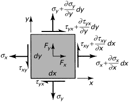
As we move from one point to another, for example, from the lower-left corner to the upper-right corner of the element, one stress component, say σx, acting on the negative x face, changes in value on the positive x face. The stresses σy, τxy, and τyx similarly change. The variation of stress with position may be expressed by a truncated Taylor’s expansion:
(a)
The partial derivative is used because σx is a function of x and y. Treating all the components similarly, the state of stress shown in Fig. 1.9 is obtained.
We consider now the equilibrium of an element of unit thickness, taking moments of force about the lower-left corner. Thus, ΣMz = 0 yields
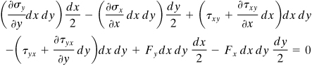
Neglecting the triple products involving dx and dy, this reduces to τxy = τyx. In a like manner, it may be shown that τyz = τzy and τxz = τzx, as already obtained in Section 1.5. From the equilibrium of x forces, ΣFx = 0, we have
(b)
Upon simplification, Eq. (b) becomes
(c)
Inasmuch as dx dy is nonzero, the quantity in the parentheses must vanish. A similar expression is written to describe the equilibrium of y forces. The x and y equations yield the following differential equations of equilibrium for two-dimensional stress:
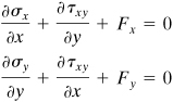
(1.13)
The differential equations of equilibrium for the case of three-dimensional stress may be generalized from the preceding expressions as follows:
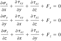
(1.14)
A succinct representation of these expressions, on the basis of the range and summation conventions (Sec. 1.17), may be written as
(1.15a)
where xx = x, xy = y, and xz = z. The repeated subscript is j, indicating summation. The unrepeated subscript is i. Here i is termed the free index, and j, the dummy index.
If in the foregoing expression the symbol ∂/∂x is replaced by a comma, we have
(1.15b)
where the subscript after the comma denotes the coordinate with respect to which differentiation is performed. If no body forces exist, Eq. (1.15b) reduces to τij,j = 0, indicating that the sum of the three stress derivatives is zero. As the two equilibrium relations of Eqs. (1.13) contain three unknowns (σx, σy, τxy) and the three expressions of Eqs. (1.14) involve the six unknown stress components, problems in stress analysis are internally statically indeterminate.
In a number of practical applications, the weight of the member is the only body force. If we take the y axis as upward and designate by ρ the mass density per unit volume of the member and by g, the gravitational acceleration, then Fx = Fz = 0 and Fy = –ρg in Eqs. (1.13) and (1.14). The resultant of this force over the volume of the member is usually so small compared with the surface forces that it can be ignored, as stated in Section 1.1. However, in dynamic systems, the stresses caused by body forces may far exceed those associated with surface forces so as to be the principal influence on the stress field.*
Application of Eqs. (1.13) and (1.14) to a variety of loaded members is presented in sections employing the approach of the theory of elasticity, beginning with Chapter 3. The following sample problem shows the pattern of the body force distribution for an arbitrary state of stress in equilibrium.
Example 1.2. The Body Forces in a Structure
The stress field within an elastic structural member is expressed as follows:
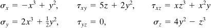
(d)
Determine the body force distribution required for equilibrium.
Solution
Substitution of the given stresses into Eq. (1.14) yields
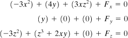
The body force distribution, as obtained from these expressions, is therefore
(e)
The state of stress and body force at any specific point within the member may be obtained by substituting the specific values of x, y, and z into Eqs. (d) and (e), respectively.
1.9 Plane-Stress Transformation
A two-dimensional state of stress exists when the stresses and body forces are independent of one of the coordinates, here taken as z. Such a state is described by stresses σx, σy, and τxy and the x and y body forces. Two-dimensional problems are of two classes: plane stress and plane strain. In the case of plane stress, as described in the previous section, the stresses σz, τxz, and τyz, and the z-directed body forces are assumed to be zero. The condition that occurs in a thin plate subjected to loading uniformly distributed over the thickness and parallel to the plane of the plate typifies the state of plane stress (Fig. 1.10). In the case of plane strain, the stresses τxz and τyz and the body force Fz are likewise taken to be zero, but σz does not vanish* and can be determined from stresses σx and σy.
Figure 1.10. Thin Plate in-plane loads.
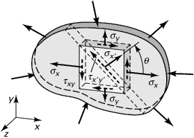
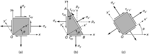
We shall now determine the equations for transformation of the stress components σx, σy, and τxy at any point of a body represented by an infinitesimal element, isolated from the plate illustrated in Fig. 1.10. The z-directed normal stress σz, even if it is nonzero, need not be considered here. In the following derivations, the angle θ locating the x′ axis is assumed positive when measured from the x axis in a counterclockwise direction. Note that, according to our sign convention (see Sec. 1.5), the stresses are indicated as positive values.
Consider an infinitesimal wedge cut from the loaded body shown in Fig. 1.11a, b. It is required to determine the stresses σx′ and τx′y′, which refer to axes x′, y′ making an angle θ with axes x, y, as shown in the figure. Let side AB be normal to the x′ axis. Note that in accordance with the sign convention, σx′ and τx′y′ are positive stresses, as shown in the figure. If the area of side AB is taken as unity, then sides QA and QB have area cos θ and sin θ, respectively.
Figure 1.11. Elements in plane stress.
Equilibrium of forces in the x and y directions requires that
(1.16)
where px and py are the components of stress resultant acting on AB in the x and y directions, respectively. The normal and shear stresses on the x′ plane (AB plane) are obtained by projecting px and py in the x′ and y′ directions:
(a)
From the foregoing it is clear that ![]() . Upon substitution of the stress resultants from Eq. (1.16), Eqs. (a) become
. Upon substitution of the stress resultants from Eq. (1.16), Eqs. (a) become
(1.17a)
(1.17b)
Note that the normal stress σy′ acting on the y′ face of an inclined element (Fig. 1.11c) may readily be obtained by substituting θ + π/2 for θ in the expression for σx′. In so doing, we have
(1.17c)
Equations (1.17) can be converted to a useful form by introducing the following trigonometric identities:
![]()
The transformation equations for plane stress now become
(1.18a)
(1.18b)
(1.18c)
The foregoing expressions permit the computation of stresses acting on all possible planes AB (the state of stress at a point) provided that three stress components on a set of orthogonal faces are known.
Stress tensor. It is important to note that addition of Eqs. (1.17a) and (1.17c) gives the relationships
σx + σy = σx′ + σy′ = constant
In words then, the sum of the normal stresses on two perpendicular planes is invariant—that is, independent of θ. This conclusion is also valid in the case of a three-dimensional state of stress, as shown in Section 1.13. In mathematical terms, the stress whose components transform in the preceding way by rotation of axes is termed tensor. Some examples of other quantities are strain and moment of inertia. The similarities between the transformation equations for these quantities are observed in Sections 2.5 and C.4. Mohr’s circle (Sec. 1.11) is a graphical representation of a stress tensor transformation.
Polar Representations of State of Plane Stress
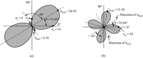
Consider, for example, the possible states of stress corresponding to σx = 14 MPa, σy = 4 MPa, and τxy = 10 MPa. Substituting these values into Eq. (1.18) and permitting θ to vary from 0° to 360° yields the data upon which the curves shown in Fig. 1.12 are based. The plots shown, called stress trajectories, are polar representations: σx′ versus θ (Fig. 1.12a) and τx′y′ versus θ (Fig. 1.12b). It is observed that the direction of each maximum shear stress bisects the angle between the maximum and minimum normal stresses. Note that the normal stress is either a maximum or a minimum on planes at θ = 31.66° and θ = 31.66° + 90°, respectively, for which the shearing stress is zero. The conclusions drawn from this example are valid for any two-dimensional (or three-dimensional) state of stress and are observed in the sections to follow.
Figure 1.12. Polar representations of σx′ and τx′y′ (in megapascals) versus θ.
Cartesian Representation of State of Plane Stress
Now let us examine a two-dimensional condition of stress at a point in a loaded machine component on an element illustrated in Fig. 1.13a. Introducing the given values into the first two of Eqs. (1.18), gives
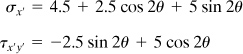
Figure 1.13. Graph of normal stress σx′ and shearing stress τx′y′ with angle θ (for θ ≤ 180°).
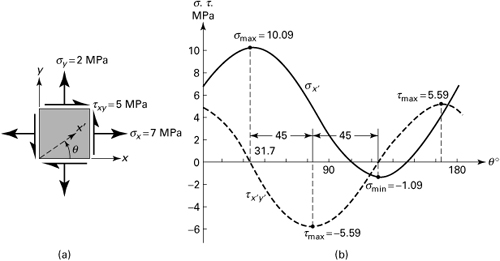
In the foregoing, permitting θ to vary from 0° to 180° in increments of 15° leads to the data from which the graphs illustrated in Fig. 1.13b are obtained [Ref. 1.7]. This Cartesian representation demonstrates the variation of the normal and shearing stresses versus θ ≤ 180°. Observe that the direction of maximum (and minimum) shear stress bisects the angle between the maximum and minimum normal stresses. Moreover, the normal stress is either a maximum or a minimum on planes θ = 31.7° and θ = 31.7° + 90°, respectively, for which the shear stress is zero. Note as a check that σx + σy = σmax + σmin = 9 MPa, as expected.
The conclusions drawn from the foregoing polar and Cartesian representations are valid for any state of stress, as will be seen in the next section. A more convenient approach to the graphical transformation for stress is considered in Sections 1.11 and 1.15. The manner in which the three-dimensional normal and shearing stresses vary is discussed in Sections 1.12 through 1.14.
1.10 Principal Stresses and Maximum In-Plane Shear Stress
The transformation equations for two-dimensional stress indicate that the normal stress σx′ and shearing stress τx′y′ vary continuously as the axes are rotated through the angle θ. To ascertain the orientation of x′y′ corresponding to maximum or minimum σx′, the necessary condition dσx′/dθ = 0 is applied to Eq. (1.18a). In so doing, we have
(a)
This yields
(1.19)
Inasmuch as tan 2θ = tan(π + 2θ), two directions, mutually perpendicular, are found to satisfy Eq. (1.19). These are the principal directions, along which the principal or maximum and minimum normal stresses act. Two values of θp, corresponding to the σ1 and σ2 planes, are represented by ![]() and
and ![]() , respectively.
, respectively.
When Eq. (1.18b) is compared with Eq. (a), it becomes clear that τx′y′ = 0 on a principal plane. A principal plane is thus a plane of zero shear. The principal stresses are determined by substituting Eq. (1.19) into Eq. (1.18a):
(1.20)
Note that the algebraically larger stress given here is the maximum principal stress, denoted by σ1. The minimum principal stress is represented by σ2. It is necessary to substitute one of the values θp into Eq. (1.18a) to determine which of the two corresponds to σ1.
Similarly, employing the preceding approach and Eq. (1.18b), we determine the planes of maximum shearing stress. Thus, setting dτx′y′/dθ = 0, we now have (σx – σy)cos 2θ + 2τxy sin 2θ = 0 or
(1.21)
The foregoing expression defines two values of θs that are 90° apart. These directions may again be denoted by attaching a prime or a double prime notation to θs. Comparing Eqs. (1.19) and (1.21), we also observe that the planes of maximum shearing stress are inclined at 45° with respect to the planes of principal stress. Now, from Eqs. (1.21) and (1.18b), we obtain the extreme values of shearing stress as follows:
(1.22)
Here the largest shearing stress, regardless of sign, is referred to as the maximum shearing stress, designated τmax. Normal stresses acting on the planes of maximum shearing stress can be determined by substituting the values of 2θs from Eq. (1.21) into Eqs. (1.18a) and (1.18c):
(1.23)
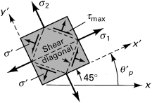
The results are illustrated in Fig. 1.14. Note that the diagonal of a stress element toward which the shearing stresses act is called the shear diagonal. The shear diagonal of the element on which the maximum shearing stresses act lies in the direction of the algebraically larger principal stress as shown in the figure. This assists in predicting the proper direction of the maximum shearing stress.
Figure 1.14. Planes of principal and maximum shearing stresses.
1.11 Mohr’s Circle for Two-Dimensional Stress
A graphical technique, predicated on Eq. (1.18), permits the rapid transformation of stress from one plane to another and leads also to the determination of the maximum normal and shear stresses. In this approach, Eqs. (1.18) are depicted by a stress circle, called Mohr’s circle.* In the Mohr representation, the normal stresses obey the sign convention of Section 1.5. However, for the purposes only of constructing and reading values of stress from Mohr’s circle, the sign convention for shear stress is as follows: If the shearing stresses on opposite faces of an element would produce shearing forces that result in a clockwise couple, as shown in Fig. 1.15c, these stresses are regarded as positive. Accordingly, the shearing stresses on the y faces of the element in Fig. 1.15a are taken as positive (as before), but those on the x faces are now negative.
Figure 1.15. (a) Stress element; (b) Mohr’s circle of stress; (c) interpretation of positive shearing stresses.
Given σx, σy, and τxy with algebraic sign in accordance with the foregoing sign convention, the procedure for obtaining Mohr’s circle (Fig. 1.15b) is as follows:
1. Establish a rectangular coordinate system, indicating +τ and +σ. Both stress scales must be identical.
2. Locate the center C of the circle on the horizontal axis a distance ![]() from the origin.
from the origin.
3. Locate point A by coordinates σx and –τxy. These stresses may correspond to any face of an element such as in Fig. 1.15a. It is usual to specify the stresses on the positive x face, however.
4. Draw a circle with center at C and of radius equal to CA.
5. Draw line AB through C.
The angles on the circle are measured in the same direction as θ is measured in Fig. 1.15a. An angle of 2θ on the circle corresponds to an angle of θ on the element. The state of stress associated with the original x and y planes corresponds to points A and B on the circle, respectively. Points lying on diameters other than AB, such as A′ and B′, define states of stress with respect to any other set of x′ and y′ planes rotated relative to the original set through an angle θ.
It is clear that points A1 and B1 on the circle locate the principal stresses and provide their magnitudes as defined by Eqs. (1.19) and (1.20), while D and E represent the maximum shearing stresses, defined by Eqs. (1.21) and (1.22). The radius of the circle is
(a)
where
![]()
Thus, the radius equals the magnitude of the maximum shearing stress. Mohr’s circle shows that the planes of maximum shear are always located at 45° from planes of principal stress, as already indicated in Fig. 1.14. The use of Mohr’s circle is illustrated in the first two of the following examples.
Example 1.3. Principal Stresses in a Member
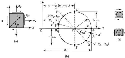
At a point in the structural member, the stresses are represented as in Fig. 1.16a. Employ Mohr’s circle to determine (a) the magnitude and orientation of the principal stresses and (b) the magnitude and orientation of the maximum shearing stresses and associated normal stresses. In each case, show the results on a properly oriented element; represent the stress tensor in matrix form.
Figure 1.16. Example 1.3. (a) Element in plane stress; (b) Mohr’s circle of stress; (c) principal stresses; (d) maximum shear stress.
Solution
Mohr’s circle, constructed in accordance with the procedure outlined, is shown in Fig. 1.16b. The center of the circle is at (40 + 80)/2 = 60 MPa on the σ axis.
a. The principal stresses are represented by points A1 and B1 Hence, the maximum and minimum principal stresses, referring to the circle, are
![]()
or
![]()
The planes on which the principal stresses act are given by
![]()
Hence
![]()
Mohr’s circle clearly indicates that ![]() locates the σ1 plane. The results may readily be checked by substituting the two values of θp into Eq. (1.18a). The state of principal stress is shown in Fig. 1.16c.
locates the σ1 plane. The results may readily be checked by substituting the two values of θp into Eq. (1.18a). The state of principal stress is shown in Fig. 1.16c.
b. The maximum shearing stresses are given by points D and E. Thus,
![]()
It is seen that (σ1 – σ2)/2 yields the same result. The planes on which these stresses act are represented by
![]()
As Mohr’s circle indicates, the positive maximum shearing stress acts on a plane whose normal x′ makes an angle ![]() with the normal to the original plane (x plane). Thus, +τmax on two opposite x′ faces of the element will be directed so that a clockwise couple results. The normal stresses acting on maximum shear planes are represented by OC, σ′ = 60 MPa on each face. The state of maximum shearing stress is shown in Fig. 1.16d. The direction of the τmax’s may also be readily predicted by recalling that they act toward the shear diagonal. We note that, according to the general sign convention (Sec. 1.5), the shearing stress acting on the x′ plane in Fig. 1.16d is negative. As a check, if
with the normal to the original plane (x plane). Thus, +τmax on two opposite x′ faces of the element will be directed so that a clockwise couple results. The normal stresses acting on maximum shear planes are represented by OC, σ′ = 60 MPa on each face. The state of maximum shearing stress is shown in Fig. 1.16d. The direction of the τmax’s may also be readily predicted by recalling that they act toward the shear diagonal. We note that, according to the general sign convention (Sec. 1.5), the shearing stress acting on the x′ plane in Fig. 1.16d is negative. As a check, if ![]() and the given initial data are substituted into Eq. (1.18b), we obtain τx′y′ = –36.05 MPa, as already found.
and the given initial data are substituted into Eq. (1.18b), we obtain τx′y′ = –36.05 MPa, as already found.
We may now describe the state of stress at the point in the following matrix forms:
![]()
These three representations, associated with the θ = 0°, θ = 28.15°, and θ = 73.15° planes passing through the point, are equivalent.
Note that if we assume σz = 0 in this example, a much higher shearing stress is obtained in the planes bisecting the x′ and z planes (Problem 1.56). Thus, three-dimensional analysis, Section 1.15, should be considered for determining the true maximum shearing stress at a point.
Example 1.4. Stresses in a Frame
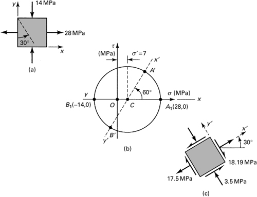
The stresses acting on an element of a loaded frame are shown in Fig. 1.17a. Apply Mohr’s circle to determine the normal and shear stresses acting on a plane defined by θ = 30°.
Figure 1.17. Example 1.4. (a) Element in biaxial stresses; (b) Mohr’s circle of stress; (c) stress element for θ = 30°.
Solution
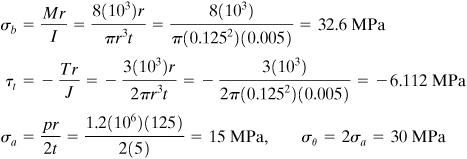
Mohr’s circle of Fig. 1.17b describes the state of stress given in Fig. 1.17a. Points A1 and B1 represent the stress components on the x and y faces, respectively. The radius of the circle is (14 + 28)/2 = 21. Corresponding to the 30° plane within the element, it is necessary to rotate through 60° counterclockwise on the circle to locate point A′. A 240° counterclockwise rotation locates point B′. Referring to the circle,
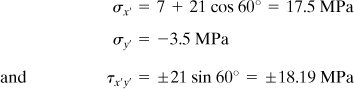
Figure 1.17c indicates the orientation of the stresses. The results can be checked by applying Eq. (1.18), using the initial data.
Example 1.5. Cylindrical Vessel Under Combined Loads
A thin-walled cylindrical pressure vessel of 250-mm diameter and 5-mm wall thickness is rigidly attached to a wall, forming a cantilever (Fig. 1.18a). Determine the maximum shearing stresses and the associated normal stresses at point A of the cylindrical wall. The following loads are applied: internal pressure p = 1.2 MPa, torque T = 3 kN · m, and direct force P = 20 kN. Show the results on a properly oriented element.
Figure 1.18. Example 1.5. Combined stresses in a thin-walled cylindrical pressure vessel: (a) side view; (b) free body of a segment; (c) and (d) element A (viewed from top).
Solution
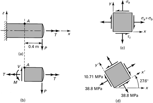
The internal force resultants on a transverse section through point A are found from the equilibrium conditions of the free-body diagram of Fig. 1.18b. They are V = 20 kN, M = 8 kN · m, and T = 3 kN · m. In Fig. 1.18c, the combined axial, tangential, and shearing stresses are shown acting on a small element at point A. These stresses are (Tables 1.1 and C.1)
We thus have σx = 47.6 MPa, σy = 30 MPa, and τxy = –6.112 MPa. Note that for element A, Q = 0; hence, the direct shearing stress τd = τxz = VQ/Ib = 0.
The maximum shearing stresses are from Eq. (1.22):
![]()
Equation (1.23) yields
![]()
To locate the maximum shear planes, we use Eq. (1.21):
![]()
Applying Eq. (1.18b) with the given data and 2θs = 55.2°, τx′y′ = –10.71 MPa. Hence, ![]() , and the stresses are shown in their proper directions in Fig. 1.18d.
, and the stresses are shown in their proper directions in Fig. 1.18d.
1.12 Three-Dimensional Stress Transformation
The physical elements studied are always three dimensional, and hence it is desirable to consider three planes and their associated stresses, as illustrated in Fig. 1.2. We note that equations governing the transformation of stress in the three-dimensional case may be obtained by the use of a similar approach to that used for the two-dimensional state of stress.
Consider a small tetrahedron isolated from a continuous medium (Fig. 1.19a), subject to a general state of stress. The body forces are taken to be negligible. In the figure, px, py, and pz are the Cartesian components of stress resultant p acting on oblique plane ABC. It is required to relate the stresses on the perpendicular planes intersecting at the origin to the normal and shear stresses on ABC.
Figure 1.19. Stress components on a tetrahedron.
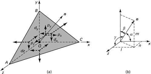
The orientation of plane ABC may be defined in terms of the angles between a unit normal n to the plane and the x, y, and z directions (Fig. 1.19b). The direction cosines associated with these angles are
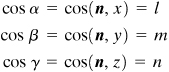
(1.24)
The three direction cosines for the n direction are related by
(1.25)
The area of the perpendicular plane QAB, QAC, QBC may now be expressed in terms of A, the area of ABC, and the direction cosines:
AQAB = Ax = A · i = A(li + mj + nk) · i = Al
The other two areas are similarly obtained. In so doing, we have altogether
(a)
Here i, j, and k are unit vectors in the x, y, and z directions, respectively.
Next, from the equilibrium of x, y, z-directed forces together with Eq. (a), we obtain, after canceling A,
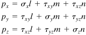
(1.26)
The stress resultant on A is thus determined on the basis of known stresses σx, σy, σz, τxy, τxz, and τyz and a knowledge of the orientation of A. In the limit as the sides of the tetrahedron approach zero, plane A contains point Q. It is thus demonstrated that the stress resultant at a point is specified. This in turn gives the stress components acting on any three mutually perpendicular planes passing through Q as shown next. Although perpendicular planes have been used there for convenience, these planes need not be perpendicular to define the stress at a point.
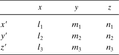
Consider now a Cartesian coordinate system x′, y′, z′, wherein x′ coincides with n and y′, z′ lie on an oblique plane. The x′ y′ z′ and xyz systems are related by the direction cosines: l1 = cos (x′, x), m1 = cos(x′, y), and so on. The notation corresponding to a complete set of direction cosines is shown in Table 1.2. The normal stress σx′ is found by projecting px, py, and pz in the x′ direction and adding
(1.27)
Table 1.2. Notation for Direction Cosines
Equations (1.26) and (1.27) are combined to yield
(1.28a)
Similarly, by projecting px, py, and pz in the y′ and z′ directions, we obtain, respectively,
(1.28b)
(1.28c)
Recalling that the stresses on three mutually perpendicular planes are required to specify the stress at a point (one of these planes being the oblique plane in question), the remaining components are found by considering those planes perpendicular to the oblique plane. For one such plane, n would now coincide with the y′ direction, and expressions for the stresses σy′, τy′x′, and τy′z′ would be derived. In a similar manner, the stresses σz′, τz′x′, and τz′y′ are determined when n coincides with the z′ direction. Owing to the symmetry of the stress tensor, only six of the nine stress components thus developed are unique. The remaining stress components are as follows:
(1.28d)
(1.28e)
(1.28f)
Equations (1.28) represent expressions transforming the quantities σx, σy, σz, τxy, τxz, and τyz which, as we have noted, completely define the state of stress. Quantities such as stress (and moment of inertia, Appendix C), which are subject to such transformations, are tensors of second rank (see Sec. 1.9).
The equations of transformation of the components of a stress tensor, in indicial notation, are represented by
(1.29a)
Alternatively,
(1.29b)
The repeated subscripts i and j imply the double summation in Eq. (1.29a), which, upon expansion, yields
(1.29c)
By assigning r, s = x, y, z and noting that τrs = τsr, the foregoing leads to the six expressions of Eq. (1.28).
It is interesting to note that, because x′, y′, and z′ are orthogonal, the nine direction cosines must satisfy trigonometric relations of the following form:
(1.30a)
and
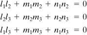
(1.30b)
From Table 1.2, observe that Eqs. (1.30a) are the sums of the squares of the cosines in each row, and Eqs. (1.30b) are the sums of the products of the adjacent cosines in any two rows.
1.13 Principal Stresses in Three Dimensions
For the three-dimensional case, it is now demonstrated that three planes of zero shear stress exist, that these planes are mutually perpendicular, and that on these planes the normal stresses have maximum or minimum values. As has been discussed, these normal stresses are referred to as principal stresses, usually denoted σ1, σ2, and σ3. The algebraically largest stress is represented by σ1, and the smallest by σ3: σ1 > σ2 > σ3.
We begin by again considering an oblique x′ plane. The normal stress acting on this plane is given by Eq. (1.28a):
(a)
The problem at hand is the determination of extreme or stationary values of σx′. To accomplish this, we examine the variation of σx′ relative to the direction cosines. Inasmuch as l, m, and n are not independent, but connected by l2 + m2 + n2 = 1, only l and m may be regarded as independent variables. Thus,
(b)
Differentiating Eq. (a) as indicated by Eqs. (b) in terms of the quantities in Eq. (1.26), we obtain
(c)
From n2 = 1 – l2 – m2, we have ∂n/∂l = –l/n and ∂n/∂m = –m/n. Introducing these into Eq. (c), the following relationships between the components of p and n are determined:
(d)
These proportionalities indicate that the stress resultant must be parallel to the unit normal and therefore contains no shear component. It is concluded that, on a plane for which σx′ has an extreme or principal value, a principal plane, the shearing stress vanishes.
It is now shown that three principal stresses and three principal planes exist. Denoting the principal stresses by σp, Eq. (d) may be written as
(e)
These expressions, together with Eq. (1.26), lead to
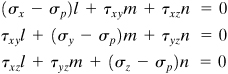
(1.31)
A nontrivial solution for the direction cosines requires that the characteristic determinant vanish:
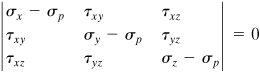
(1.32)
Expanding Eq. (1.32) leads to
(1.33)
where
(1.34a)
(1.34b)
(1.34c)
The three roots of the stress cubic equation (1.33) are the principal stresses, corresponding to which are three sets of direction cosines, which establish the relationship of the principal planes to the origin of the nonprincipal axes. The principal stresses are the characteristic values or eigenvalues of the stress tensor τij. Since the stress tensor is a symmetric tensor whose elements are all real, it has real eigenvalues. That is, the three principal stresses are real [Refs. 1.8 and 1.9]. The direction cosines l, m, and n are the eigenvectors of τij.
It is clear that the principal stresses are independent of the orientation of the original coordinate system. It follows from Eq. (1.33) that the coefficients I1, I2, and I3 must likewise be independent of x, y, and z, since otherwise the principal stresses would change. For example, we can demonstrate that adding the expressions for σx′, σy′, and σz′ given by Eq. (1.28) and making use of Eq. (1.30a) leads to I1 = σx′ + σy′ + σz′ = σx + σy + σz. Thus, the coefficients I1, I2, and I3 represent three invariants of the stress tensor in three dimensions or, briefly, the stress invariants. For plane stress, it is a simple matter to show that the following quantities are invariant (Prob. 1.27):
(1.35)
Equations (1.34) and (1.35) are particularly helpful in checking the results of a stress transformation, as illustrated in Example 1.7.
If now one of the principal stresses, say σ1 obtained from Eq. (1.33), is substituted into Eq. (1.31), the resulting expressions, together with l2 + m2 + n2 = 1, provide enough information to solve for the direction cosines, thus specifying the orientation of σ1 relative to the xyz system. The direction cosines of σ2 and σ3 are similarly obtained. A convenient way of determining the roots of the stress cubic equation and solving for the direction cosines is presented in Appendix B, where a related computer program is also included (see Table B.1).
Example 1.6. Three-Dimensional Stress in a Hub
A steel shaft is to be force fitted into a fixed-ended cast-iron hub. The shaft is subjected to a bending moment M, a torque T, and a vertical force P, Fig. 1.20a. Suppose that at a point Q in the hub, the stress field is as shown in Fig. 1.20b, represented by the matrix
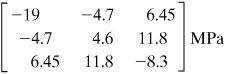
Figure 1.20. Example 1.6. (a) Hub-shaft assembly. (b) Element in three-dimensional stress.
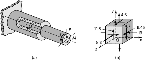
Determine the principal stresses and their orientation with respect to the original coordinate system.
Solution
Substituting the given stresses into Eq. (1.33) we obtain from Eqs. (B.2)
![]()
Successive introduction of these values into Eq. (1.31), together with Eq. (1.30a), or application of Eqs. (B.6) yields the direction cosines that define the orientation of the planes on which σ1, σ2, and σ3 act:
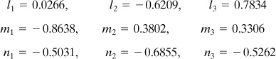
Note that the directions of the principal stresses are seldom required for purposes of predicting the behavior of structural members.
Example 1.7. Three-Dimensional Stress in a Machine Component
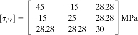
The stress tensor at a point in a machine element with respect to a Cartesian coordinate system is given by the following array:
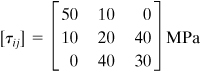
(f)
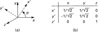
Determine the state of stress and I1, I2, and I3 for an x′, y′, z′ coordinate system defined by rotating x, y through an angle of θ = 45° counterclockwise about the z axis (Fig. 1.21a).
Figure 1.21. Example 1.7. Direction cosines for θ = 45°.
Solution
The direction cosines corresponding to the prescribed rotation of axes are given in Fig. 1.21b. Thus, through the use of Eq. (1.28) we obtain
(g)
It is seen that the arrays (f) and (g), when substituted into Eq. (1.34), both yield I1 = 100 MPa, I2 = 1400 (MPa)2, and I3 = –53,000 (MPa)3, and the invariance of I1, I2, and I3 under the orthogonal transformation is confirmed.
1.14 Normal and Shear Stresses on an Oblique Plane
A cubic element subjected to principal stresses σ1, σ2, and σ3 acting on mutually perpendicular principal planes is called in a state of triaxial stress (Fig. 1.22a). In the figure, the x, y, and z axes are parallel to the principal axes. Clearly, this stress condition is not the general case of three-dimensional stress, which was taken up in the last two sections. It is sometimes required to determine the shearing and normal stresses acting on an arbitrary oblique plane of a tetrahedron, as in Fig. 1.22b, given the principal stresses or triaxial stresses acting on perpendicular planes. In the figure, the x, y, and z axes are parallel to the principal axes. Denoting the direction cosines of plane ABC by l, m, and n, Eqs. (1.26) with σx = σ1, τxy = τxz = 0, and so on, reduce to
(a)
Figure 1.22. Elements in triaxial stress.
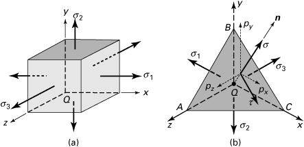
Referring to Fig. 1.22a and definitions (a), the stress resultant p is related to the principal stresses and the stress components on the oblique plane by the expression
(1.36)
The normal stress σ on this plane, from Eq. (1.28a), is found as
(1.37)
Substitution of this expression into Eq. (1.36) leads to
(1.38a)
or
(1.38b)
Expanding and using the expressions 1 – l2 = m2 + n2, 1 – n2 = l2 + m2, and so on, the following result is obtained for the shearing stress τ on the oblique plane:
(1.39)
This clearly indicates that if the principal stresses are all equal, the shear stress vanishes, regardless of the choices of the direction cosines.
For situations in which shear as well as normal stresses act on perpendicular planes (Fig. 1.22b), we have px, py, and pz defined by Eqs. (1.26). Then, Eq. (1.37) becomes
(1.40)
Hence,
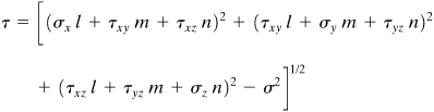
(1.41)
where σ is given by Eq. (1.40). Formulas (1.37) through (1.41) represent the simplified transformation expressions for the three-dimensional stress.
It is interesting to note that substitution of the direction cosines from Eqs. (a) into Eq. (1.25) leads to
(1.42)
which is a stress ellipsoid having its three semiaxes as the principal stresses (Fig. 1.23). This geometrical interpretation helps to explain the earlier conclusion that the principal stresses are the extreme values of the normal stress. In the event that σ1 = σ2 = σ3, a state of hydrostatic stress exists, and the stress ellipsoid becomes a sphere. In this case, note again that any three mutually perpendicular axes can be taken as the principal axes.
Figure 1.23. Stress ellipsoid.
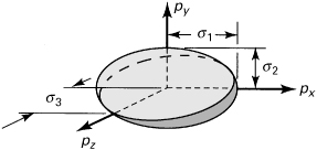
Octahedral Stresses
The stresses acting on an octahedral plane is represented by face ABC in Fig. 1.22b with QA = QB = QC. The normal to this oblique face thus has equal direction cosines relative to the principal axes. Since l2 + m2 + n2 = 1, we have
(b)
Plane ABC is clearly one of eight such faces of a regular octahedron (Fig. 1.24). Equations (1.39) and (b) are now applied to provide an expression for the octahedral shearing stress, which may be rearranged to the form
(1.43)
Figure 1.24. Stresses on an octahedron.
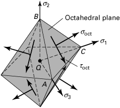
Through the use of Eqs. (1.37) and (b), we obtain the octahedral normal stress:
(1.44)
The normal stress acting on an octahedral plane is thus the average of the principal stresses, the mean stress. The orientations of σoct and τoct are indicated in Fig. 1.24. That the normal and shear stresses are the same for the eight planes is a powerful tool for failure analysis of ductile materials (see Sec. 4.8). Another useful form of Eq. (1.43) is developed in Section 2.15.
1.15 Mohr’s Circles in Three Dimensions
Consider a wedge shown in Fig. 1.25a, cut from the cubic element subjected to triaxial stresses (Fig. 1.22a). The only stresses on the inclined x′ face (parallel to the z axis) are the normal stress σx′ and the shear stress τx′y′ acting in the x′y′ plane. Inasmuch as the foregoing stresses are determined from force equilibrium equations in the x′y′ plane, they are independent of the stress σ3. Thus, the transformation equations of plane stress (Sec. 1.9) and Mohr’s circle can be employed to obtain the stresses σx′ and τx′y′. The foregoing conclusion is also valid for normal and shear stresses acting on inclined faces cut through the element parallel to the x and y axes.
Figure 1.25. Triaxial state of stress: (a) wedge; (b) planes of maximum shear stress.
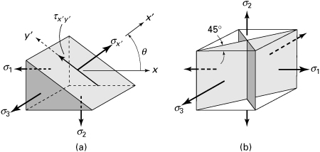
The stresses acting on elements oriented at various angles to the principal axes can be visualized with the aid of Mohr’s circle. The cubic element (Fig. 1.22a) viewed from three different directions is sketched in Figs. 1.26a to c. A Mohr’s circle is drawn corresponding to each projection of an element. The cluster of three circles represents Mohr’s circles for triaxial stress (Fig. 1.26d). The radii of the circles are equal to the maximum shear stresses, as indicated in the figure. The normal stresses acting on the planes of maximum shear stresses have the magnitudes given by the abscissa as of the centers of the circles.
Figure 1.26. (a–c) Views of elements in triaxial stresses on different principal axes; (d) Mohr’s circles for three-dimensional stress.
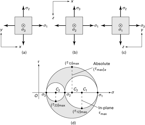
The largest shear stresses occur on planes oriented at 45° to the principal planes. The shear stress is a maximum located as the highest point on the outer circle. The value of the absolute maximum shearing stress is therefore
(1.45)
acting on the planes that bisect the planes of the maximum and minimum principal stresses, as shown in Fig. 1.25b. It is noted that the planes of maximum shear stress may also be ascertained by substituting n2 = 1 – l2 – m2 into Eq. (1.38b), differentiating with respect to l and m, and equating the resulting expressions to zero (Prob. 1.80).
Determining the absolute value of maximum shear stress is significant when designing members made of ductile materials, since the strength of the material depends on its ability to resist shear stress (Sec. 4.6). Obviously, as far as the stress magnitudes are concerned, the largest circle is the most significant one. However, all stresses in their various transformations may play a role in causing failure, and it is usually instructive to plot all three principal circles of stress, as depicted in the figure. An example of this type occurs in thin-walled pressurized cylinders, where σθ = σ1, σa = σ2, and σr = σ3 = 0 at the outer surface (Table 1.1). It is also interesting to note that, in special cases, where two or all principal stresses are equal, a Mohr’s circle becomes a point.
Equations of Three Mohr’s Circles for Stress
It has been demonstrated that, given the values of the principal stresses and of the direction cosines for any oblique plane (Fig. 1.22b), the normal and shear stresses on the plane may be ascertained through the application of Eqs. (1.37) and (1.38). This may also be accomplished by means of a graphical technique due to Mohr [Refs. 1.10 through 1.12]. The latter procedure was used in the early history of stress analysis, but today it is employed only as a heuristic device.
In the following discussion, we demonstrate that the aforementioned equations together with the relation l2 + m2 + n2 = 1 are represented by three circles of stress, and the coordinates (σ, τ) locate a point in the shaded area of Fig. 1.26d [Ref. 1.13]. These simultaneous equations are
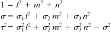
(a)
where l2 ≥ 0, m2 ≥ 0, and n2 ≥ 0. Solving for the direction cosines, results in
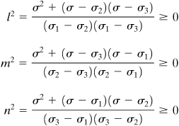
(1.46)
Inasmuch as σ1 > σ2 > σ3, the numerators of Eqs. (1.46) satisfy
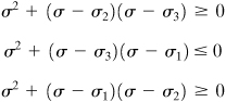
(b)
as the denominators of Eqs. (1.46) are (σ1 – σ2) > 0 and (σ1 – σ3) > 0, (σ2 – σ3) > 0 and (σ2 – σ1) < 0, (σ3 – σ1) < 0 and (σ3 – σ2) < 0, respectively.
Finally, the preceding inequalities may be expressed as follows
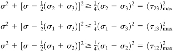
(1.47)
Equations (1.47) represent the formulas of the three Mohr’s circles for stress, shown in Fig. 1.26d. Stress points (σ, τ) satisfying the equations for circles centered at C1 and C2 lie on or outside circles, but for the circle centered at C3 lie on or inside circle. We conclude therefore that an admissible state of stress must lie on Mohr’s circles or within the shaded area enclosed by these circles.
Example 1.8. Analysis of Three-Dimensional Stresses in a Member
The state of stress on an element of a structure is illustrated in Fig. 1.27a. Using Mohr’s circle, determine (a) the principal stresses and (b) the maximum shearing stresses. Show results on a properly oriented element. Also, (c) apply the equations developed in Section 1.14 to calculate the octahedral stresses.
Figure 1.27. Example 1.8. (a) Element in three-dimensional stress; (b) Mohr’s circles of stress; (c) stress element for ![]() .
.
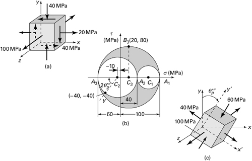
Solution
a. First, Mohr’s circle for the transformation of stress in the xy plane is sketched in the usual manner as shown, centered at C2 with diameter A2A3 (Fig. 1.27b). Next, we complete the three-dimensional Mohr’s circle by drawing two additional circles of diameters A1A2 and A1A3 in the figure. Referring to the circle, the principal stresses are σ1 = 100 MPa, σ2 = 40 MPa, and σ3 = –60 MPa. Angle ![]() , as tan
, as tan ![]() . The results are sketched on a properly oriented element in Fig. 1.27c.
. The results are sketched on a properly oriented element in Fig. 1.27c.
b. The absolute maximum shearing stress, point B3, equals the radius of the circle centered at C3 of diameter A1 A3. Thus,
![]()
The maximum shearing stress occurs on the planes 45° from the y′ and z faces of the element of Fig. 1.27c.
c. The octahedral normal stress, from Eq. (1.44), is
![]()
The octahedral shearing stress, using Eq. (1.43), is
![]()
Comments
A comparison of the results (see Fig. 1.27b) shows that
![]()
That is, the maximum principal stress and absolute maximum shear stress are greater than their octahedral counterparts.
1.16 Boundary Conditions in Terms of Surface Forces
We now consider the relationship between the stress components and the given surface forces acting on the boundary of a body. The equations of equilibrium that must be satisfied within a body are derived in Section 1.8. The distribution of stress in a body must also be such as to accommodate the conditions of equilibrium with respect to externally applied forces. The external forces may thus be regarded as a continuation of the internal stress distribution.
Consider the equilibrium of the forces acting on the tetrahedron shown in Fig. 1.19b, and assume that oblique face ABC is coincident with the surface of the body. The components of the stress resultant p are thus now the surface forces per unit area, or surface tractions, px, py, and pz. The equations of equilibrium for this element, representing boundary conditions, are, from Eqs. (1.26),
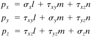
(1.48)
For example, if the boundary is a plane with an x-directed surface normal, Eqs. (1.48) give px = σx, py = τxy, and pz = τxz; under these circumstances, the applied surface force components px, py, and pz are balanced by σx, τxy, and τxz, respectively.
It is of interest to note that, instead of prescribing the distribution of surface forces on the boundary, the boundary conditions of a body may also be given in terms of displacement components. Furthermore, we may be given boundary conditions that prescribe surface forces on one part of the boundary and displacements on another. When displacement boundary conditions are given, the equations of equilibrium express the situation in terms of strain, through the use of Hooke’s law and subsequently in terms of the displacements by means of strain–displacement relations (Sec. 2.3). It is usual in engineering problems, however, to specify the boundary conditions in terms of surface forces, as in Eq. (1.48), rather than surface displacements. This practice is adhered to in this text.
1.17 Indicial Notation
A system of symbols, called indicial notation, index notation, also known as tensor notation, to represent components of force, stress, displacement, and strain is used throughout this text. Note that a particular class of tensor, a vector, requires only a single subscript to describe each of its components. Often the components of a tensor require more than a single subscript for definition. For example, second-order or second-rank tensors, such as those of stress or inertia, require double subscripting: τij, Iij. Quantities such as temperature and mass are scalars, classified as tensors of zero rank.
Tensor or indicial notation, here briefly explored, offers the advantage of succinct representation of lengthy equations through the minimization of symbols. In addition, physical laws expressed in tensor form are independent of the choice of coordinate system, and therefore similarities in seemingly different physical systems are often made more apparent. That is, indicial notation generally provides insight and understanding not readily apparent to the relative newcomer to the field. It results in a saving of space and serves as an aid in nonnumerical computation.
The displacement components u, v, and w, for instance, are written u1, u2, u3 (or ux, uy, uz) and collectively as ui, with the understanding that the subscript i can be 1, 2, and 3 (or x, y, z). Similarly, the coordinates themselves are represented by x1, x2, x3, or simply xi(i = 1, 2, 3), and xx, xy, xz, or xi (i = x, y, z). Many equations of elasticity become unwieldy when written in full, unabbreviated term; see, for example, Eqs. (1.28). As the complexity of the situation described increases, so does that of the formulations, tending to obscure the fundamentals in a mass of symbols. For this reason, the more compact indicial notation is sometimes found in publications.
Two simple conventions enable us to write most equations developed in this text in indicial notation. These conventions, relative to range and summation, are as follows:
Range convention: When a lowercase alphabetic subscript is unrepeated, it takes on all values indicated.
Summation convention: When a lowercase alphabetic subscript is repeated in a term, then summation over the range of that subscript is indicated, making unnecessary the use of the summation symbol.
The introduction of the summation convention is attributable to A. Einstein (1879–1955). This notation, in conjunction with the tensor concept, has far-reaching consequences not restricted to its notational convenience [Refs. 1.14 and 1.15].
References
1.1. TIMOSHENKO, S. P., History of Strength of Materials, Dover, New York, 1983.
1.2. TODHUNTER, L., and PEARSON, K., History of the Theory of Elasticity and the Strength of Materials, Vols. I and II, Dover, New York, 1960.
1.3. LOVE, A. E. H., A Treatise on the Mathematical Theory of Elasticity, 4th ed., Dover, New York, 1944.
1.4. UGURAL, A. C., Stresses in Beams, Plates, and Shells, 3rd ed., CRC Press, Taylor and Francis Group, Boca Raton, Fla., 2010, Sec. 3.2.
1.5. GERE, J., and TIMOSHENKO, S. P., Mechanics of Materials, 3rd ed., PWS-Kent, Boston, 1990.
1.6. UGURAL, A. C., Mechanical Design: An Integrated Approach, McGraw-Hill, New York, 2004, Sec. 1.6.
1.7. UGURAL, A. C., Mechanics of Materials, Wiley, Hoboken, N. J., 2008.
1.8. BORESI, A. P., and CHONG, K. P., Elasticity in Engineering Mechanics, 2nd ed., Wiley, Hoboken, N. J., 2000.
1.9. SOKOLNIKOFF, I. S., Mathematical Theory of Elasticity, 2nd ed., McGraw-Hill, New York, 1956.
1.10. UGURAL, A. C., and FENSTER, S. K., Advanced Strength and Applied Elasticity, 4th ed., Prentice Hall, Englewood Cliffs, N. J., 2003, Sec. 1.15.
1.11. SHAMES, I. H., and COZZARELLI, F. A., Elastic and Inelastic Stress Analysis, Prentice Hall, Englewood Cliffs, N. J., 1992.
1.12. FORD, H., Advanced Mechanics of Materials, 2nd ed., Ellis Horwood, Chichester, England, 1977, Chap. 4.
1.13. HOFFMAN, O., and SACHS, G., Introduction to the Theory of Plasticity for Engineers, McGraw-Hill, New York, 1953.
1.14. REISMANN, H., and PAWLIK, P. S., Elasticity: Theory and Applications, Wiley, Hoboken, N. J., 1980, Chap. 1.
1.15. CHOU, P. C., and PAGANO, N. J., Elasticity, Dover, New York, 1992, Chaps. 8 and 9.
Problems
Sections 1.1 through 1.8
1.1. Two prismatic bars of a by b rectangular cross section are glued as shown in Fig. P1.1. The allowable normal and shearing stresses for the glued joint are 700 and 560 kPa, respectively. Assuming that the strength of the joint controls the design, what is the largest axial load P that may be applied? Use φ = 40°, a = 50 mm, and b = 75 mm.
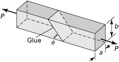
1.2. A prismatic steel bar of a = b = 50-mm square cross section is subjected to an axial tensile load P = 125 kN (Fig. P1.1). Calculate the normal and shearing stresses on all faces of an element oriented at (a) φ = 70°, and (b) φ = 45°.
1.3. A prismatic bar is under an axial load, producing a compressive stress of 75 MPa on a plane at an angle θ = 30° (Fig. P1.3). Determine the normal and shearing stresses on all faces of an element at an angle of θ = 50°.
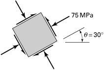
1.4. A square prismatic bar of 1300-mm2 cross-sectional area is composed of two pieces of wood glued together along the x′ plane, which makes an angle θ with the axial direction (Fig. 1.6a). The normal and shearing stresses acting simultaneously on the joint are limited to 20 and 10 MPa, respectively, and on the bar itself, to 56 and 28 MPa, respectively. Determine the maximum allowable axial load that the bar can carry and the corresponding value of the angle θ.
1.5. Calculate the maximum normal and shearing stresses in a circular bar of diameter d = 50 mm subjected to an axial compression load of P = 150 kN through rigid end plates at its ends.
1.6. A frame is formed by two metallic rectangular cross sectional parts soldered along their inclined planes as illustrated in Fig. P1.6. What is the permissible axial load Pall that can be applied to the frame, without exceeding a normal stress of σall or a shearing stress of τall on the inclined plane? Given: a = 10 mm, b = 75 mm, t = 20 mm, θ = 55°, σall = 25 MPa, and τall = 12 MPa. Assumption: Material strength in tension is 90 MPa.
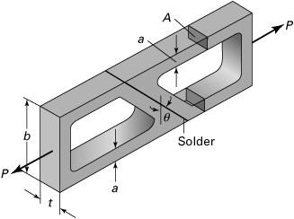
1.7. Redo Prob. 1.6 for the case in which σall = 20 MPa, τall = 8 MPa, and θ = 40°.
1.8. Determine the normal and shearing stresses on an inclined plane at an angle φ through the bar subjected to an axial tensile force of P (Fig. P1.1). Given: a = 15 mm, b = 30 mm, φ = 50°, P = 120 kN.
1.9. Redo Prob. 1.8, for an angle of φ = 30° and P = –100 kN.
1.10. A cylindrical pipe of 160-mm outside diameter and 10-mm thickness, spirally welded at an angle of φ = 40° with the axial (x) direction, is subjected to an axial compressive load of P = 150 kN through the rigid end plates (Fig. P1.10). Determine the normal σx′ and shearing stresses τx′y′ acting simultaneously in the plane of the weld.
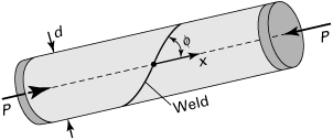
1.11. The following describes the stress distribution in a body (in megapascals):
![]()
Determine the body force distribution required for equilibrium and the magnitude of its resultant at the point x = –10 mm, y = 30 mm, z = 60 mm.
1.12. Given zero body forces, determine whether the following stress distribution can exist for a body in equilibrium:
![]()
Here the c’s are constants.
1.13. Determine whether the following stress fields are possible within an elastic structural member in equilibrium:
a. ![]()
b. ![]()
The c’s are constant, and it is assumed that the body forces are negligible.
1.14. For what body forces will the following stress field describe a state of equilibrium?
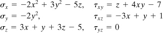
Sections 1.9 through 1.11
1.15. and 1.16. The states of stress at two points in a loaded body are represented in Figs. P1.15 and P1.16. Calculate for each point the normal and shearing stresses acting on the indicated inclined plane. As is done in the derivations given in Section 1.9, use an approach based on the equilibrium equations applied to the wedge-shaped element shown.
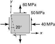
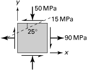
1.17. and 1.18. Resolve Probs. 1.15 and 1.16 using Eqs. (1.18).
1.19. At a point in a loaded machine, the normal and shear stresses have the magnitudes and directions acting on the inclined element shown in Fig. P1.19. What are the stresses σx, σy, and τxy on an element whose sides are parallel to the xy axes?

1.20. The stresses at a point in the enclosure plate of a tank are as depicted in the element of Fig. P1.20. Find the normal and shear stresses at the point on the indicated inclined plane. Show the results on a sketch of properly oriented element.
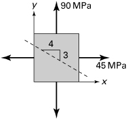
1.21. A welded plate carries the uniform biaxial tension illustrated in Fig. P1.21. Determine the maximum stress σ for two cases: (a) The weld has an allowable shear stress of 30 MPa. (b) The weld has an allowable normal stress of 80 MPa.
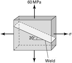
1.22. Using Mohr’s circle, solve Prob. 1.15.
1.23. Using Mohr’s circle, solve Prob. 1.16.
1.24. Using Mohr’s circle, solve Prob. 1.20.
1.25. Using Mohr’s circle, solve Prob. 1.21.
1.26. The states of stress at two points in a loaded beam are represented in Fig. P1.26a and b. Determine the following for each point: (a) The magnitude of the maximum and minimum principal stresses and the maximum shearing stress; use Mohr’s circle. (b) The orientation of the principal and maximum shear planes; use Mohr’s circle. (c) Sketch the results on properly oriented elements. Check the values found in (a) and (b) by applying the appropriate equations.
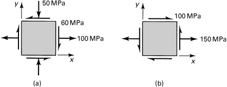
1.27. By means of Mohr’s circle, verify the results given by Eqs. (1.35).
1.28. An element in plane stress (Fig. 1.3b) is subjected to stresses σx = 50 MPa, σy = –190 MPa, and τxy = –70 MPa. Determine the principal stresses and show them on a sketch of a properly oriented element.
1.29. For an element in plane stress (Fig. 1.3b), the normal stresses are σx = 60 MPa and σy = –100 MPa. What is the maximum permissible value of shearing stress τxy if the shearing stress in the material is not to exceed 140 MPa?
1.30. The state of stress on an element oriented at θ = 60° is shown in Fig. P1.30. Calculate the normal and shearing stresses on an element oriented at θ = 0°.
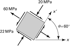
1.31. A thin skewed plate is subjected to a uniform distribution of stress along its sides, as shown in Fig. P1.31. Calculate (a) the stresses σx, σy, σxy, and (b) the principal stresses and their orientations.
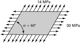
1.32. The stress acting uniformly over the sides of a rectangular block is shown in Fig. P1.32. Calculate the stress components on planes parallel and perpendicular to mn. Show the results on a properly oriented element.
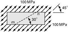
1.33. Redo Prob. 1.31 for the stress distribution shown in Fig. P1.33.
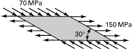
1.34. A thin-walled cylindrical tank of radius r is subjected simultaneously to internal pressure p and a compressive force P through rigid end plates. Determine the magnitude of force P to produce pure shear in the cylindrical wall.
1.35. A thin-walled cylindrical pressure vessel of radius 120 mm and a wall thickness of 5 mm is subjected to an internal pressure of p = 4 MPa. In addition, an axial compression load of P = 30π kN and a torque of T = 10π kN · m are applied to the vessel through the rigid end plates (Fig. P1.35). Determine the maximum shearing stresses and associated normal stresses in the cylindrical wall. Show the results on a properly oriented element.
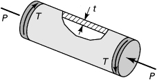
1.36. A pressurized thin-walled cylindrical tank of radius r = 60 mm and wall thickness t = 4 mm is acted on by end torques T = 600 N · m and tensile forces P (Fig. P1.35 with sense of P reversed). The internal pressure is p = 5 MPa. Calculate the maximum permissible value of P if the allowable tensile stress in the cylinder wall is 80 MPa.
1.37. A shaft of diameter d carries an axial compressive load P and two torques T1, T2 (Fig. P1.37). Determine the maximum shear stress at a point A on the surface of the shaft. Given: d = 100 mm, P = 400 kN, T1 = 10 kN · m, and T2 = 2 kN · m.
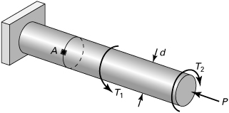
1.38. What are the normal and shearing stresses on the spiral weld of the aluminum shaft of diameter d subjected to an axial load P and a torque T (Fig. P1.38)? Given: P = 120 kN, T = 1.5 kN · m, d = 40 mm, and φ = 50°.
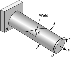
1.39. A hollow generator shaft of 180-mm outer diameter and 120-mm inner diameter carries simultaneously a torque T = 20 kN · m and axial compressive load P = 700 kN. What is the maximum tensile stress?
1.40. A cantilever beam of thickness t is subjected to a constant traction τ0 (force per unit area) at its upper surface, as shown in Fig. P1.40. Determine, in terms of τ0, h, and L, the principal stresses and the maximum shearing stress at the corner points A and B.
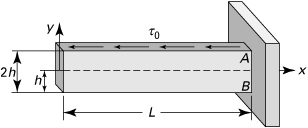
1.41. A hollow shaft of 60-mm outer diameter and 30-mm inner diameter is acted on by an axial tensile load of 50 kN, a torque of 500 N · m and a bending moment of 200 N · m Use Mohr’s circle to determine the principal stresses and their directions.
1.42. Given the stress acting uniformly over the sides of a thin, flat plate (Fig. P1.42), determine (a) the stresses on planes inclined at 20° to the horizontal and (b) the principal stresses and their orientations.
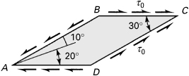
1.43. A steel shaft of radius r = 75 mm is subjected to an axial compression P = 81 kN, a twisting couple T = 15.6 kN · m, and a bending moment M = 13 kN · m at both ends. Calculate the magnitude of the principal stresses, the maximum shear stress, and the planes on which they act in the shaft.
1.44. A structural member is subjected to a set of forces and moments. Each separately produces the stress conditions at a point shown in Fig. P1.44. Determine the principal stresses and their orientations at the point under the effect of combined loading.
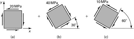
1.45. Redo Prob. 1.44 for the case shown in Fig. P1.45.
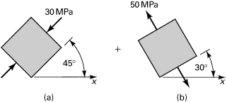
1.46. Redo Prob. 1.44 for the case shown in Fig. P1.46.
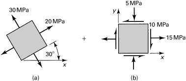
1.47. The shearing stress at a point in a loaded structure is τxy = 40 MPa. Also, it is known that the principal stresses at this point are σ1 = 40 MPa and σ2 = –60 MPa. Determine σx (compression) and σy and indicate the principal and maximum shearing stresses on an appropriate sketch.
1.48. The state of stress at a point in a structure is depicted in Fig. P1.48. Calculate the normal stress σ and the angle θ.
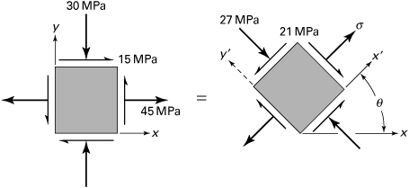
1.49. Acting at a point on a horizontal plane in a loaded machine part are normal stress σy = 20 MPa and a (negative) shearing stress. One principal stress at the point is 10 MPa (tensile), and the maximum shearing stress is of magnitude 50 MPa. Find, by the use of Mohr’s circle, (a) the unknown stresses on the horizontal and vertical planes and (b) the unknown principal stress. Show the principal stresses on a sketch of a properly oriented element.
1.50. For a state of stress at a point in a structure, certain stress components are given for each of the two orientations (Fig. P1.50). Applying transformation equations, calculate stress components σy′ and τx′y′ and the angle θ1 between zero and 90°.
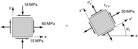
1.51. A solid shaft 200 mm in diameter rotates at f = 20 rps and is subjected to a bending moment of 21π kN · m. Determine the torque T and power P that can also act simultaneously on the shaft without exceeding a resultant shearing stress of 56 MPa and a resultant normal stress of 98 MPa (with f expressed in rps and torque in N · m, P = 2πf · T in watts).
1.52. The cylindrical portion of a compressed-air tank is made of 5-mm-thick plate welded along a helix at an angle of φ = 60° with the axial direction (Fig. P1.52). The radius of the tank is 250 mm. If the allowable shearing stress parallel to the weld is 30 MPa, calculate the largest internal pressure p that may be applied.
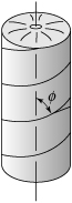
1.53. A thin-walled cylindrical tank is subjected to an internal pressure p and uniform axial tensile load P (Fig. P1.53). The radius and thickness of the tank are r = 0.45 m and t = 5 mm. The normal stresses at a point A on the surface of the tank are restricted to σx′ = 84 MPa and σy′ = 56 MPa, while shearing stress τx′y′ is not specified. Determine the values of p and P. Use θ = 30°.
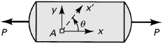
1.54. For a given state of stress at a point in a frame, certain stress components are known for each of the two orientations shown in Fig. P1.54. Using Mohr’s circle, determine the following stress components: (a) τxy and (b) τx′y′ and σy′.
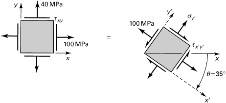
1.55. The state of stress at a point in a machine member is shown in Fig. P1.55. The allowable compression stress at the point is 14 MPa. Determine (a) the tensile stress σx and (b) the maximum principal and maximum shearing stresses in the member. Sketch the results on properly oriented elements.
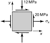
1.56. In Example 1.3, taking σz = 0, investigate the maximum shearing stresses on all possible (three-dimensional) planes.
1.57. A thin-walled pressure vessel of 60-mm radius and 4-mm thickness is made from spirally welded pipe and fitted with two rigid end plates (Fig. P1.57). The vessel is subjected to an internal pressure of p = 2 MPa and a P = 50 kN a axial load. Calculate (a) the normal stress perpendicular to the weld; (b) the shearing stress parallel to the weld.
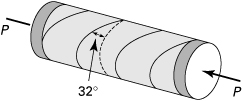
1.58. A thin-walled cylindrical pressure vessel of 0.3-m radius and 6-mm wall thickness has a welded spiral seam at an angle of φ = 30° with the axial direction (Fig. P1.10). The vessel is subjected to an internal gage pressure of p Pa and an axial compressive load of P = 9π kN applied through rigid end plates. Find the allowable value of p if the normal and shearing stresses acting simultaneously in the plane of welding are limited to 21 and 7 MPa, respectively.
Sections 1.12 and 1.13
1.59. The state of stress at a point in an x, y, z coordinate system is
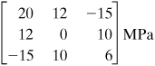
Determine the stresses and stress invariants relative to the x′, y′, z′ coordinate system defined by rotating x, y through an angle of 30° counterclockwise about the z axis.
1.60. Redo Prob. 1.59 for the case in which the state of stress at a point in an x, y, z coordinate system is
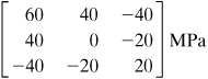
1.61. The state of stress at a point relative to an x, y, z coordinate system is given by
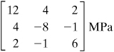
Calculate the maximum shearing stress at the point.
1.62. At a point in a loaded member, the stresses relative to an x, y, z coordinate system are given by
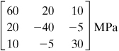
Calculate the magnitude and direction of maximum principal stress.
1.63. For the stresses given in Prob. 1.59, calculate the maximum shearing stress.
1.64. At a specified point in a member, the state of stress with respect to a Cartesian coordinate system is given by
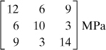
Calculate the magnitude and direction of the maximum principal stress.
1.65. At a point in a loaded structure, the stresses relative to an x, y, z coordinate system are given by
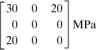
Determine by expanding the characteristic stress determinant: (a) the principal stresses; (b) the direction cosines of the maximum principal stress.
1.66. The stresses (in megapascals) with respect to an x, y, z coordinate system are described by
![]()
At point (3, 1, 5), determine (a) the stress components with respect to x′, y′, z′ if
![]()
and (b) the stress components with respect to x″, y″, z″ if ![]() ,
, ![]() , and n3 = 1. Show that the quantities given by Eq. (1.34) are invariant under the transformations (a) and (b).
, and n3 = 1. Show that the quantities given by Eq. (1.34) are invariant under the transformations (a) and (b).
1.67. Determine the stresses with respect to the x′, y′, z′ axes in the element of Prob. 1.64 if
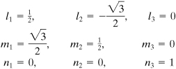
1.68. For the case of plane stress, verify that Eq. (1.33) reduces to Eq. (1.20).
1.69. Obtain the principal stresses and the related direction cosines for the following cases:
a. 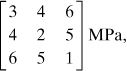
b. 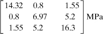
Sections 1.14 through 1.17
1.70. The stress at a point in a machine component relative to an x, y, z coordinate system is given by
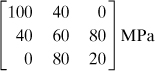
Referring to the parallelepiped shown in Fig. P1.70, calculate the normal stress σ and the shear stress τ at point Q for the surface parallel to the following planes: (a) CEBG, (b) ABEF, (c) AEG. [Hint: The position vectors of points G, E, A and any point on plane AEG are, respectively, rg = 3i, re = 4j, ra = 2k, r = xi + yj + zk. The equation of the plane is given by
(P1.70)
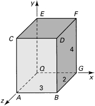
from which
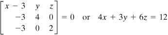
The direction cosines are then
![]()
1.71. Re-solve Prob. 1.70 for the case in which the dimensions of the parallelepiped are as shown in Fig. P1.71.
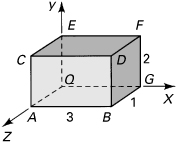
1.72. The state of stress at a point in a member relative to an x, y, z coordinate system is
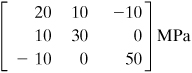
Determine the normal stress σ and the shearing stress τ on the surface intersecting the point and parallel to the plane: 2x + y – 3z = 9.
1.73. For the stresses given in Prob. 1.62, calculate the normal stress σ and the shearing stress τ on a plane whose outward normal is oriented at angles 35°, 60°, and 73.6° with the x, y, and z axes, respectively.
1.74. At a point in a loaded body, the stresses relative to an x, y, z coordinate system are
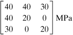
Determine the normal stress σ and the shearing stress τ on a plane whose outward normal is oriented at angles of 40°, 75°, and 54° with the x, y, and z axes, respectively.
1.75. Determine the magnitude and direction of the maximum shearing stress for the cases given in Prob. 1.69.
1.76. The stresses at a point in a loaded machine bracket with respect to the x, y, z axes are given as
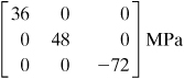
Determine (a) the octahedral stresses; (b) the maximum shearing stresses.
1.77. The state of stress at a point in a member relative to an x, y, z coordinate system is given by
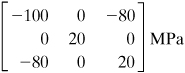
Calculate (a) the principal stresses by expansion of the characteristic stress determinant; (b) the octahedral stresses and the maximum shearing stress.
1.78. Given the principal stresses σ1, σ2, and σ3 at a point in an elastic solid, prove that the maximum shearing stress at the point always exceeds the octahedral shearing stress.
1.79. Determine the value of the octahedral stresses of Prob. 1.64.
1.80. By using Eq. (1.38b), verify that the planes of maximum shearing stress in three dimensions bisect the planes of maximum and minimum principal stresses. Also find the normal stresses associated with the shearing plane by applying Eq. (1.37).
1.81. A point in a structural member is under three-dimensional stress with σx = 100 MPa, σy = 20 MPa, τxy = 60 MPa, and σz, as shown in Fig. P1.81. Calculate (a) the absolute maximum shear stress for σz = 30 MPa; (b) the absolute maximum shear stress for σz = –30 MPa.
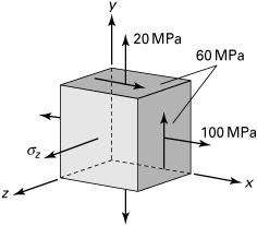
1.82. Consider a point in a loaded body subjected to the stress field represented in Fig. P1.82. Determine, using only Mohr’s circle, the principal stresses and their orientation with respect to the original system.
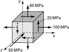
1.83. Re-solve Prob. 1.82 for the case of a point in a loaded body subjected to the following nonzero stress components: σx = 80 MPa, σz = –60 MPa, and τxy = 40 MPa.
1.84. The state of stress at a point in a loaded structure is represented in Fig. P1.84. Determine (a) the principal stresses; (b) the octahedral stresses and maximum shearing stress.
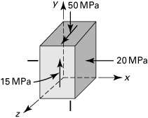
1.85. Find the normal and shearing stresses on an oblique plane defined by ![]() ,
, ![]() and
and ![]() .
.
The principal stresses are σ1 = 35 MPa, σ2 = –14 MPa, and σ3 = –28 MPa. If this plane is on the boundary of a structural member, what should be the values of surface forces px, py, and px on the plane?
1.86. Redo Prob. 1.85 for an octahedral plane, σ1 = 40 MPa, σ2 = 15 MPa, and σ3 = 25 MPa.