Chapter 10. Applications of Energy Methods
10.1 Introduction
As an alternative to the methods based on differential equations as outlined in Section 3.1, the analysis of stress and deformation can be accomplished through the use of energy methods. The latter are predicated on the fact that the equations governing a given stress or strain configuration are derivable from consideration of the minimization of energy associated with deformation, stress, or deformation and stress. Applications of energy methods are effective in situations involving a variety of shapes and variable cross sections and in complex problems involving elastic stability and multielement structures. In particular, strain energy methods offer concise and relatively simple approaches for computation of the displacements of slender structural and machine elements subjected to combined loading.
We shall deal with two principal energy methods.* The first is concerned with the finite deformation experienced by an element under load (Secs. 10.2 to 10.7). The second relies on a hypothetical or virtual variation in stress or deformation and represents one of the variational methods (Secs. 10.8 to 10.11). Energy principles are in widespread use in determining solutions to elasticity problems and obtaining deflections of structures and machines. In this chapter, energy methods are used to determine elastic displacements of statically determinate structures as well as to find the redundant reactions and deflections of statically indeterminate systems. With the exception of Section 10.6, our consideration is limited to linearly elastic material behavior and small displacements.
10.2 Work Done in Deformation
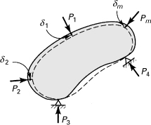
Consider a set of forces (applied forces and reactions) Pk(k ≈ 1, 2,..., m), acting on an elastic body (Fig. 10.1), for example, a beam, truss, or frame. Let the displacement in the direction of Pk of the point at which the force Pk is applied be designated δk. It is clear that δk is attributable to the action of the entire force set, and not to Pk alone. Suppose that all the forces are applied statically, and let the final values of load and displacement be designated Pk and δk. Based on the linear relationship of load and deflection, the work W done by the external force system in deforming the body is given by ![]() .
.
Figure 10.1. Displacements of an elastic body acted on by several forces.
If no energy is dissipated during loading (which is certainly true of a conservative system), we may equate the work done on the body to the strain energy U gained by the body. Thus
(10.1)
While the force set Pk (k = 1, 2, ..., m) includes applied forces and reactions, it is noted that the support displacements are zero, and therefore the support reactions do no work and do not contribute to the preceding summation. Equation (10.1) states simply that the work done by the forces acting on the body manifests itself as elastic strain energy.
To further explore the foregoing concept, consider the body as a combination of small cubic elements. Owing to surface loading, the faces of an element are displaced, and stresses acting on these faces do work equal to the strain energy stored in the element. Consider two adjacent elements within the body. The work done by the stresses acting on two contiguous internal faces is equal but of opposite algebraic sign. We conclude therefore, that the work done on all adjacent faces of the elements will cancel. All that remains is the work done by the stresses acting on the faces that lie on the surface of the body. As the internal stresses balance the external forces at the boundary, the work, whether expressed in terms of external forces (W) or internal stresses (U), is the same.
10.3 Reciprocity Theorem
Consider now two sets of applied forces and reactions: ![]() (k = 1, 2,..., m), set 1;
(k = 1, 2,..., m), set 1; ![]() (j = 1, 2,..., n), set 2. If only the first set is applied, the strain energy is, from Eq. (10.1),
(j = 1, 2,..., n), set 2. If only the first set is applied, the strain energy is, from Eq. (10.1),
(a)
where ![]() are the displacements corresponding to the set
are the displacements corresponding to the set ![]() . Application of only set 2 results in the strain energy
. Application of only set 2 results in the strain energy
(b)
in which ![]() corresponds to the set
corresponds to the set ![]() .
.
Suppose that the first force system ![]() is applied, followed by the second force system
is applied, followed by the second force system ![]() . The total strain energy is
. The total strain energy is
(c)
where U1,2 is the strain energy attributable to the work done by the first force system as a result of deformations associated with the application of the second force system. Because the forces comprising the first set are unaffected by the action of the second set, we may write
(d)
Here ![]() represents the displacements caused by the forces of the second set at the points of application of
represents the displacements caused by the forces of the second set at the points of application of ![]() , the first set. If now the forces are applied in reverse order, we have
, the first set. If now the forces are applied in reverse order, we have
(e)
where
(f)
Here ![]() represents the displacements caused by the forces of set 1 at the points of application of the forces
represents the displacements caused by the forces of set 1 at the points of application of the forces ![]() , set 2.
, set 2.
The loading processes described must, according to the principle of superposition, cause identical stresses within the body. The strain energy must therefore be independent of the order of loading, and it is concluded from Eqs. (c) and (e) that U1,2 = U2,1. We thus have
(10.2)
Expression (10.2) is the reciprocity or reciprocal theorem credited to E. Betti and Lord Rayleigh: The work done by one set of forces owing to displacements due to a second set is equal to the work done by the second system of forces owing to displacements due to the first.
The utility of the reciprocal theorem lies principally in its application to the derivation of various approaches rather than as a method in itself.
10.4 Castigliano’s Theorem
First formulated in 1879, Castigliano’s theorem is in widespread use because of the ease with which it is applied to a variety of problems involving the deformation of structural elements, especially those classed as statically indeterminate. There are two theorems credited to Castigliano. In this section we discuss the one restricted to structures composed of linearly elastic materials, that is, those obeying Hooke’s law. For these materials, the strain energy is equal to the complementary energy: U = U*. In Section 10.9, another form of Castigliano’s theorem is introduced that is appropriate to structures that behave nonlinearly as well as linearly. Both theorems are valid for the cases where any change in structure geometry owing to loading is so small that the action of the loads is not affected.
Refer again to Fig. 10.1, which shows an elastic body subjected to applied forces and reactions, Pk(k = 1, 2, ..., m). This set of forces will be designated set 1. Now let one force of set 1, Pi, experience an infinitesimal increment ΔPi. We designate as set 2 the increment ΔPi. According to the reciprocity theorem, Eq. (10.2), we may write
(a)
where Δδk is the displacement in the direction and, at the point of application, of Pk attributable to the forces of set 2, and δi is the displacement in the direction and, at the point of application, of Pi due to the forces of set 1.
The incremental strain energy ΔU = ΔU2 + ΔU1,2 associated with the application of ΔPi is, from Eqs. (b) and (d) of Section 10.3, ![]() . Substituting Eq. (a) into this, we have
. Substituting Eq. (a) into this, we have ![]() . Now divide this expression by ΔPi and take the limit as the force ΔPi approaches zero. In the limit, the displacement Δδi produced by ΔPi vanishes, leaving
. Now divide this expression by ΔPi and take the limit as the force ΔPi approaches zero. In the limit, the displacement Δδi produced by ΔPi vanishes, leaving
(10.3)
This is known as Castigliano’s second theorem: For a linear structure, the partial derivative of the strain energy with respect to an applied force is equal to the component of displacement at the point of application of the force that is in the direction of the force.
It can similarly be demonstrated that
(10.4)
where Ci and θi are, respectively, the couple (bending or twisting) moment and the associated rotation (slope or angle of twist) at a point.
In applying Castigliano’s theorem, the strain energy must be expressed as a function of the load. For example, the expression for the strain energy in a straight or curved slender bar (Sec. 5.13) subjected to a number of common loads (axial force N, bending moment M, shearing force V, and torque T) is, from Eqs. (2.59), (2.63), (5.64), and (2.62),
(10.5)
in which the integrations are carried out over the length of the bar. Recall that the term given by the last integral is valid only for a circular cross-sectional area. The displacement at any point in the bar may then readily be found by applying Castigliano’s theorem. Inasmuch as the force P is not a function of x, we can perform the differentiation of U with respect to P under the integral. In so doing, the displacement is obtained in the following convenient form:
(10.6)
Similarly, an expression may be written for the angle of rotation:
(10.7)
For a slender beam, as observed in Section 5.4, the contribution of the shear force V to the displacement is negligible.
Referring to Section 2.13, in the case of a plane truss consisting of n members of length Lj, axial rigidity AjEj, and internal axial force Nj, the strain energy can be found from Eq. (2.59) as follows:
(10.8)
The displacement δi of the point of application of load P is therefore
(10.9)
Here the axial force Nj in each member may readily be determined using the method of joints or method of sections. The former consists of analyzing the truss joint by joint to find the forces in members by applying the equations of equilibrium at each joint. The latter is often employed for problems where the forces in only a few members are to be obtained.
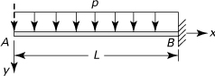
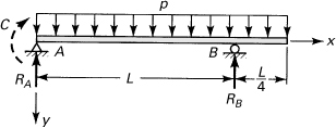
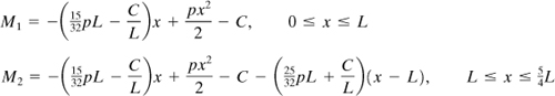
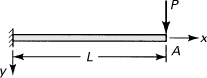
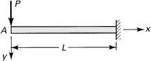
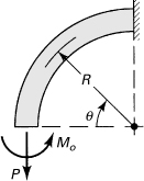
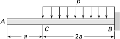
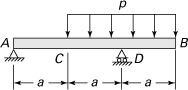
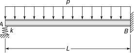
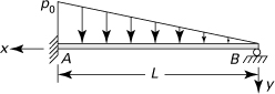
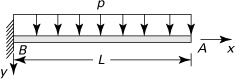
A final point to be noted that, when it is necessary to determine the deflection at a point at which no load acts, the problem is treated as follows. A fictitious load Q (or C) is introduced at the point in question in the direction of the desired displacement δ (or θ). The displacement is then found by applying Castigliano’s theorem, setting Q = 0 (or C = 0) in the final result. Consider, for example, the cantilever beam AB supporting a uniformly distributed load of intensity p (Fig. 10.2). To determine the deflection at A, we apply a fictitious load Q, as shown by the dashed line in the figure. Expressions for the moment and its derivative with respect to Q are, respectively,
![]()
Substituting these into Eq. (10.6) and making Q = 0 results in
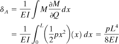
Since the fictitious load was directed downward, the positive sign means that the deflection δA is also downward.
Figure 10.2. A cantilever beam with a uniform load.
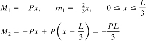
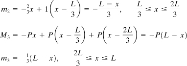
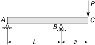
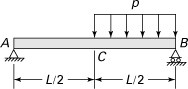
Example 10.1. Slope of a Beam with an Overhang
Determine the slope of the elastic curve at the left support of the uniformly loaded beam shown in Fig. 10.3.
Figure 10.3. Example 10.1. Uniformly loaded beam with an overhang.
Solution
As a slope is sought, a fictitious couple moment C is introduced at point A. Applying the equations of statics, the reactions are found to be
![]()
The following expressions for the moments are thus available:
The slope at A is now found from Eq. (10.7):
![]()
Setting C = 0 and integrating, we obtain θA = 7pL3/192 EI.
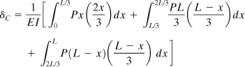
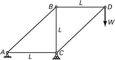
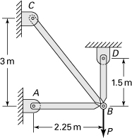
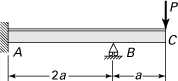
Example 10.2. Deflection of a Pin-Connected Structure
A load P is applied at B to two bars of equal length L but different cross-sectional areas and modulii of elasticity (Fig. 10.4a). Determine the horizontal displacement δB of point B.
Figure 10.4. Example 10.2. Two-bar structure carries a load P.
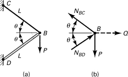
Solution
A fictitious load Q is applied at B. The forces in the bars are determined by considering the equilibrium of the free-body diagram of pin B (Fig. 10.4b):
(NBC + NBD)sinθ = P
(NBC – NBD)cosθ = Q
or
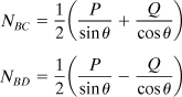
(b)
Differentiating these expressions with respect to Q,
![]()
Applying Castigliano’s theorem, Eq. (10.6),
![]()
Introducing Eqs. (b) and setting Q = 0 yields the horizontal displacement of the pin under the given load P:
(c)
A check is provided in that, in the case of two identical rods, the preceding expression gives δB = 0, a predictable result.
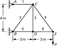
Example 10.3. Three-Bar Truss
The simple pin-connected truss shown in Fig. 10.5 supports a force P. If all members are of equal rigidity AE, what is the deflection of point D?
Figure 10.5. Example 10.3. A truss supports a load P.
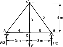
Solution
Applying the method of joints at points A and C and taking symmetry into account, we obtain N1 = N2 = 5P/8, N4 = N5 = 3P/8, and N3 = P. Castigliano’s theorem, Eq. (10.9), may be written
(d)
where n = 5. Substituting the values of axial forces in terms of applied load into Eq. (d) leads to
![]()
from which δD = 35p/4AE.
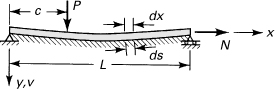
Example 10.4. Thick-Walled Half Ring
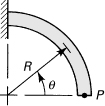
A load P of 5 kN is applied to a steel curved bar as depicted in Fig. 10.6a. Determine the vertical deflection of the free end by considering the effects of the internal normal and shear forces in addition to the bending moment. Let E = 200 GPa and G = 80 GPa.
Figure 10.6. Example 10.4. (a) A thick-walled curved bar is fixed at one end and supports a load P at its free end; (b) segment of the bar.
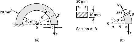
Solution
A free-body diagram of a portion of the bar subtended by angle θ is shown in Fig. 10.6b, where the internal forces (N and V) and moment (M) are positive as indicated. Referring to the figure,
(10.10)
Thus,
![]()
The form factor for shear for the rectangular section is ![]() (Table 5.1). Substituting the preceding expressions into Eq. (10.6) with dx = R dθ, we have
(Table 5.1). Substituting the preceding expressions into Eq. (10.6) with dx = R dθ, we have
![]()
Integration of the foregoing results in
(10.11)
Geometric properties of the section of the bar are
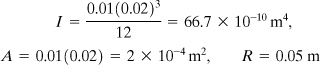
Insertion of the data into Eq. (10.11) gives
δv = (2.21 + 0.03 + 0.01) × 10–3 = 2.25 mm
Comment
Note that if the effects of the normal and shear forces are omitted
δv = 2.21 mm
with a resultant error in deflection of approximately 1.8%. For this curved bar, in which R/c = 5, the contribution of V and N to the displacement can thus be neglected. It is common practice to omit the first and the third terms in Eqs. (10.6) and (10.7) when R/c > 4 (Sec. 5.13).
Example 10.5. Analysis of a Piping System
A piping system expansion loop is fabricated of pipe of constant size and subjected to a temperature differential ΔT (Fig. 10.7). The overall length of the loop and the coefficient of thermal expansion of the tubing material are L and α, respectively.
Figure 10.7. Example 10.5. Expansion loop is subjected to a temperature change.
Determine, for each end of the loop, the restraining bending moment M and force N induced by the temperature change.
Solution
In labeling the end points for each segment, the symmetry about a vertical axis through point A is taken into account, as shown in the figure. Expressions for the moments, associated with segments DC, CB, and BA, are, respectively,
(e)
Upon application of Eqs. (10.3) and (10.4), the end deflection and end slope are found to be
(f)
(g)
Substitution of Eqs. (e) into Eq. (f) results in
(h)
Similarly, Eqs. (g) and (e) lead to
(10.12a)
The deflections at G owing to the temperature variation and end restraints must be equal; that is,
(10.12b)
Expressions (h) and (10.12) are then solved to yield the unknown reactions N and M in terms of the given properties and loop dimensions.
10.5 Unit- or Dummy-Load Method
Recall that the deformation at a point in an elastic body subjected to external loading Pi, expressed in terms of the moment produced by the force system, is, according to Castigliano’s theorem,
(a)
For small deformations of linearly elastic materials, the moment is linearly proportional to the external loads, and consequently we are justified in writing M = mPi, with m independent of Pi. It follows that ∂M/∂Pi = m, the change in the bending moment per unit change in Pi, that is, the moment caused by a unit load.
The foregoing considerations lead to the unit-load or dummy-load approach, which finds extensive application in structural analysis. From Eq. (a),
(10.13)
In a similar manner, the following expression is obtained for the change of slope:
(10.14)
Here m′ = ∂M/∂Ci represents the change in the bending moment per unit change in Ci, that is, the change in bending moment caused by a unit-couple moment.
Analogous derivations can be made for the effects of axial, shear, and torsional deformations by replacing m in Eq. (10.13) with n = ∂N/∂Pi, v = ∂V/∂Pi, and t = ∂T/∂Pi, respectively. It can also readily be demonstrated that, in the case of truss, Eq. (10.9) has the form
(10.15)
wherein AE is the axial rigidity. The quantity nj = ∂Nj/∂Pi represents the change in the axial forces Nj owing to a unit value of load Pi.
Example 10.6. Deflection of a Simple Beam with Two Loads
Derive an expression for the deflection of point C of the simply supported beam shown in Fig. 10.8a.
Figure 10.8. Example 10.6. (a) Actual loading; (b) unit loading.
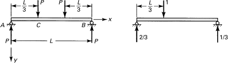
Solution
Figure 10.8b shows the dummy load of 1 N and the reactions it produces. Note that the unit load is applied at C because it is the deflection of C that is required. Referring to the figure, the following moment distributions are obtained:
Here the M’s refer to Fig. 10.8a and the m’s to Fig. 10.8b. The vertical deflection at C is then, from Eq. (10.14),
The solution, after integration, is found to be δC = 5PL3/162EI.
10.6 Crotti–Engesser Theorem
Consider a set of forces acting on a structure that behaves nonlinearly. Let the displacement of the point at which the force Pi is applied, in the direction of Pi, be designated δi. This displacement is to be determined. The problem is the same as that stated in Section 10.4, but now it will be expressed in terms of Pi and the complementary energy U* of the structure, the latter being given by Eq. (2.49).
In deriving the theorem, a procedure is employed similar to that given in Section 10.4. Thus, U is replaced by U* in Castigliano’s second theorem, Eq. (10.3), to obtain
(10.16)
This equation is known as the Crotti–Engesser theorem: The partial derivative of the complementary energy with respect to an applied force is equal to the component of the displacement at the point of application of the force that is in the direction of the force. Obviously, here the complementary energy must be expressed in terms of the loads.
Example 10.7. Nonlinearly Elastic Structure
A simple truss, constructed of pin-connected members 1 and 2, is subjected to a vertical force P at joint B (Fig. 10.9a). The bars are made of a nonlinearly elastic material displaying the stress–strain relation σ = Kε1/2 equally in tension and compression (Fig. 10.9b). Here the strength coefficient K is a constant. The cross-sectional area of each member is A. Determine the vertical deflection of joint B.
Figure 10.9. Example 10.7. Two-bar structure with material nonlinearity.
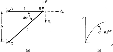
Solution
The volume of member 1 is Ab and that of member 2 is ![]() . The total complementary energy of the structure is therefore
. The total complementary energy of the structure is therefore
(a)
The complementary energy densities are, from Eq. (2.49),
(b)
where σ1 and σ2 are the stresses in bars 1 and 2. Upon introduction of Eqs. (b) into (a), we have
(c)
From static equilibrium, the axial forces in 1 and 2 are found to be P and ![]() , respectively. Thus, σ1 = P/A (tension) and
, respectively. Thus, σ1 = P/A (tension) and ![]() (compression), which when introduced into Eq. (c) yields
(compression), which when introduced into Eq. (c) yields
(d)
Applying Eq. (10.16), the vertical deflection of B is found to be
![]()
Another approach to the solution of this problem is given in Example 10.11.
10.7 Statically Indeterminate Systems
To supplement the discussion of statically indeterminate systems given in Section 5.11, energy methods are now applied to obtain the unknown, redundant forces (moments) in such systems. Consider, for example, the beam system of Fig. 10.3 rendered statically indeterminate by the addition of an extra or redundant support at the right end (not shown in the figure). The strain energy is, as before, written as a function of all external forces, including both applied loads and reactions. Castigliano’s theorem may then be applied to derive an expression for the deflection at point B, which is clearly zero:
(a)
Expression (a) and the two equations of statics available for this force system provide the three equations required for the determination of the three unknown reactions.
Extending this reasoning to the case of a statically indeterminate beam with n redundant reactions, we write
(b)
The equations of statics together with the equations of the type given by Eq. (b) constitute a set sufficient for solution of all the reactions. This basic concept is fundamental to the analysis of structures of considerable complexity.
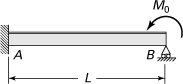
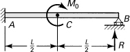
Example 10.8. Spring-Propped Cantilever Beam
The built-in beam shown in Fig. 10.10 is supported at one end by a spring of constant k. Determine the redundant reaction.
Figure 10.10. Example 10.8. A propped cantilever beam with load P.
Solution
The expressions for the moments are
Applying Castigliano’s theorem to obtain the deflection at point D, δD = ∂U/∂RD, we have
![]()
from which ![]() . Equilibrium of vertical forces yields
. Equilibrium of vertical forces yields
(10.17)
Note that were the right end rigidly supported, δD would be equated to zero.
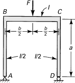
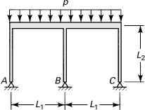
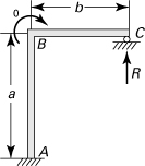
Example 10.9. Rectangular Frame
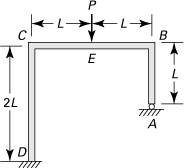
A rectangular frame of constant EI is loaded as shown in Fig. 10.11a. Assuming the strain energy to be attributable to bending alone, determine the increase in distance between the points of application of the load.
Figure 10.11. Example 10.9. (a) A frame; (b) free-body diagram of part AB.
Solution
The situation described is statically indeterminate. For reasons of symmetry, we need analyze only one quadrant. Because the slope B is zero before and after application of the load, the segment may be treated as fixed at B (Fig. 10.11b). The moment distributions are
![]()
Since the slope is zero at A, we have
![]()
from which MA = Pb2/4(a + b). By applying Castigliano’s theorem, the relative displacement between the points of application of load is then found to be δ = Pb3(4a + b)/12EI(a + b).
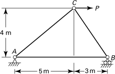
Example 10.10. Member Forces in a Three-Bar Truss
A symmetric plane structure constructed of three bars of equal axial rigidity AE is subjected to a load P at joint D, as illustrated in Fig. 10.12a. Using Castigliano’s theorem, find the force in each bar.
Figure 10.12. Example 10.10. (a) A plane structure; (b) free-body diagram of joint D.
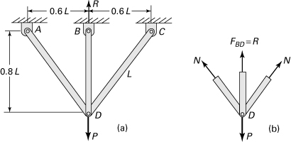
Solution
The structure is statically indeterminate to the first degree. The reaction R at B, which is equal to the force in the bar BD, is selected as redundant. Due to symmetry, the forces AD and CD are each equal to N. The condition of equilibrium of forces at joint D (Fig. 10.12b), gives
(c)
Substituting the foregoing relation and the given numerical values into Eq. (10.34), we find the deflection at joint B in the form
(d)
Since the support B does not move, we set δB = 0 in Eq. (d). In so doing, the reaction at B is determined as follows R = 0.494P. The forces in the members, from Eq. (c), are thus
![]()
and
NBD = R = 0.494P
10.8 Principle of Virtual Work
In this section a second type of energy approach is explored, based on a hypothetical variation of deformation. This method, as is demonstrated, lends itself to the expeditious solution of a variety of important problems.
Consider a body in equilibrium under a system of forces. Accompanying a small displacement within the body, we expect a change in the original force system. Suppose now that an arbitrary incremental displacement occurs, termed a virtual displacement. This displacement need not actually take place and need not be infinitesimal. If we assume the displacement to be infinitesimal, as is usually done, it is reasonable to regard the system of forces as unchanged. In connection with virtual work, we shall use the symbol δ to denote a virtual infinitesimally small quantity.
Recall from particle mechanics that for a point mass, unconstrained and thereby free to experience arbitrary virtual displacements δu, δv, and δw, the virtual work accompanying these displacements is ΣFx δu, ΣFyδv, and ΣFz δw, where ΣFx, ΣFy, and ΣFz are the force resultants. If the particle is in equilibrium, it follows that the virtual work must vanish, since ΣFx = ΣFy = ΣFz = 0. This is the principle of virtual work.
For an elastic body, it is necessary to impose a number of restrictions on the arbitrary virtual displacements. To begin with, these displacements must be continuous and their derivatives must exist. In this way, material continuity is assured. Because certain displacements on the boundary may be dictated by the circumstances of a given situation (boundary conditions), the virtual displacements at such points on the boundary must be zero. A virtual displacement results in no alteration in the magnitude or direction of external and internal forces. The imposition of a virtual displacement field on an elastic body does, however, result in the imposition of an increment in the strain field.
To determine the virtual strains, replace the displacements u, v, and w by virtual displacements δu, δv, and δw in the definition of the actual strains, Eq. (2.4):
![]()
The strain energy δU acquired by a body of volume V as a result of virtual straining is, by application of Eq. (2.47) together with the second of Eqs. (2.44),
(10.18)
Note the absence in this equation of any term involving a variation in stress. This is attributable to the assumption that the stress remains constant during application of virtual displacement.
The variation in strain energy may be viewed as the work done against the mutual actions between the infinitesimal elements composing the body, owing to the virtual displacements (Sec. 10.2). The virtual work done in an elastic body by these mutual actions is therefore –δU.
Consider next the virtual work done by external forces. Again suppose that the body experiences virtual displacements δu, δv, and δw. The virtual work done by a body force F per unit volume and a surface force p per unit area is
(10.19)
where A is the boundary surface. We have already stated that the total work done during the virtual displacement is zero: δW – δU = 0. The principle of virtual work for an elastic body is therefore expressed as follows:
(10.20)
10.9 Principle of Minimum Potential Energy
As the virtual displacements result in no geometric alteration of the body and as the external forces are regarded as constants, Eq. (10.20) may be rewritten
(10.21a)
or, briefly,
(10.21b)
Here it is noted that δ has been removed from under the integral sign. The term Π = U – W is called the potential energy, and Eq. (10.21) represents a condition of stationary potential energy of the system.
It can be demonstrated that, for stable equilibrium, the potential energy is a minimum. Only for displacements that satisfy the boundary conditions and the equilibrium conditions will Π assume a minimum value. This is called the principle of minimum potential energy.
Consider now the case in which the loading system consists only of forces applied at points on the surface of the body, denoting each point force by Pi and the displacement in the direction of this force by δi (corresponding to the equilibrium state). From Eq. (10.21), we have
![]()
The principle of minimum potential energy thus leads to
(10.22)
The preceding means that the partial derivative of the stain energy with respect to a displacement δi equals the force acting in the direction of δi at the point of application of Pi. Equation (10.22) is known as Castigliano’s first theorem. This theorem, as with the Crotti–Engesser theorem, may be applied to any structure, linear or nonlinear.
Example 10.11. Nonlinearly Elastic Basic Truss
Determine the vertical displacement δv and the horizontal displacement δh of the joint B of the truss described in Example 10.7.
Solution
First introduce the unknown vertical and horizontal displacements at the joint shown by dashed lines in Fig. 10.9a. Under the influence of δv, member 1 does not deform, while member 2 is contracted by δv/2b per unit length. Under the influence of δh, member 1 elongates by δh/b, and member 2 by δh/2b per unit length. The strains produced in members 1 and 2 under the effect of both displacements are then calculated from
(a)
where ε1 is an elongation and ε2 is a shortening. Members 1 and 2 have volumes Ab and ![]() , respectively. Next, the total strain energy of the truss, from Eq. (a) of Section 2.13, is determined as follows:
, respectively. Next, the total strain energy of the truss, from Eq. (a) of Section 2.13, is determined as follows:
![]()
Upon substituting σ = Kε1/2 and Eqs. (a), and integrating, this becomes
![]()
Now we apply Castigliano’s theorem in the horizontal and vertical directions at B, respectively:
Simplifying and solving these expressions simultaneously, the joint displacements are found to be
(b)
The stress–strain law, together with Eqs. (a) and (b), yields the stresses in the members if required:
![]()
The axial forces are therefore
![]()
Here N1 is tensile and N2 is compressive. It is noted that, for the statically determinate problem under consideration, the axial forces could readily be determined from static equilibrium. The solution procedure given here applies similarly to statically indeterminate structures as well as to linearly elastic structures.
10.10 Deflections by Trigonometric Series
Certain problems in the analysis of structural deformation, mechanical vibration, heat transfer, and the like, are amenable to solution by means of trigonometric series. This approach offers an important advantage: a single expression may apply to the entire length of the member. The method is now illustrated using the case of a simply supported beam subjected to a moment at point A (Fig. 10.13a). The solution by trigonometric series can also be employed in the analysis of beams having any other type of end condition and beams under combined loading [Refs. 10.5 and 10.9], as demonstrated in Examples 10.12 and 10.13.
Figure 10.13. (a) Simple beam subjected to a moment Mo at an arbitrary distance c from the left support; (b) and (c) deflection curve represented by the first and second terms of a Fourier series, respectively.
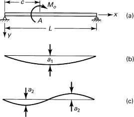
The deflection curve can be represented by a Fourier sine series:
(10.23)
The end conditions of the beam (v = 0, v″ = 0 at x = 0, x = L) are observed to be satisfied by each term of this infinite series. The first and second terms of the series are represented by the curves in Fig. 10.13b and c, respectively. As a physical interpretation of Eq. (10.23), consider the true deflection curve of the beam to be the superposition of sinusoidal curves of n different configurations. The coefficients an of the series are the maximum coordinates of the sine curves, and the n’s indicate the number of half-waves in the sine curves. It is demonstrable that, when the coefficients an are determined properly, the series given by Eq. (10.23) can be used to represent any deflection curve [Ref. 10.10]. By increasing the number of terms in the series, the accuracy can be improved.
To evaluate the coefficients, the principle of virtual work will be applied. The strain energy of the system, from Eqs. (5.62) and (10.23), is written
(a)
Expanding the term in brackets,
![]()
Since for the orthogonal functions sin(mπx/L) and sin(nπx/L) it can be shown by direct integration that
(10.24)
Eq. (a) gives then
(10.25)
The virtual work done by a moment Mo acting through a virtual rotation at A increases the strain energy of the beam by δU:
(b)
Therefore, from Eqs. (10.25) and (b), we have
![]()
which leads to
![]()
Upon substitution of this for an in the series given by Eq. (10.23), the equation for the deflection curve is obtained in the form
(10.26)
Through the use of this infinite series, the deflection for any given value of x can be calculated.
Example 10.12. Cantilever Beam under an End Load
Derive an expression for the deflection of a cantilever beam of length L subjected to a concentrated force P at its free end (Fig. 10.14).
Figure 10.14. Example 10.12. Cantilever beam with a load P at its end.
Solution
The origin of the coordinates is located at the fixed end. Let us represent the deflection by the infinite series
(10.27)
It is clear that Eq. (10.27) satisfies the conditions related to the slope and deflection at x = 0: v = 0, dv/dx = 0. The strain energy of the system is
![]()
Squaring the bracketed term and noting that the orthogonality relationship yields
(10.28)
we obtain
(c)
Application of the principle of virtual work gives P δvE = δU. Thus,
![]()
from which an = 32PL3/n4π4EI. The beam deflection is obtained by substituting the value of an obtained into Eq. (10.27). At x = L, disregarding terms beyond the first three, we obtain vmax = PL3/3.001EI. The exact solution due to bending is PL3/3EI (Sec. 5.4).
Example 10.13. Beam on Elastic Foundation with a Concentrated Load
Determine the equation of the deflection curve of a beam supported at its ends and lying on an elastic foundation of modulus k, subjected to concentrated load P and axial tensile load N (Fig. 10.15).
Figure 10.15. Example 10.13. A simply supported beam resting on an elastic foundation.
Solution
Assume, as the deflection curve, a Fourier sine series, given by Eq. (10.23), which satisfies the end conditions. Denote the arc length of beam segment by ds (Fig. 10.15). To determine the work done by this load, we require the displacement du = ds – dx experienced by the beam in the direction of axial load N:
![]()
Noting that for (dv/dx)2 ≪ 1,
![]()
we obtain
(10.29)
The total energy will be composed of four principal sources: beam bending, tension, transverse loading, and foundation displacement. Strain energy in bending in the beam, from Eq. (10.25), is
(c)
Strain energy owing to the deformation of the elastic foundation is determined as follows:
(10.30)
Work done against the axial load due to shortening u of the span, using Eq. (10.29), is
(10.31)
(10.32)
Application of the principle of virtual work, Eq. (10.20), leads to the following expression:
![]()
After determining an from the preceding and substituting in the series Eq. (10.23), we obtain the deflection curve of the beam:
(10.33)
When the axial load is compressive, contrary to this example, we need to reverse the sign of N in Eq. (10.33). Clearly, the same relationship applies if there is no axial load present (N = 0) or when the foundation is absent (k = 0) and the beam is merely supported at its ends.
Consider, for instance, the case in which load P is applied at the center of the span of a simply supported beam. To calculate the deflection under the load, the values x = c = L/2, N = 0, and k = 0 are substituted into Eq. (10.33):
![]()
The series is rapidly converging, and the first few terms provide the deflection to a high degree of accuracy. Using only the first term of the series, we have
![]()
Comment
Comparing this with the exact solution, we obtain 48.7 instead of 48 in the denominator of the expression. The error in using only the first term of the series is thus approximately 1.5%; the accuracy is sufficient for many practical purposes.
10.11 Rayleigh–Ritz Method
The Rayleigh–Ritz method offers a convenient procedure for obtaining solutions by the principle of minimum potential energy. This method was originated by Lord Rayleigh, and a generalization was contributed by W. Ritz. In this section, application of the method to the determination of the beam displacements is discussed. In Chapters 11 and 13, respectively, the procedure will also be applied to problems involving buckling of columns and bending of plates.
The essentials of the Rayleigh–Ritz method may be described as follows. First assume an expression for the deflection curve, also called the displacement function of the beam, in the form of a series containing unknown parameters an(n = 1, 2, ...). This series function is such that it satisfies the geometric boundary conditions. These describe any end constraints pertaining to deflections and slopes. Another kind of condition, a static boundary condition, which equates the internal forces (and moments) at the edges of the member to prescribed external forces (and moments), need not be fulfilled. Next, using the assumed solution, determine the potential energy Π in terms of an. This indicates that the an’s govern the variation of the potential energy. As the potential energy must be a minimum at equilibrium, the Rayleigh–Ritz method is stated as follows:
(10.34)
This condition represents a set of algebraic equations that are solved to yield the parameters an. Substituting these values into the assumed function, we obtain the solution for a given problem. In general, only a finite number of parameters can be employed, and the solution found is thus only approximate. The accuracy of approximation depends on how closely the assumed deflection shape matches the exact shape. With some experience, the analyst will be able to select a satisfactory displacement function.
The method is illustrated in the solution of the following sample problem.
Example 10.14. Analysis of a Simple Beam under Uniform Load
A simply supported beam of length L is subjected to uniform loading p per unit length. Determine the deflection v(x) by employing (a) a power series and (b) a Fourier series.
Solution
Let the origin of the coordinates be placed at the left support (Fig. 10.16).
Figure 10.16. Example 10.14. A simple beam carries a load of intensity p.
a. Assume a solution of polynomial form:
(a)
Note that this choice enables the deflection to vanish at either boundary. Consider now only the first term of the series:
(b)
The corresponding potential energy, Π= U – W, is
![]()
From the minimizing condition, Eq. (10.34), we obtain a1 = pL2/24EI. The approximate displacement is therefore
![]()
which at midspan becomes vmax = pL4/96EI. This result may be compared with the exact solution due to bending, vmax = pL4/76.8EI, indicating an error in maximum deflection of roughly 17%. An improved approximation is obtained when two terms of the series given by Eq. (a) are retained. The same procedure now yields a1 = pL2/24EI and a2 = p/24EI, so that
(10.35)
At midspan, expression (10.35) provides the exact solution. The foregoing is laborious and not considered practical when compared with the approach given next.
b. Now suppose a solution of the form
(c)
The boundary conditions are satisfied inasmuch as v and v″ both vanish at either end of the beam. We now substitute v and its derivatives into Π = U – W. Employing Eq. (10.24), we obtain, after integration,
![]()
Observe that if n is even, the second term vanishes. Thus,
![]()
and Eq. (10.34) yields an = 4pL4/EI(nπ)5, n = 1, 3, 5, .... The deflection at midspan is, from Eq. (c),
(10.36)
Dropping all but the first term, vmax = pL4/76.5EI. The exact solution is obtained when all terms in the series (c) are retained. Evaluation of all terms in the series may not always be possible, however.
Comment
It should be noted that the results obtained in this example, based on only one or two terms of the series, are remarkably accurate. So few terms will not, in general, result in such accuracy when applying the Rayleigh–Ritz method.
References
10.1. LANGHAAR, H. L., Energy Methods in Applied Mechanics, Krieger, Melbourne, Fla., 1989.
10.2. SOKOLNIKOFF, I. S., Mathematical Theory of Elasticity, 2nd ed., Krieger, Melbourne, Fla., 1986, Chap. 7.
10.3. ODEN, J. T., and RIPPERGER, E. A., Mechanics of Elastic Structures, 2nd ed., McGraw-Hill, New York, 1951.
10.4. UGURAL, A. C., Stresses in Beams, Plates, and Shells, 3rd ed., CRC Press, Taylor and Francis Group, Boca Raton, Fla., 2010.
10.5. FLUGGE, W., ed., Handbook of Engineering Mechanics, McGraw-Hill, New York, 1968, Sec. 31.5.
10.6. FAUPPEL, J. H., and FISHER, F. E., Engineering Design, 2nd ed., Wiley, Hoboken, N.J., 1986.
10.7. UGURAL, A. C., Mechanics of Materials, Wiley, Hoboken, N.J., 2008.
10.8. BURR, A. H., and CHEATHAM, J. B., Mechanical Design, 2nd ed., Prentice Hall, Upper Saddle River, N.J., 1995.
10.9. TIMOSHENKO, S. P., and GERE, J. M., Theory of Elastic Stability, 3rd ed., McGraw-Hill, New York, 1970, Sec. 1.11.
10.10. SOKOLNIKOFF, I. S., and REDHEFFER, R. M., Mathematics of Physics and Modern Engineering, 2nd ed., McGraw-Hill, New York, 1966, Chap. l.
Problems
Sections 10.1 through 10.7
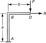
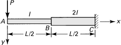
10.1. A cantilever beam of constant AE and EI is loaded as shown in Fig. P10.1. Determine the vertical and horizontal deflections and the angular rotation of the free end, considering the effects of normal force and bending moment. Employ Castigliano’s theorem.
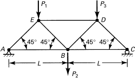
10.2. The truss shown in Fig. P10.2 supports concentrated forces of P1 = P2 = P3 = 45 kN. Assuming all members are of the same cross section and material, find the vertical deflection of point B in terms of AE. Take L = 3 m. Use Castigliano’s theorem.
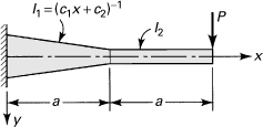
10.3. The moments of inertia of the tapered and constant area segments of the cantilever beam shown in Fig. P10.3 are given by I1 = (c1x + c2)–1 and I2, respectively. Determine the deflection of the beam under a load P. Use Castigliano’s theorem.
10.4. Determine the vertical deflection and slope at point A of the cantilever loaded as shown in Fig. P10.4. Use Castigliano’s theorem.
10.5. Redo Prob. 10.4 for the case in which an additional uniformly distributed load of intensity p is applied to the beam.
10.6. Rework Prob. 10.4 for the stepped cantilever shown in Fig. P10.6.
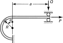
10.7. A square slender bar in the form of a quarter ring of radius R is fixed at one end (Fig. P10.7). At the free end, force P and moment Mo are applied, both in the plane of the bar. Using Castigliano’s theorem, determine (a) the horizontal and the vertical displacements of the free end and (b) the rotation of the free end.
10.8. The curved steel bar shown in Fig. 10.6 is subjected to a rightward horizontal force F of 4 kN at its free end and P = 0. Using E = 200 GPa and G = 80 GPa, compute the horizontal deflection of the free end taking into account the effects of V and N, as well as M. What is the error in deflection if the contributions of V and N are omitted?
10.9. It is required to determine the horizontal deflection of point D of the frame shown in Fig. P10.9, subject to downward load F, applied at the top. The moment of inertia of segment BC is twice that of the remaining sections. Use Castigliano’s theorem.
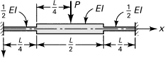
10.10. A steel spring of constant flexural rigidity is described by Fig. P10.10. If a force P is applied, determine the increase in the distance between the ends. Use Castigliano’s theorem.
10.11. A cylindrical circular rod in the form of a quarter-ring of radius R is fixed at one end (Fig. P10.11). At the free end, a concentrated force P is applied in a diametral plane perpendicular to the plane of the ring. What is the deflection of the free end? Use the unit load method. [Hint: At any section, Mθ = PR sin θ and Tθ = PR(1 – cosθ).]
10.12. Redo Prob. 10.11 if the curved bar is a split circular ring, as shown in Fig. P10.12.

10.13. For the cantilever beam loaded as shown in Fig. P10.13, using Castigliano’s theorem, find the vertical deflection δA of the free end.
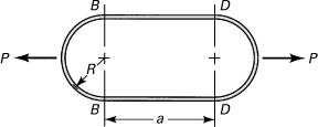
10.14. A five-member plane truss in which all members have the same axial rigidity AE is loaded as shown in Fig. P10.14. Apply Castigliano’s theorem to obtain the vertical displacement of point D.
10.15. For the beam and loading shown in Fig. P10.15, use Castigliano’s theorem to determine (a) the deflection at point C; (b) the slope at point C.
10.16. and 10.17. A beam is loaded and supported as illustrated in Figs. P10.16 and P10.17. Apply Castigliano’s theorem to find the deflection at point C.
10.18. A load P is carried at joint B of a structure consisting of three bars of equal axial rigidity AE, as shown in Fig. P10.18. Apply Castigliano’s theorem to determine the force in each bar.
10.19. Applying the unit-load method, determine the support reactions RA and MA for the beam loaded and supported as shown in Fig. P10.19.
10.20. A propped cantilever beam AB is supported at one end by a spring of constant stiffness k and subjected to a uniform load of intensity p, as shown in Fig. P10.20. Use the unit-load method to find the reaction at A.
10.21. A beam is supported and loaded as illustrated in Figs. P10.21. Use Castigliano’s theorem to determine the reactions.
10.22. Redo Prob. 10.19, using Castigliano’s theorem.
10.23. A beam is supported and loaded as shown in Fig. P10.23. Apply Castigliano’s theorem to determine the reactions.
10.24. Determine the deflection and slope at midspan of the beam described in Example 10.8.
10.25. A circular shaft is fixed at both ends and subjected to a torque T applied at point C, as shown in Fig. P10.25. Determine the reactions at supports A and B, employing Castigliano’s theorem.
10.26. A steel rod of constant flexural rigidity is described by Fig. P10.26. For force P applied at the simply supported end, derive a formula for roller reaction Q. Apply Castigliano’s theorem.
10.27. A cantilever beam of length L subject to a linearly varying loading per unit length, having the value zero at the free end and po at the fixed end, is supported on a roller at its free end (Fig. P10.27). Find the reactions using Castigliano’s theorem.
10.28. Using Castigliano’s theorem, find the slope of the deflection curve at midlength C of a beam due to applied couple moment Mo (Fig. P10.28).
10.29. The symmetrical frame shown in Fig. P10.29 supports a uniform loading of p per unit length. Assume that each horizontal and vertical member has the modulus of rigidity E1I1 and E2I2, respectively. Determine the resultant reaction RA at the left support, employing Castigliano’s theorem.
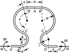
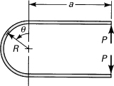
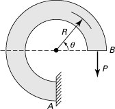
10.30. Forces P are applied to a compound loop or link of constant flexural rigidity EI (Fig. P10.30). Assuming that the dimension perpendicular to the plane of the page is small in comparison with radius R and taking into account only the strain energy due to bending, determine the maximum moment.
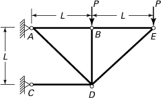
10.31. A planar truss shown in Fig. P10.31 carries two vertical loads P acting at points B and E. Use Castigliano’s theorem to obtain (a) the horizontal displacement of joint E; (b) the rotation of member DE.
10.32. Calculate the vertical displacement of joint E of the truss depicted in Fig. P10.32. Each member is made of a nonlinearly elastic material having the stress–strain relation σ = Kε1/3 and the cross-sectional area A. Apply the Crotti–Engesser theorem.
10.33. A basic truss supports a load P, as shown in Fig. P10.33. Determine the horizontal displacement of joint C, applying the unit-load method.
10.34. A frame of constant flexural rigidity EI carries a concentrated load P at point E (Fig. P10.34). Determine (a) the reaction R at support A, using Castigliano’s theorem; (b) the horizontal displacement δh at support A, using the unit-load method.
10.35. A bent bar ABC with fixed and roller supported ends is subjected to a bending moment Mo, as shown in Fig. P10.35. Obtain the reaction R at the roller. Apply the unit-load method.
10.36. A planar curved frame having rectangular cross section and mean radius R is fixed at one end and supports a load P at the free end (Fig. P10.36). Employ the unit-load method to determine the vertical component of the deflection at point B, taking into account the effects of normal force, shear, and bending.
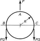
10.37. A large ring is loaded as shown in Fig. P10.37. Taking into account only the strain energy associated with bending, determine the bending moment and the force within the ring at the point of application of P. Employ the unit-load method.
Sections 10.8 through 10.11
10.38. Redo Problem 10.25, employing Castigliano’s first theorem. [Hint: Strain energy is expressed by
(P10.38)
where θ is the angle of twist and GJ represents the torsional rigidity.]
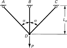
10.39. Apply Castigliano’s first theorem to compute the force P required to cause a vertical displacement of 5 mm in the hinge-connected structure of Fig. P10.39. Let α = 45°, Lo = 3 m, and E = 200 GPa. The area of each member is 6.25 × 10⁻⁴ m2.
10.40. A hinge-ended beam of length L rests on an elastic foundation and is subjected to a uniformly distributed load of intensity p. Derive the equation of the deflection curve by applying the principle of virtual work.
10.41. Determine the deflection of the free end of the cantilever beam loaded as shown in Fig. 10.14. Assume that the deflection shape of the beam takes the form
(P10.41)
where a1 is an unknown coefficient. Use the principle of virtual work.
10.42. A cantilever beam carries a uniform load of intensity p (Fig. P10.42). Take the displacement v in the form
(P10.42)
where a is an unknown constant. Apply the Rayleigh–Ritz method to find the deflection at the free end.
10.43. Determine the equation of the deflection curve of the cantilever beam loaded as shown in Fig. 10.14. Use as the deflection shape of the loaded beam
(P10.43)
where a1 and a2 are constants. Apply the Rayleigh–Ritz method.
10.44. A simply supported beam carries a load P at a distance c away from its left end. Obtain the beam deflection at the point where P is applied. Use the Rayleigh–Ritz method. Assume a deflection curve of the form v = ax(L – x), where a is to be determined.
10.45. Determine the midspan deflection for the fixed-ended symmetrical beam of stepped section shown in Fig. P10.45. Take v = a1x3 + a2x2 + a3x + a4. Employ the Rayleigh–Ritz method.
10.46. Redo Prob. 10.45 for the case in which the beam is uniform and of flexural rigidity EI. Use
(P10.46)
where the an’s are unknown coefficients.