Dynamic Discrete Dislocation Plasticity
Beñat Gurrutxaga-Lerma*; Daniel S. Balint†; Daniele Dini†; Daniel E. Eakins*; Adrian P. Sutton* * Department of Physics, Imperial College London, London, United Kingdom
† Department of Mechanical Engineering, Imperial College London, London, United Kingdom
Abstract
This chapter concerns with dynamic discrete dislocation plasticity (D3P), a two-dimensional method of discrete dislocation dynamics aimed at the study of plastic relaxation processes in crystalline materials subjected to weak shock loading. Traditionally, the study of plasticity under weak shock loading and high strain rate has been based on direct experimental measurement of the macroscopic response of the material. Using these data, well-known macroscopic constitutive laws and equations of state have been formulated. However, direct simulation of dislocations as the dynamic agents of plastic relaxation in those circumstances remains a challenge. In discrete dislocation dynamics (DDD) methods, in particular the two-dimensional discrete dislocation plasticity (DDP), the dislocations are modeled as discrete discontinuities in an elastic continuum. However, current DDP and DDD methods are unable to adequately simulate plastic relaxation because they treat dislocation motion quasi-statically, thus neglecting the time-dependent nature of the elastic fields and assuming that they instantaneously acquire the shape and magnitude predicted by elastostatics. This chapter reproduces the findings by Gurrutxaga-Lerma et al. (2013), who proved that under shock loading, this assumption leads to models that invariably break causality, introducing numerous artifacts that invalidate quasi-static simulation techniques. This chapter posits that these limitations can only be overcome with a fully time-dependent formulation of the elastic fields of dislocations. In this chapter, following the works of Markenscoff & Clifton (1981) and Gurrutxaga-Lerma et al. (2013), a truly dynamic formulation for the creation, annihilation, and nonuniform motion of straight edge dislocations is derived. These solutions extend the DDP framework to a fully elastodynamic formulation that has been called dynamic discrete dislocation plasticity (D3P). This chapter describes the several changes in paradigm with respect to DDP and DDD methods that D3P introduces, including the retardation effects in dislocation interactions and the effect of the dislocation’s past history. The chapter then builds an account of all the methodological aspects of D3P that have to be modified from DDP, including mobility laws, generation rules, etc. Finally, the chapter explores the applications D3P has to the study of plasticity under shock loading.
1 Introduction
Plasticity or plastic deformation of a crystalline material refers to the permanent, irreversible changes in the shape of the material when it is subjected to external loads. Because plasticity leads to permanent changes in the shape of a body, it is of great industrial and economic importance. This significance is dual. On one hand, it can be regarded as an undesirable effect that one must avoid. This would be the case of plastic deformation in metallic structures: the civil engineer or architect designing a bridge wants to ensure that, once built, and under the application of its service loads, the shape of the bridge remains unchanged; i.e., that it will not permanently change just as a result of a few automobiles running through it. In this case, the onset of plasticity defines the ultimate admissible strength of the structure, which has to be designed in such a way as to ensure that it never undergoes plastic deformation. This will require a proper understanding of the causes of plasticity, knowing where and how its onset occurs.
On the other hand, plasticity can be turned to one's own advantage. There are many applications where attaining a permanent deformation is not only desirable but explicitly sought after. This would be the case of manufacturing techniques such as extrusion, stamping, hot and cold rolling, or forging, where the material is subjected to external loads with the sole intent of permanently changing its shape to serve a new purpose, such as manufacturing thin metallic plates, thin wires, and extruded beams. In these cases, it is not only of interest for the engineers or metallurgists in charge to know when plasticity begins but also the means by which it progresses and the different parameters (temperature for instance) that affect it.
Thus, plasticity in metals arises as a physical phenomenon of huge industrial and economic relevance. This alone justifies its study and demarcates the most interesting features of plasticity, to wit, its onset and the conditions in which it is reached, and the conditions and parameters affecting its development.
Although by no means the sole way to study plasticity, one of the most enlightening ways to understand it is to focus on its microscopic causes. Plasticity in crystalline materials occurs predominantly through the generation and motion of dislocations in the crystalline lattice. Dislocations are linear crystalline defects that can be regarded as the dynamic agents of plastic deformation at the microscopic scale. They can be imagined as additional half planes of atoms that distort the otherwise perfect crystalline lattice, introducing mechanical strains that tend to oppose or balance the external loads. Dislocations can interact with each other and with other defects, such as point defects or interfaces, and react to the external loads by moving in order to minimize the free energy of the system. The study of dislocations as crystalline defects is usually called the Theory of Dislocations, a field that ranges from experimental imaging of dislocations and dislocation structures (vid. Whelan, 1975), through to mesoscale theory (vid. Hirth & Lothe, 1991) and modeling (vid. Bulatov & Cai, 2006; Kubin, 2013) of dislocations as the carriers of plasticity, all the way down to atomistic simulations that study the features of the crystalline structure that affect plastic flow (vid. Gumbsch & Gao, 1999b; Moriarty, Vitek, Bulatov, & Yip, 2002; Vitek, 1992).
The relationship between plastic deformation and the generation and motion of dislocations is both simple and challenging to address. In 1678, Robert Hooke revealed through his famous adage Ut tensio, sic vis [As the deformation, so the force], the results of the experiments he had carried out 18 years before: that, up to a certain point, crystalline materials behave elastically, there being a linear, reversible correspondence between the applied force and the resulting deformation. However, as Hooke himself noticed, above a certain threshold of force, the material stops behaving elastically and, as we now know, plasticity ensues. This threshold is commonly called the yield point, above which the material undergoes plastic (permanent) deformation. The theory of dislocations identifies the yield point as the value of stress at which dislocations begin to move, breed, and interlock. As the number of dislocations increases, mutual interactions become more likely, which tends to hinder their motion. This is reflected in a relative hardening of the material, which means that the material requires a higher external load to undergo the same amount of deformation as it would have had the material remained elastic.
The theory of dislocations also helps in understanding some of the factors that affect plastic deformation. For instance, crystalline materials are easier to deform at higher temperatures, a fact dislocation theory explains by showing that the mobility of dislocations is generally enhanced at higher temperatures. The effects of different crystalline structures, grain boundaries, or grain sizes are also explained, on a fundamental level, by the theory of dislocations. For further details, the reader is referred to Hirth and Lothe's classic book on the subject (Hirth & Lothe, 1991).
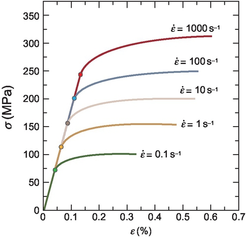
This chapter will focus primarily on one of the parameters that affect plastic flow, the strain rate, and how to study its effects using the theory of dislocations in a continuum level. Here, strain rate refers to the rate at which the material is deformed or loaded. Experimental observations of plastic deformation at different strain rates show that crystalline materials are usually harder at high strain rates, an effect similar to that of decreasing the temperature; this is shown in Fig. 2.1, whereby the yield point tends to increase with an increasing strain rate. The cause of this behavior is complicated.
Most studies of plasticity focus on low strain rates. A low strain rate signifies that the loads over the material are applied at a slow enough pace that the material's behavior can be characterized as quasi-static. In quasi-static analyses, the material is assumed to be in mechanical equilibrium at each instant in time. Under this assumption, as a result of the application of external boundary conditions, the material will evolve from one state of mechanical equilibrium to another. Most real-life situations where plasticity is present are well characterized as quasi-static. This includes physical processes such as ductile fracture and indentation, as well as structural design of car frames and other metallic structures, and manufacturing methods such as cold rolling. In fact, many applications, such high-speed forging, which are commonly regarded as “high strain rate” processes, are actually low strain rate in the context of plastic deformation.
In low strain rate plasticity (below ≈ 104 s−1), the material's plastic behavior is what is typically expected from a tensile stress–strain test, as shown in Fig. 2.1: up to a given value of stress (the yield point), the material behaves elastically; above the yield point, the material experiences plastic flow primarily as a result of the motion, generation, and interaction of dislocations. The main characteristic of plasticity in the low strain rate “regime” is that the yield point tends to increase (logarithmically) with the strain rate (Follansbee, Regazzoni, & Kocks, 1984), to wit, the material seems proportionally harder with an increasing strain rate. The “hardening” is small and can be characterized through the stress–strain curve so long as the effect of the strain rate is properly reflected, as shown in Fig. 2.1.
However, as depicted in Fig. 2.2, at strain rates of the order of 104–106 s−1, the material's yield point experiences a sudden upturn. This upturn in the yield point suggests that the kinetics of plastic flow of the material (i.e., the way dislocations are generated and move) undergo a fundamental change at high strain rates. Several attempts have been made to explain it. Follansbee et al. (1984) and Regazzoni, Kocks, and Follansbee (1987) proposed a change in the regime of motion of dislocations as a likely cause, progressing from a thermally activated motion to a drag-controlled motion. Regazzoni et al. went further, suggesting a possible change in the dislocation generation mechanisms. More recently, Fan, Osetsky, Yip, and Yildiz (2012) have attributed the upturn in the yield stress to the strain rate dependence of the activation stress in the motion of thermally activated dislocations. In turn, Agnihotri and Van der Giessen (n.d.) have associated the upturn with the rate dependence of the activation stress of Frank–Read sources of dislocation and reported a relatively small effect of dislocation drag.

The upturn is accompanied by a fundamental change in the loading regime, which becomes dynamic. Dynamic loads are transmitted throughout the material by mechanical waves traveling at a finite speed. In principle, all loads inside a material are transmitted by waves. Mechanical waves propagate in a solid at the speed of sound, which is about a few thousands of meters per second in a metal. The transmission of loads in solids can be much faster than the rate at which the loads themselves are applied. In that event, the material can be treated quasi-statically, and the transition between one mechanical state and the next can be imagined as a sequence of states of mechanical equilibrium. However, when the loads are applied at a high enough rate, comparable to the speed of sound, the traveling waves do not have time to propagate throughout the material on the timescale of the loading regime, leading to regions of the material that are loaded, while others are not. This highlights the importance of treating inertial effects in dynamic loading and presents mechanistic description of the material based on wave propagations.
The most characteristic example of dynamic loading is shock loading. Shock loads are high-intensity compressive loads characterized through a very high strain rate (at least above 106 s−1, commonly about 108–109 s−1). If one ignores plasticity for a moment, in shock loading the material will be loaded with a shock front: a single wave front that takes the material from the undisturbed unshocked state where1 P0 = 0 to the shocked state, sometimes called the Hugoniot state, where the pressure in the material takes a high value P1 (for most metals, at least a few gigapascals) with a corresponding compression ρ1 = 1/v1, where ρ and v are, respectively, the density and the specific volume.
Here, the strain rate ![]() refers to the rate with which the material is continuously loaded from the unshocked to the Hugoniot state. The shock front propagates with a finite speed, vfront. Thus, the strain rate can be conceived as the thickness dfront of the shock front, where
refers to the rate with which the material is continuously loaded from the unshocked to the Hugoniot state. The shock front propagates with a finite speed, vfront. Thus, the strain rate can be conceived as the thickness dfront of the shock front, where
where vfront is the shock front's own speed. If the shocked material displays a perfectly elastic behavior, this speed is the (longitudinal) speed of sound, c1). Otherwise, the nature of the speed of the shock front is less clear.
Shock fronts are typically characterized through the thermodynamic states of equilibrium they drive the material to and from, via the intensive parameters {P0, ρ0, T0, v0} (pressure, density, temperature, and speed, respectively) of the unshocked state and their shocked state counterparts {P1, ρ1, T1, v1}. Depending on the magnitude of the shock load, different shocked states can be reached. The locus of possible states of thermodynamic equilibrium that can be reached by shocking a given material forms the material's Hugoniot curve in the P−v plane. Figure 2.3 shows a typical Hugoniot curve of a crystalline material.
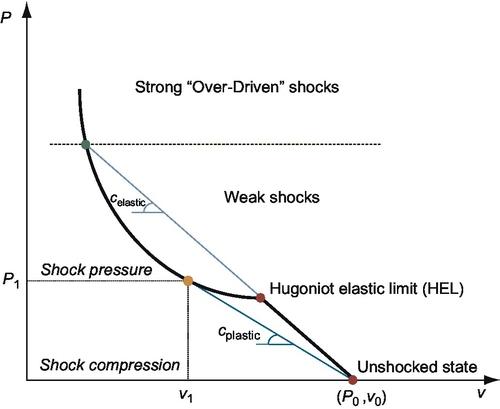
The Hugoniot curve can be thought of as a sui generis analogue of the stress–strain curve. As can be seen in Fig. 2.3, if the material behaves elastically, the Hugoniot curve is a straight line in the P–v plane. The material will behave plastically above the yield point that in this context is usually referred to as the Hugoniot Elastic Limit (HEL). Beyond the HEL, plastic flow ensues, which in this context is usually called plastic relaxation because the compressed material is “relaxed”—i.e., compressed comparatively less—as a result of plasticity.
Applying conservation of mass, energy, and linear momentum, it is possible to prove (Boslough & Assay, 1993) that the shock front's own speed relates the shocked and unshocked state as follows

Here,  happens to be the slope of the line that connects the unshocked state with the shocked state (vid. Fig. 2.3). This line is called the Rayleigh line (Meyers, 1994).
If the material is loaded below the HEL, then the Rayleigh line coincides point to point with the elastic Hugoniot curve. The corresponding speed that arises from applying Eq. (2.2) is the speed of sound, marked as celastic in Fig. 2.3. As shown there, above the HEL the slope of this line is typically lower than that of the elastic Hugoniot, at least up to a certain shocked state. Consequently, the speed of the shock front, marked as cplastic in Fig. 2.3, will be lower than the elastic speed of sound. The shocked states for which the slope of the Rayleigh line is lower than the elastic line's slope, form what is known as the weak shock regime; when it is higher than that, the resulting regime is called the strong shock or overdriven shock regime. The subsequent discussion will refer solely to weak shocks.
In the weak shock regime, the shock front displays a two-wave structure. Up to the HEL, the material sees a elastic precursor wave front propagating with the faster elastic speed of sound; above the HEL, the ensuing plastic front propagates with a slower speed that can be defined through Eq. (2.2). This “wave-splitting” phenomenon is depicted in Fig. 2.4.

Figure 2.4 also showcases the huge simplifications that are made when treating shock fronts thermodynamically. Because time is not a thermodynamic variable (Callen, 1985), all dynamic (i.e., time-dependent) effects are neglected, most fundamentally the strain rate. Consequently, in Fig. 2.4, the shock front has no thickness. A rather more realistic wave-split shock front profile is the one represented in Fig. 2.5, which represent experimental measurements of shock profiles in aluminum. Beyond displaying an elastic precursor and a plastic wave front, a real shock front profile such as this one is characterized through its strain rate—its thickness—and its continuity as opposed to Fig. 2.4.

Further simplifications have been introduced however. For instance, it would seem that the HEL in the Hugoniot curve must necessarily correspond to the quasi-static yield point. However, before discussing shock loading and high strain rate phenomena, it has already been noted that the yield point depends heavily on the applied strain rate, as shown in Fig. 2.2. Nothing in the Hugoniot curve's thermodynamic treatment captures this, at least a priori.
The Hugoniot analysis has nonetheless been presented here because it serves to highlight the new dimension that shock and high strain rate loading introduce in the study of the plastic behavior of materials. In the quasi-static behavior, mechanical properties arise globally—effects might be local, but the properties are the same everywhere. In the dynamic behavior, the material's mechanical properties express themselves locally at propagating wave fronts: the yielding response varies greatly with the applied stress, and this is highly localized at the shock front. Hence, material properties cannot be measured any longer using tensile test machines; rather, specific experimental setups such as gas guns or laser facilities are required, where the magnitude of the front can be chosen and the arising wave profiles properly monitored. This alone justifies the existence of Shock Physics as a predominantly experimental discipline devoted to the characterization of the dynamic behavior of materials under shock loading.
The splitting of the shock front into an elastic precursor and a plastic wave suggests that under shock loading, as in the static case, dislocation activity plays a fundamental role in the plastic relaxation process. However, this is not true as it might immediately seem. In the compressive loads that shock fronts impose, additional effects such as crystalline lattice compressions and release waves incoming from the boundaries contribute to the relaxation of the material (i.e., to its unshocking) as well. Other effects such as twinning and phase transformations are commonly present as well, and they too relax the shock front. However, for weaker shocks, and omitting twinning and phase transformations from any further discussion, dislocation activity has the upper hand in the plastic relaxation of crystalline materials under shock loading (J. Taylor, 1965; Meyers, 1994). Many macroscopic constitutive models of shock-loaded materials are nowadays physically motivated by considering dislocation activity at the shock front (vid. Ding & Asay, 2011; Ding, Asay, & Ao, 2010; Partom, 1984), and there is a considerable amount of experimental evidence showing the evolution of dislocation structures under shock loads of different intensities (Meyers, Jarmakani, Bringa, & Remington, 2009).2
The effect of dislocations at the front can be best apprehended by supposing a perfectly elastic infinitely wide plate. When it is shocked, there is only a strain normal to the shock front. The shock front propagates at a constant speed equal to the longitudinal wave speed throughout the material. The strain rate at a point is zero before and after the shock has passed through, and is nonzero only while the shock front is passing through that point. The work done by the shock is converted into elastic strain energy in the region of the sample that is compressed, and grows at the longitudinal speed of sound. As the shock front passes any point in the sample, the normal stress rises from zero to the same maximum value: there is no plasticity because there are no energy dissipation mechanisms. However, if dislocation activity is allowed to occur, one would expect for dislocations to either begin their motion or, if there were not any, to be created as the shock front loads the material. The dislocations that are created at and behind the shock front relax the elastic stresses created there by the shock front as it passes through; this process is equivalent to saying that their generation and subsequent motion is a dissipative mechanism that converts part of the shock front's energy into phonons (dissipation) and their own elastic self-energy, so that not all of the front's energy is spent in increasing the local strain energy anymore. Thus, dislocations give rise to the plastic wave that trails behind the elastic wave. Plasticity being caused by the motion and generation of dislocations, the shock front will mark the start of their motion and generation, thus being an area of great interest for studying dislocation mechanics.
With dislocations, one is able to offer qualitative explanations and predictions regarding the macroscopic response of the material by considering simple microscopic defects. However, to date it remains difficult to bridge the gap between what is essentially a microscopic theory of defects and plastic deformation itself, which commonly refers to the observed macroscopic response of the material. There are a number of factors that contribute to these difficulties. On one hand, dislocations are line defects. Therefore, they have many more degrees of freedom to move and interact with than, for instance, point defects; this makes their interactions with one another and with the medium challenging to compute. On the other hand, the number of dislocations existing in any material undergoing plastic deformation is exceedingly large, often reaching values of 1014 dislocations per m2—indeed, under shock loading one often expects dislocation densities above 1015–1016 dislocations per m2 (Meyers, 1994). Thus, the mathematical and numerical treatment of the macroscopic plastic deformation by considering the collective effect of each individual dislocation becomes challenging. Multiscale modeling of dislocations, which involves computer simulation techniques such as discrete dislocation dynamics or phase field modeling (Bulatov & Cai, 2006), is an attempt to bridge this gap.
The aim of this chapter is to study how plasticity and dislocation activity are different under shock loading compared to the plastic deformation and dislocation activity under quasi-static loading. In order to do so, this chapter will consider discrete dislocation dynamics as the method of choice, whereby dislocations will be treated as elastic defects that interact and move in a continuum, in an attempt to draw conclusions both as to their macroscopic effect and the result microscopic structures. Under shock loading, one should expect a bigger role of the dynamics and kinetics of the plastic flow of the material, whereby wave propagation takes the stage. Thus, the boundary conditions applied in shock loading are dynamic; they trigger propagating wave fronts and, consequently, the material's response has to be studied dynamically as well. This will affect the activity of dislocations themselves, which, as it will be elaborated upon, leads to an important drawback: most of the theory of dislocations, including all mesoscale methods of simulating plastic response through dislocation activity, are quasi-static. In this chapter, this drawback is overcome by introducing a novel methodology of discrete dislocation dynamics that accounts for the dynamics of dislocation activity as well as the material's.
This new method is called dynamic discrete dislocation plasticity (D3P), a method of discrete dislocation dynamics characterized through its treatment of the elastic fields of dislocations as time-dependent, elastodynamic, moving in an elastodynamic continuum. The method, originally proposed by Gurrutxaga-Lerma et al. (2013), stems as an extension of discrete dislocation plasticity (DDP). It is, therefore, a two-dimensional dislocation dynamics method that considers solely the activity of straight edge dislocations. This constitutes an oversimplification of major dislocation mechanisms such as cross-slip, but offers valuable insights in plane strain situations such as those expected in shock loading. Furthermore, it is to date the sole method of discrete dislocation dynamics that is fully time-dependent, dynamic. In fact, the time-dependent fields of dislocations produce a fundamental change of paradigm with respect to DDP and, in general, dislocation dynamics methods: all dislocations interactions with one another and with the medium will be based on a retardation principle, whereupon the fields require some time to propagate from one point to another, radically changing the inner workings of the method. This feature, alongside many others, will be discussed in detail in the following pages.
Thus, the chapter is structured as follows. In Section 2, a review of dislocation dynamics with a particular focus to two-dimensional models is offered. As suggested above, most of these methods are not adapted to simulating dynamic loads such as shock waves and cannot capture the effects that the expected fast moving dislocations should display according to dislocation theory. Thus, Section 3 reviews the fundamental understanding of dynamic effects in traditional dislocation theory. However, the latter overlooks problems arising when the interactions of many dynamic dislocations are considered at the same time; Section 4 will show that a fully elastodynamic treatment of the dislocation fields is required because, otherwise, causality is broken. As a result, in Section 5, the elastodynamic fields of an injected, nonuniformly moving edge dislocation will be derived. These solutions constitute the foundation over which D3P is built. The most important features of this solution are discussed in detail in Section 7; the many subtleties related to their numerical implementation are explained in Section 6. Finally, this chapter explains the necessary methodological rules of D3P in Section 8 and finishes in Section 9 with some numerical applications of the method, showing what a D3P simulation looks like. Section 10 concludes with a summary the main points of this method.
2 Discrete dislocation dynamics
The aim of discrete dislocation dynamics is to simulate plasticity as the result of the collective motion of individual dislocations (Gurrutxaga-Lerma et al., 2013). There is not a single technique of discrete dislocation dynamics (DD), but a varied family of methods that have several characteristic in common.
In DD, dislocations are modeled as individual Volterra singularities in an elastic continuum, and plasticity arises as a result of their generation and motion. Long-range interactions between dislocations are accounted for through the overlapping elastic fields of individual dislocations. Short-range interactions such as annihilations, pinning by obstacles, or collisions between dislocations are modeled through constitutive rules that are applied when the dislocations involved meet a series of specific criteria (e.g., coming within a certain distance of one another, reaching a threshold value of stress).
Further constitutive rules are commonly needed. Mobility laws are defined to describe the motion of the dislocations as a result of an applied external stimulus. These are necessary to allow the microstructure of dislocations to evolve as a result of the external boundary conditions and the mutual interactions between the dislocations themselves. Dislocation generation rules are usually defined as well. These rules describe the conditions under which new dislocations are injected into the system and the manner in which this process occurs. This may include the definition of Frank–Read sources which generate a new dipole when a threshold stress is overcome, or the conditions by which dislocation loops expand and cross-slip. The specific details depend on the precise nature of the method of dislocation dynamics used.
Nevertheless, the general characteristic of dislocation dynamics methods are those outlined above: dislocations are modeled as discontinuities in an elastic continuum, where they interact with one another and with the medium through their elastic fields, and they are allowed to move and react in their specific slip planes using constitutive rules. Plasticity then arises as the result of their generation, motion, and interactions.
2.1 Methods of dislocation dynamics
DDP refers to a particular variant of discrete dislocation dynamics.3 As outlined above, DD methods share a common aim: the simulation of the motion of individual dislocations and the evolution of the dislocation microstructure as a way of studying plastic flow. DDP is the application of that principle in two dimensions. This limits the scope of the method to straight, infinite edge dislocations alone.
In DDP, each dislocation line is perpendicular to the 2D medium considered; dislocations are assimilated to point-like particles that move in their respective slip planes. Their motion can be halted by point-like obstacles, and they are generated by point-like Frank–Read sources. Figure 2.6 depicts the main elements of a DDP simulation. This simplification has the obvious shortcoming of neglecting effects mediated by screw dislocations (forest hardening, cross slip, etc.). But at the same time, it provides a simple, computationally cheap and robust methodology able to tackle large systems with flexible boundary conditions.

DDP was introduced by Van der Giessen and Needleman in 1995 (Van der Giessen & Needleman, 1995) as a departure from previous two-dimensional dislocation models (Amodeo & Ghoniem, 1990a, 1990b; Bacon, 1967; Foreman, 1967; Gulluoglu & Hartley, 1992, 1993; Gulluoglu, Srolovitz, David, LeSar, & Lomdahl, 1989; Lépinoux & Kubin, 1987). The key feature of DDP is its handling of the boundary conditions using linear superposition following the original proposal by Lubarda, Blume, and Needleman (1993). As shown later in Fig. 2.38, the original problem consists of a set of boundary conditions and dislocations; the latter are strong discontinuities in a finite-sized medium. The resulting elastic problem is highly incompatible, so the numerical treatment of the whole problem is commonly extremely challenging, and its analytical treatment is out of the question. By invoking the linear superposition principle, the problem is divided into two more tractable systems. First, an infinite plane with dislocations is considered; this is very advantageous because the analytic solution of the elastic fields of dislocations is known, so mutual interactions between dislocations can be easily treated. Second, a finite-sized problem where the boundary conditions are applied is considered. This problem may be solved using numerical methods such as the finite element method or the boundary element method. Linear superposition is satisfied by calculating the tractions and displacements due to the dislocation's elastic fields over the mapped body surface in the infinite plane, and applying them with reversed sign in the finite-size problem. This ensures great flexibility in the handling of boundary conditions and an affordable computational cost for the simulations. Hereafter, the auxiliary finite-size boundary value problem will be referred to as the “boundary value” problem.
DDP has been used to study many dislocation-mediated problems, most typically finite-size problems where plane strain conditions apply and cross-slip is not expected to be a major mechanism: size effects in plastic flow (Balint, Deshpande, Needleman, & Van der Giessen, 2006; Nicola, Van der Giessen, & Needleman, 2003), geometrical effects (Romero, Segurado, & Lorca, 2008), fracture mechanics (Deshpande, Needleman, & Van der Giessen, 2003; O'Day & Curtin, 2005; Van der Giessen, Deshpande, Cleveringa, & Needleman, 2001), crack growth (Cleveringa, Van der Giessen, & Needleman, 2000), fatigue (Deshpande, Needleman, & Van der Giessen, 2002), creep (Ayas, van Dommelen, & Deshpande, 2014), etc. Thus, despite the obvious shortcoming, DDP still offers valuable insight into many problems.
The obvious shortcomings of 2D models can be overcome using three-dimensional “Dislocation Dynamics” (3D DD) (q.v. Bulatov & Cai, 2006; Ghoniem & Sun, 1999; Kubin & Canova, 1992; Schwarz, 1999; Zbib & Diaz de la Rubia, 2002). In this method, dislocations are modeled as closed three-dimensional loops in a continuum, so that dislocations of all characters are modeled. The inherent complexity of this technique lies in the necessity to discretize loops into discrete segments. As such, dislocations in the 3D continuum are represented as closed loops that, even after being discretized, have a very large number of degrees of freedom and possible interactions to allow for an easy numerical treatment. In 3D DD, the expressions of the dislocation loops' elastic fields are usually calculated numerically (Bulatov & Cai, 2006; Zbib & Diaz de la Rubia, 2002) at a significantly greater computational expense than in DDP. This typically limits the size and runtime of the simulations. Further problems with dislocations at the boundaries usually limit simulations to the use of periodic boundary conditions (Zhou, Bulent Biner, & LeSar, 2010). Thus, 3D dislocation dynamics methods offer a much more complete picture of dislocation activity at the cost of increased complexity and computational cost. Despite the challenges, 3D DD has nevertheless been used for the study of the effects, interactions, and structure of forests of dislocations with great success (Bulatov & Cai, 2006; Kubin, 2013).
3 Dynamic effects in the motion of dislocations
The simulation of plasticity at high strain rates using methods of dislocation dynamics has been attempted previously. Shehadeh, Zbib, and Diaz de la Rubia (2005), Bringa, McNaney, and Remington (2006), and Shehadeh (2012) have used a three-dimensional formulation of dislocation dynamics for the study of shock compression of solids. Their formulation, called multiscale dislocation dynamics plasticity (MDDP), was an extension of the general MDDP formulation previously presented by Zbib and Diaz de la Rubia (2002).
This formulation, like all other DD methods both in 3D and 2D (including DDP), is quasi-static. The elastic fields of both the dislocations and the external fields are time independent, i.e., elastostatic. Time is introduced to allow the dislocation structure to evolve, but it is not a field variable; thus, in DD methods, the elastic fields of a moving dislocation are propagated instantaneously. This assumption enables the stress field at an instant in time to be evaluated by considering the static elastic fields of the dislocations at their current positions, which is reasonable as long as the representative speeds of the system (the speeds of dislocations or of the boundary conditions, for instance) are a small fraction of the elastic transverse speed of sound. Expressions for the elastostatic fields of straight dislocations can be found in Hirth and Lothe (1991); in Mura (1982), a detailed analysis and derivation of the latter as well as a complete framework for the calculation of the fields of arbitrary closed dislocation loops are given.
However, in quasi-static approaches, the time-independent elastic medium is unable to produce dynamic feature such as a propagating shock front. Shehadeh and coworkers recognized this shortcoming and modified the medium's elastic field to make it time dependent, i.e., elastodynamic. In their approach, the elastic fields of dislocations are left unchanged, i.e., time independent. It will be discussed below that a consequence of this “hybrid” dynamic–quasi-static approach is that causality is violated.
Furthermore, particularly for high strain rate shock-loading situations, it is conceivable that the speed of dislocations themselves becomes a significant fraction of the transverse speed of sound. This is in fact an old litany of dislocation theory, usually expressed as at high strain rates, the dislocation velocity will be closed enough to the speed of sound that dynamic effects might be relevant (cf. Coffey, 1994; Gilman, 1969; Hirth & Lothe, 1991). Roos, De Hosson, and Van der Giessen (2001a, 2001b) recognized this fact and extended the two-dimensional DDP methodology to account for some of the classical dynamic effects in dislocation motion for materials sheared at high strain rates. These classical dynamic effects are discussed in the following section. Unfortunately, they overlook a fundamental piece of physics, as a result of which causality is violated as well.
3.1 Elastic fields of a preexisting, uniformly moving edge dislocation
The classical dynamic effects in dislocation motion refer to the changes in the form of the elastic fields of dislocations as a result of their motion, usually at hight speeds, compared to their elastostatic counterparts. The first analysis of these effects was introduced by Frank (1949) and Eshelby (1949b). In 1949, they analyzed the motion of a straight screw (Frank, 1949) and edge (Eshelby, 1949b) dislocations moving with constant speed in a rectilinear fashion. His work was expanded by Weertman (1967). Below, the same kind of analysis is presented for an edge dislocation, as originally described by Mura (1982).
Consider a uniformly gliding edge dislocation, where v is its velocity in the x1 direction, which therefore corresponds to the direction of the Burgers vector as well. The edge dislocation is a moving discontinuity that can be expressed as
where H(·) is the Heaviside function and δ Dirac's delta. Hence, this denotes a distortion in the x2 direction, where the dislocation line is. Notice that this boundary condition presupposes that the dislocation has been moving with speed v since t → −∞ to. The importance of this will become clear later.
Fourier transforming Eq. (2.3),
where ![]() .
.
The uniformly moving displacement field is given by Mura's formula (Mura, 1982) that
where the dynamic Green's tensor is

and where in this case ![]() . Usually, its determinant is called D and the cofactors Nij.
. Usually, its determinant is called D and the cofactors Nij.
For the isotropic case, it is found that
Thus,

This can be integrated to get


where  and
and ![]() are the longitudinal and transverse Mach number, and B ≡ b1 is the Burgers vector.
are the longitudinal and transverse Mach number, and B ≡ b1 is the Burgers vector.
The stress fields can be then obtained from Hooke's law, where
Thus,


and σ33 = ν(σ11 + σ22) as per plane strain requirement. Equations (2.8)–(2.10) and (2.12)–(2.14) are the ones Roos, De Hosson, and Van der Giessen (2001a) employed in their DDP model in place of the usual expressions for the elastostatic fields of dislocations (vid. Hirth & Lothe, 1991).
Figure 2.7 shows the shape of the σ12 stress component calculated in Eq. (2.12). It can be seen that the field tends to contract in the direction of motion as the dislocation's speed approaches the transverse speed of sound, i.e., as Mt → 1. Because the contraction of the elastic fields evokes the Fitzgerald contraction in the relativistic motion of electric charges, the regime of velocities of a dislocation at which this becomes a noticeable phenomenon is usual called the relativistic regime.

From the moment this contraction was noted, “suspicion” was raised that at high speeds, the change in the shape of the fields could play a significant role in the global response of the material (Gillis & Kratochvil, 1970). In that light, approaches such as that by Roos et al. (2001a); Roos, De Hosson, and Van der Giessen (2001b) are justified. After all, if one expects the speed of the dislocations to reach a significant fraction of the speed of sound, elasticity shows that the elastic fields of dislocations depart dramatically from the elastostatic Mt = 0 case.
3.2 Relativistic effects
Considering relativistic effects in dislocation motion reveals some surprising results. When the dislocation's speed reaches the transverse speed of sound, the field diverges. This can be seen in Eq. (2.12), and it happens for all other components of stress and displacement (vid. Eqs. 2.13 and 2.14). Thus, elasticity predicts that the elastic fields of a uniformly moving straight dislocation diverge at the transverse speed of sound.
Consider the elastic energy per unit volume,
Recall that  , for the linear isotropic case. Therefore,
Operating and contracting

Expanding it for plane strain

As in the quasi-static case, this energy density will be integrated over a disc of radius R − rc, so it is best to transform U to spherical polar coordinates, whereby x1 − vt = r cos θ and x2 = r sin θ. The elastic energy will be

where rc is the radius of the core of a dislocation and R the outer radius.
Substituting the expressions for the stress field above, and after some operations, one finally obtains

Figure 2.8 shows the evolution of the total elastic energy E of a uniform edge dislocation with respect to Mt = v/ct. Clearly, if σij diverges at Mt = 1, so does U and, concurrently, E. Furthermore, from Eq. (2.20), it is clear that the elastic energy of the dislocation increases as v → ct. Thus, there seems to exist an infinite elastic energy barrier when v = ct (Weertman, 1981).

The divergence of the elastic fields of dislocations and, consequently, of the elastic energy suggests that dislocations will never be able to move supersonically.4 This was nonetheless questioned by Gumbsch and Gao (1999a), whose molecular dynamics (MD) simulations of fast moving dislocations in tungsten showed the possibility of transonic and supersonic dislocations. As far as the authors know, experimental evidence of dislocations moving above the transverse speed barrier is still lacking, other than for two-dimensional plasma crystals (Nosenko, Zhdanov, & Morfill, 2007). However, since 1999 a great number of MD simulations have shown transonic dislocations for a wide number of materials (Li & Shi, 2002; Marian & Caro, 2006; Olmsted, Hector, Curtin, & Clifton, 2005; Tsuzuki, Branicio, & Rino, 2008).
3.3 Core instabilities and kinematic generation
Recently, Markenscoff and Huang (2008, 2009) have proposed that the failure of elasticity to explain these observations might be caused by the modeling of the dislocation's core as a Volterra discontinuity, and have argued that at high speeds the dislocation core tends to contract and should therefore be modeled accordingly.
This is in line with several remarks previously made in dislocation theory. Eshelby (1949b) and Weertman (1961) noticed that, in Eq. (2.12), in the direction of motion—i.e., the slip plane, x2 = 0—the magnitude of the shear stress component σ12 tends to decrease as the dislocation's speed increases, and that it cancels out and reverses in sign when it reaches the Rayleigh wave speed.5 Eshelby (1949b) employed a Peierls–Nabarro model to study the core of the uniformly moving edge dislocation, and reported that the width of the core vanished at the Rayleigh wave speed. He suggested that the Rayleigh wave speed was therefore the true limiting speed of dislocations, despite the actual divergence of the fields taking place at the higher transverse speed of sound.
Weertman (1961) rejected Eshelby's suggestion by pointing out that above the Rayleigh wave speed the dislocation's core regains its width. He also suggested that, because of the reversal in the sign of the field, above the Rayleigh wave speed like-signed dislocations in the same slip plane could attract rather than repel each other, and vice versa, forming superclusters of “double” dislocations (vid. Fig. 2.9A). Upon examining the energetics of such phenomenon, Weertman concluded that not only were those superclusters energetically possible, but that reactions such as those shown in Fig. 2.9B, leading to the dissociation of a single dislocation into a tripole formed by a double dislocation, and an unlike-signed dislocation, are possible. The latter process has been called kinematic generation of dislocations (Hirth & Lothe, 1991).

Hirth and Lothe (1991) identified this as an instability of the core of the dislocation. Kinematic generation of dislocations remains a largely unexplored area; however, it has been described in some MD simulations, notably by Weinee and Pear (1975), Schiotz, Jacobsen, and Nielsen (1995), Koizumi, Kirchner, and Suzuki (2002), and Tsuzuki, Branicio, and Rino (2009). In the latter two, the dissociation was not identified as such, but core instabilities were reported nonetheless. Other MD simulations of dislocations moving in the relativistic regime have reported core instabilities as well. For instance, Gumbsch and Gao (1999a) reported a contraction in the width of the dislocation's core as the dislocation lowered its speed below the transverse speed of sound. Olmsted et al. (2005) reported the existence of dislocations transversing the shear barrier that, in the transonic regime, became unstable and dissociated into partials.
The contraction of the width of the core was also explored by Jin, Gao, and Gumbsch (2008), who connected it to the Rayleigh wave speed, reporting significant energy losses in the motion of dislocations moving with speeds close to it. They went further to identify the Rayleigh wave speed as the limiting speed of dislocation motion. Several elastodynamic analyses of dislocation motion have suggested the same, e.g., Hirth and Lothe (1991), Weertman (1961), and Brock (1982).
Whether or not a core instability occurring around the Rayleigh wave speed could lead to an additional mechanism of generation of dislocations, or whether other effects such as dissociations are possible, remains largely an unanswered question. As said, simulations done in this area tends to point toward an unstable dislocation core at the shear wave barrier, as suggested by Eshelby and Weertman. However, a better understanding of what this implies would be very valuable, as it would help determine the likelihood with which dislocations become transonic or, otherwise, whether or not the material prefers, in general, to generate more dislocations through kinematic generation rather than accelerate the existing ones above the shear wave barrier.
4 Dislocation dynamics and causality
Despite including dynamic effects either by means of modifying the boundary conditions (as done by Shehadeh, 2012; Shehadeh et al., 2006, 2005) or by altering the fields of dislocations to account for the way they change at higher speeds (as done by Roos et al., 2001a, 2001b), there is a fundamental piece of physics that has been hitherto overlooked.
In the same way the shock front itself propagates with a well-defined, finite speed, one can expect that the dynamic fields of dislocations propagate at the speeds of sound. As commented in Section 3.1, the solution offered by Eshelby (1953) in Eqs. (2.8)–(2.10) and (2.12)–(2.14) refers to the motion of an edge dislocation that had been moving with speed v since t → −∞. Unsurprisingly, information about the fact that the dislocation is moving with speed v has already reached all points in the infinite medium at time t > 0. Hence, the Eshelby solution is a steady-state solution.
This does not reflect reality. In truth, a dislocation is created at some point of the crystalline lattice and at a given instant in time, and it then begins its motion, most likely nonuniformly. Information about its past whereabouts will reach any given point in the medium at the corresponding speeds of sound, which are high but finite. So if the process driving the dislocations is as fast as, say, the rise of a shock wave, neglecting the finite propagation time of the dislocation's fields results in a breach of the causality of the model in question.
To illustrate this point, consider the proof-of-concept simulation reported by Gurrutxaga-Lerma et al. (2013), where the DDP methodology was adapted in such a way that the elastostatic fields of dislocations are retained, but the boundary value problem was modified so as to allow the medium to propagate a shock front. Thus, the model remains quasi-static with respect to the elastic fields of dislocations, as done by Shehadeh and coworkers.
As shown in Fig. 2.10, a 40 × 20-μm 2D block is shocked with a high-pressure dynamic load under plane strain conditions. The intention is to mimic a high-velocity impact between a pair of thin plates, as it is commonly done experimentally (Meyers, 1994). Notice that the aspect ratio of the sample considered here is not representative of empirical reality, where the vertical dimension is usually at least one order of magnitude larger than the horizontal one.

To simulate the dynamic loading of the 2D block, the left surface was loaded with a constant uniaxial stress at t = 0 that excites an elastodynamic wave front propagating through the solid. The upper and lower surfaces were defined as traction-free surfaces, whereas over the right surface a reflective boundary condition was applied. A commercial finite element package, ABAQUS, was coupled to the DDP code via Python scripting, and an explicit solver was used for the solution of the associated elastodynamic, finite-size problem. As in usual DDP simulations, the fields of dislocations were assumed to be elastostatic and therefore to propagate instantaneously.
The elastic parameters of aluminum were used6 in the simulation. Slip planes were oriented at ±45° and 90° to the direction of impact and spaced by 100 Burgers vectors. A random population of sources and obstacles was assumed in the slip planes, with a density of ρs = 100 μm−2. The motion of dislocations was assumed to be overdamped, following a viscous drag mobility law of the form v = Bτ/d, with a viscous drag coefficient d = 10−5 Pa s. The speed of dislocations was capped at the transverse speed of sound. A forward Euler integration scheme was used, with a dynamic time-step that limited dislocation motion to 1 nm per time step. Low-intensity Frank–Read sources alone were considered, with a strength of 100 ± 10 MPa taken from a Gaussian distribution; the strength of obstacles was set at 100 MPa.
The breach in causality mentioned above is made clear in Fig. 2.11A and B, which show the positions of the shock front and the corresponding dislocation microstructures at t = 0.9 and 2 ns, respectively. Dislocations are seen to nucleate ahead of the front as a result of the stress fields originating from the dislocations generated behind the front. Because of the quasi-static approximation, the elastic fields of dislocations are transmitted throughout the sample at the instant the dislocations are created behind the front. This is completely unphysical and is a direct consequence of the quasi-static assumption. In reality, these stress fields would take a finite time to be propagated, and therefore, it would not be possible to activate dislocation sources until the elastic front has reached them, i.e., plastic deformation cannot be propagated faster than elastic deformation.


Presumably, this breach in causality has further effects other than triggering nucleation ahead of the front. For instance, dislocations will interact with one another instantaneously, and they will influence the boundaries instantaneously as well. Thus, even if they had not triggered nucleation ahead of the front (say, by neglecting stress fields of dislocations behind the front on sources ahead of the front), the use of quasi-static DDP would still produce questionable results.
5 The dynamic fields of dislocations
Figure 2.11A and B indicates that causality can be satisfied only by solving the elastodynamic equations for the generation, annihilation, and motion of dislocations. In this section, the elastodynamic solution for the fields of an injected (created) nonuniformly moving straight edge dislocation is derived. This solution, originally proposed by Markenscoff and Clifton (1981), Gurrutxaga-Lerma et al. (2013), describes the fields in terms of elastic wave perturbations propagating at the speeds of sound. By introducing this solution into DDP, causality is observed in DDP at any rate of loading. However, the elastodynamic solutions here describe more than that; as it will be argued, interactions change to be based on a retardation principle. This causes a fundamental change in the usual paradigm of dislocation dynamics, leading to a new methodology that, because it arises as the elastodynamic extension of DDP, is called Dynamic Discrete Dislocation Plasticity.
5.1 Governing equations
In isotropic elastodynamics, the governing equation is the equation of conservation of linear momentum, also known as the Navier–Lamé equation (Eringen & Suhubi, 1975; Landau & Lifshitz, 1986):

where a repeated index denotes summation, Λ and μ are Lamé's first and second constants, and ρ is the density of the medium; ui is the ith component of the elastic displacement vector, a function of position and time; ui,j denotes the first partial derivative of ui with respect to xj, where x1 ≡ x, x2 ≡ y, x3 ≡ z are Cartesian coordinates.
The Navier–Lamé equation (Eq. 2.21) can be separated into two separate wave equations by expressing the displacement field as the sum of the gradient of a scalar potential and the rotational of a vectorial potential (Eringen & Suhubi, 1975; Landau & Lifshitz, 1986). In the (x,z) plane under plane strain conditions, with uy = 0 and ∂/∂y() ≡ 0 this process results in two wave equations for the scalar potentials ɸ = ɸ(x, z, t) and ψ = ψ(x, z, t):

and
where  ,
, ![]() are the slownesses of sound, cn is the “longitudinal” wave speed
are the slownesses of sound, cn is the “longitudinal” wave speed ![]() , and ct is the “transverse” wave speed
, and ct is the “transverse” wave speed ![]() .
.
The components of the displacement in terms of the scalar potentials are

and

From Hooke's law, it also follows that


Thus, any isotropic, first-order elastodynamic problem in plane strain results in the linear superposition of two separate, independent monochromatic waves (Landau & Lifshitz, 1986), i.e., the longitudinal and transverse waves.
Having defined the governing equation, one still needs to solve them for a specific set of boundary conditions. In this case, these boundary conditions must describe the injection and motion of a straight edge dislocation. Here, the method introduced by Markenscoff and Clifton (1981) is followed. Markenscoff and Clifton obtained the solution for a preexisting straight edge dislocation moving at a nonuniform speed. The solution method itself was previously developed by Markenscoff (1980) for the nonuniform motion of a screw dislocation. In parallel, Brock (1982) produced an equivalent solution to that of Markenscoff and Clifton for a preexisting straight edge dislocation moving at a nonuniform speed. Based on Markenscoff's procedure, Jokl, Vitek, McMahon, and Burgers (1989) solved the injection of a static (nonmoving) screw dislocation. Gurrutxaga-Lerma et al. (2013) used the same procedure to solve for the injection of a static edge dislocation and complete the formulation for the injected, nonuniformly moving straight edge dislocation.
The general procedure is as follows. Consider an infinite straight edge dislocation moving in the x direction, whose line is in the direction of the y-axis (vid. Fig. 2.12). Its position with respect to the origin at a given instant in time t is defined by a piecewise continuous function l(t), called the past history function. This function will store all the past positions of the dislocation line up to the current time step, hence the name.

The boundary conditions to be satisfied by Eqs. (2.22) and (2.23) can be described as the linear superposition of two different contributions, as shown in Fig. 2.13:

i. The injection contribution. This contribution describes the creation of a nonmoving edge dislocation with Burgers vector ![]() at time t = 0:
at time t = 0:
ii. The mobile contribution. This contribution describes the nonuniform motion of an existing edge dislocation dipole where one of the dislocations remains quiescent at the origin, and the other begins to move nonuniformly (vid. Fig. 2.13). The solution to this problem was obtained by Markenscoff and Clifton (1981):
Here, H(x) is the Heaviside step function.
5.2 The elastic fields of an injected, nonuniformly moving straight edge dislocation
In order to ensure that the normal stress is zero on the slip plane due to the injected, nonuniformly moving dislocation, a further boundary condition is introduced
5.2.1 Solution procedure
Here, the elastodynamic fields of the injected nonuniformly moving dislocation are solved employing the Cagniard–de Hoop technique (Cagniard, 1939; de Hoop, 1960). This technique involves the successive application of Laplace integral transforms to the governing equations and the boundary conditions, to first solve the problem in this reciprocal space. The Cagniard–de Hoop technique then specifies the way to perform the inversion of the solution back to the real space.
Hence, first define the following Laplace transform in time and bilateral Laplace transform in x:
and

Notice that in Eq. (2.36), s appears in the exponential as a scaling factor for convenience.
These transforms are applied successively to both the boundary conditions and the governing equations. Thus, assuming that at t = 0 the dislocation is quiescent, the governing Eqs. (2.22) and (2.23) are transformed into
where α2 = a2 − λ2, and

where β2 = b2 − λ2.
The transformed governing equations, Eqs. (2.37) and (2.38), are second-order differential equations the solutions of which can immediately be found:
Here, C(λ, s) and C′(λ, s) are integration constants.
The value of these integration constants is determined by satisfying the transformed boundary conditions for each of the contributions. As said, in this problem, two separate boundary problems must be solved: the injection contributions defined by Eq. (2.32) and the mobile contributions defined by Eq. (2.33). The latter case was solved by Markenscoff and Clifton (1981), whereas the former was solved by Gurrutxaga-Lerma et al. (2013). In both cases, the subsequent solution procedure is the same. For simplicity, here the solution procedure for the injection contribution alone shall be described.
Once the governing equations are transformed and solved, the values of C(λ, s) and C′(λ, s) for the injection contribution are obtained by transforming the boundary condition given in Eq. (2.32). The following expressions are then obtained:

These are the transformed potentials, the inversion of which leads to the final solution, in this case for the injection contributions. The inversion of the transformed potentials can be directly obtained employing the Cagniard–de Hoop technique (Cagniard, 1939; de Hoop, 1960). However, it leads to a double convolution integral of difficult solution. Instead, it is simpler and more enlightening to perform the inversion for each component of stress and displacement.
Here, the procedure is illustrated for the shear component of stress, σxz:

Applying the successive Laplace transforms defined above over Eq. (2.43), it is found that
The transformed potentials are given by Eqs. (2.41) and (2.42), so substituting

There are clearly two separate components, one depending on Ψ representing transverse excitations and one depending on Φ representing longitudinal excitations. Each term must be inverted separately. Consider for instance the longitudinal term in Eq. (2.45):

In the Cagniard–de Hoop technique, the inversion is performed by applying the inverse Laplace transforms in time and space described above in reverse order. The inverse bilateral Laplace transform is defined by the Bromwich integral
The scaling factor s in the integrand is necessary for consistence with the definition of the bilateral Laplace transform in time that bears it in the kernel of the transformation.
Apply this integral to Eq. (2.46)

The Cagniard–de Hoop technique specifies here that the Cagniard form of this integral must now be found. The Cagniard form refers to rewriting Eq. (2.48) as a forward Laplace transform by making a suitable change of integration variable and, concurrently, of the integration path. Here, the following change of integration variable can be introduced
where τ ≥ 0. The new variable τ can be expressed as
It follows that λ and α are with respect to τ:
where r2 = x2 + z2.
The change of variable allows to rewrite the exponential function in Eq. (2.48), e−s(αz−λx), as e−sτ, which makes Eq. (2.48) approach the desired Cagniard form. However, the integration path in λ, formerly the Bromwich contour, must adequately be transformed as well. The contour of integration in the original λ plane is a Bromwich contour along the imaginary λ axis. Equation (2.51) provides the form of λ with respect to the new integration variable τ, which is in the form of branches of hyperbolas. From Eq. (2.51), it is noticed that upon changing variable to τ, the Bromwich contour can be distorted into a hyperbolic path as shown in Fig. 2.14. Indeed, invoking Cauchy's theorem and Jordan's lemma (Markenscoff & Clifton, 1981), the integral in the λ plane alongside the Bromwich contour is seen to be equivalent to the one in the same λ plane along the hyperbola in Fig. 2.14. The latter corresponds to an integral in the τ plane between τ = ra and τ → ∞.

Hence, the Cagniard form of the integral in Eq. (2.48) is found:

where H(τ − ra) is a Heaviside function, and τ − ra has the form of a retarded time.
The Cagniard–de Hoop technique is extremely useful because, upon applying now the inverse Laplace transform in time,

it can be clearly seen that because the inverse Laplace transform is applied over an expression written in the form of a forward Laplace transform, the solution is the integrand itself:
Employing Eq. (2.51), one can substitute in the equation above and find the value of that imaginary part, to get.

The same can be done for the rest of the terms and components. The results are summarized in Table 2.1.
Table 2.1
The Elastic Fields of an Injected Static Straight Edge Dislocation
|
|
|
|
|
|
|
|
|
|


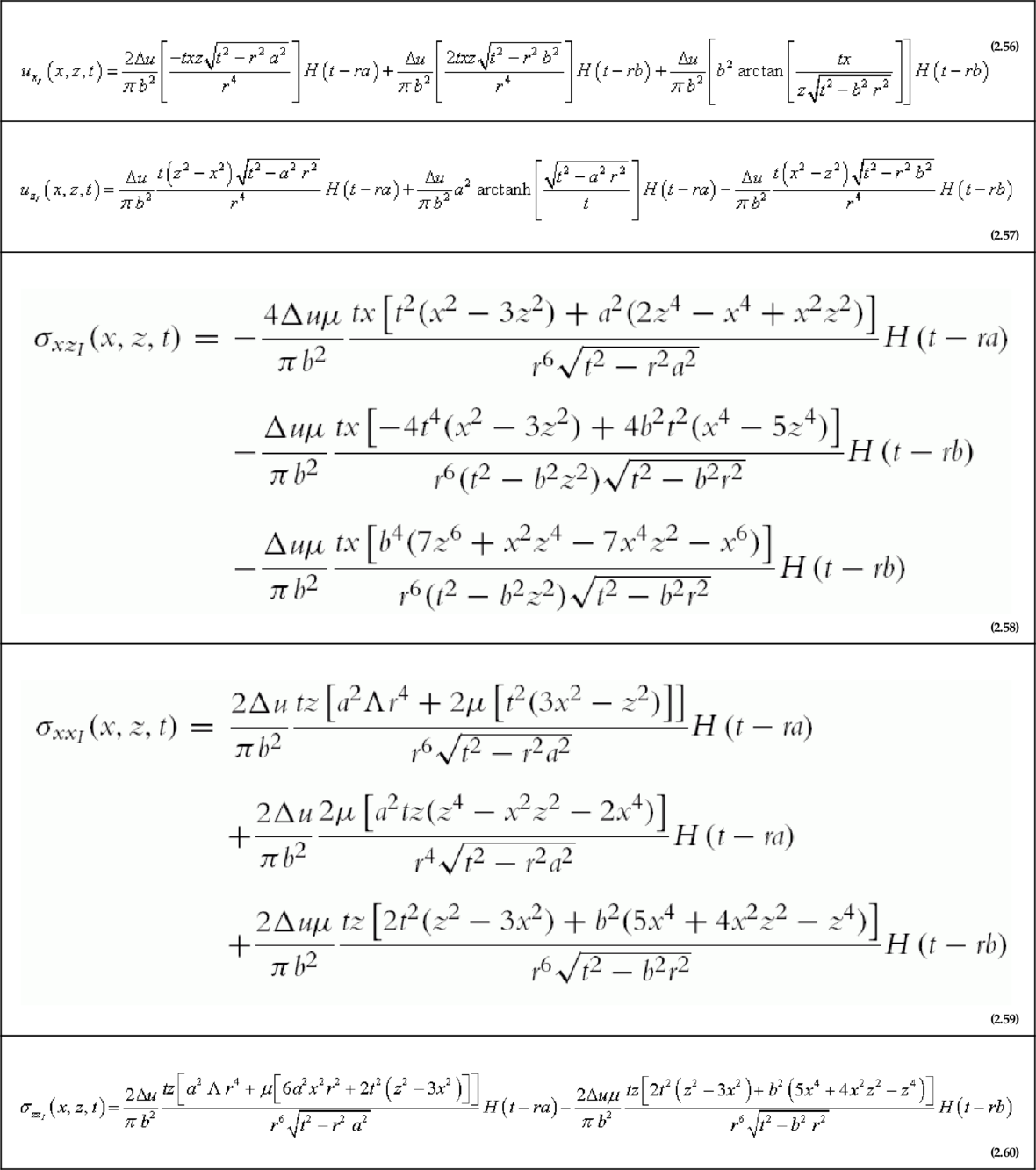
5.3 Asymptotic behavior of the injection contributions
The injection contributions in Table 2.1 describe the fields of a quiescent, nonmoving dislocations created at time t = 0. In the limit t → ∞, the solution will have propagated throughout the infinite domain. Thus, it ought to be expected that, in that limit, the solutions in Table 2.1 converge to the traditional quasi-static fields of dislocations.
This can be proven easily. Consider the limit t → ∞ of, say, the σxz component (Eq. 2.58):

And since

where B = Δu/2 is the Burgers vector, the injection contribution is seen to converge to the static one.
The same can be proven for all other components of stress and displacement.
5.4 The mobile contributions
The derivation of the mobile contributions (Markenscoff & Clifton, 1981) is analogous to that of the injected ones, but with the added complication that in this case the boundary condition,
depends on a past history function l(t) which is, in general, unknown.
The transformed governing equations are the same as before (Eqs. 2.39 and 2.40), but the integration constants must now fulfill the boundary condition above, which is first written in its equivalent form as
(where η(x) is the inverse of the past history function) and then transformed accordingly, to finally get the following transformed potentials:
The inversion of these potentials is performed using the Cagniard–de Hoop method following the same procedure as before. The resulting expressions are collected in Table 2.2.
Table 2.2
The Mobile Contributions
|
|
|
|
|
|
|
|
|
|
|
|
|
|
|
|