
7.3 The rayleigh wave speed
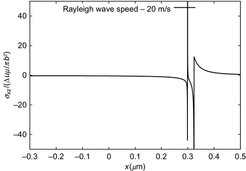
The effect of the Rayleigh wave speed over the σxz shear stress component has been briefly discussed in Section 3.3. Its true effect can be best seen by considering the σxz solution for the injected, uniformly moving dislocation found in Table 2.3.
Figure 2.32 shows the σxz stress component along the slip plane (z = 0) when the dislocation is moving with a speed 20 m/s below the Rayleigh wave speed.11 The instant in time represented is t = 0.1 ns after the injection at position x = 0, so the core has advanced to be at almost x = 0.3 μm. The discontinuity at the core is followed by the discontinuity caused by the front of the transverse wave, which delimits a narrow area of interest. Figure 2.33 shows the same dislocation, had it moved with exactly the Rayleigh wave speed. As can be seen, the singularity at the core all but disappears, as expected from Eshelby's remark that the width of the core vanishes at the Rayleigh wave speed (Eshelby, 1949b). This is followed by Fig. 2.34, which shows the same dislocation had it move 20 m/s above the Rayleigh wave speed. In this case, the sign of the field ahead of the core has reversed. This result matches that predicted by Weertman for the case of the uniformly moving preexisting dislocation (Weertman, 1961), and asymptotically by Brock for the case studied here of an injected, uniformly moving dislocation (Brock, 1982).


Hence, the solution here employed seems to display the same kind of core instability commented in Section 3.3.
The cancellation of the core's singularity at the Rayleigh wave speed can be confirmed analytically as well. Consider, for mathematical simplicity, the case of a uniformly moving preexisting dislocation. The injected case should render the same result, inasmuch as the singularity at core is of the same order (Gurrutxaga-Lerma et al., 2013).
Along the direction of the slip plane (z = 0), the shear stress component is
σxz(x,0,t)=μ4Δuπb2[−4(a2dt2x6−a2t3x5−dt4x4+t5x3)x6√t2−a2x2(d2x2−2dtx+t2)H(t−ax)−b4dx8−b4tx7−4b2dt2x6+4b2t3x5+4dt4x4−4t5x3x6√t2−b2x2(d2x2−2dtx+t2)H(t−bx)]−Dx
where D = bμ/2π(1 − ν) is the static prefactor. Recall Eq. (2.61), whereby
D=−Δuμ2(a2−b2)πb2
The dislocation's core is located at x = t/d for any given instant in time. For subsonic motion, d > b > a. Hence, Eq. (2.118) can be rewritten as
σxz=−2(a2−b2)x−4(a2dt2x6−a2t3x5−dt4x4+t5x3)x6√t2−a2x2(d2x2−2dtx+t2)−b4dx8−b4tx7−4b2dt2x6+4b2t3x5+4dt4x4−4t5x3x6√t2−b2x2(d2x2−2dtx+t2)

Expand in Taylor series about x = t/d to get
σxz=d6(x−td)(−4t(a2−d2)d6√t2−a2t2d2−t(b4−4b2d2+4d4)d8√t2−b2t2d2)+d6[−2(a2−b2)d5t−6d(4√(1−a2d2)d4t−(b2−2d2)2d8t√(1−b2d2))+4(3d2−4a2)d5t√(1−a2d2)+6b6−23b4d2+28b2d4−12d6d7(d2−b2)t√(1−b2d2)]+(x−td)[21d8t(−4(a2−d2)d6√t2−a2t2d2−b4−4b2d2+4d4d8√t2−b2t2d2)+d6t(−10(a2t4−b2t4)d4t5+2(12a4−19a2d2+6d4)d4(d2−a2)√t2(d2−a2)d2−30b8−117b6d2+166b4d4−100b2d6+24d82d6(d2−b2)2√t2(d2−b2)d2)+6d7t(−2(a2t5−b2t5)d5t6+4(3d2−4a2)d5√−t2(a2−d2)d2−−6b6+23b4d2−28b2d4+12d6d7(d2−b2)√t2(d2−b2)d2)]+O[x−td]2+higher order terms

The only term providing a singularity at x = t/d, i.e., at the position of the core of the dislocation, is the first term in Eq. (2.120). Consider its limit
limx→t/dd6(x−td)(−4(a2−d2)d6√1−a2d2−(b4−4b2d2+4d4)d8√1−b2d2)

This term diverges unless the numerator itself, a function of d, a, and b, vanishes, in which case the limit is zero because the denominator would cancel for every x, including x+ = (t/d)+ and x− = (t/d)−.
Thus, the core's singularity disappears for
d6(−4(a2−d2)d6√1−a2d2−(b4−4b2d2+4d4)d8√1−b2d2)=0

Taking the dislocation's speed d = 1/v to be variable one obtains eight different values of d for which this might happen. The only nonnegative, nontrivial real value of the solution is
d=12√3[−8·22/3a4b4−6b4κ(a2−b2)κ−3√2κ1/3(a2−b2)+4a2(b2κ+3·22/3b6)−6·22/3b8(a2−b2)κ]1/2

where
κ=3√−32a6b6+99a4b8−90a2b10+27b12+3√3b7(b2−a2)√(−64a6+107a4b2−62a2b4+11b6)

After much tedious algebra, one can check that this value is, in fact, the Rayleigh wave speed (cf. Eringen & Suhubi, 1975),
d≡1cR=1b[22/33√56ν3−123ν2+3√3√−32ν6+112ν5−165ν4+148ν3−94ν2+36ν−5+78ν−113(ν−1)−−40ν2+56ν−163·22/3(ν−1)3√56ν3−123ν2+3√3√−32ν6+112ν5−165ν4+148ν3−94ν2+36ν−5+78ν−11+83]1/2

where ν is Poisson's ratio and where the following relation has been used
ab=√1−2ν2(1−ν).
The Rayleigh wave speed in Eq. (2.125) corresponds to the solution of the Rayleigh equation (Eringen & Suhubi, 1975),
γ3−8γ2+82−ν1−νγ−81−ν=0
where γ = cR/ct.
7.4 The injected nonuniformly moving edge dislocation
The nonuniformly moving dislocation is characterized through its past history function, η(x), that returns the arrival time of the dislocation line to position x. The effect of the past history on the fields of dislocations is, to all effects, akin to the Doppler effect experienced with a moving acoustic source. It can be discerned by considering that, as it varies its speed, the dislocation will radiate outward elastic perturbations with the dynamic characteristics of a locally uniformly moving dislocation. This is reflected in the fields themselves through the appearance of undulations. These undulations which correspond to changes of velocity. For instance, Fig. 2.35A shows the σxz field of a uniformly moving edge dislocation; Fig. 2.35B shows the field of a nonuniformly moving dislocation at the same instant in time. The latter moves with a random speed varying between 0 and ct. As a result, the field is distorted with respect to the smooth fields of the uniformly moving dislocation. Figure 2.36 shows the σxx and σzz components of a nonuniformly moving dislocation with speed between Mt = 0 and Mt = 0.62; again, the fields are not smooth as a result of terms corresponding to different speeds having been radiated by the core at past time steps.
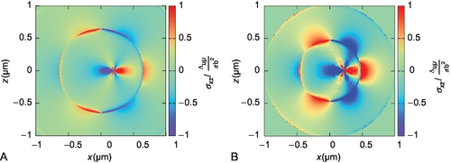
 0.5 ≡ 1618 m/s. (A) Uniform speed. (B) Random speed per time step. Image courtesy of Gurrutxaga-Lerma et al. (2013).
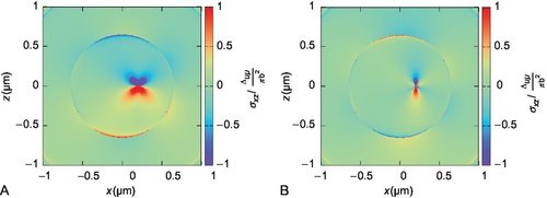
The nonuniformly moving dislocation's fields highlight the importance of the past history: if it is neglected in favor of uniformly moving dislocations, the fields become smooth but falsified.
7.5 The annihilation of dislocations
The annihilation of dislocations is a well-known phenomenon (Hirth & Lothe, 1991). It occurs when two unlike-signed dislocations get close enough to one another that their mutually attractive forces overcome the external driving forces, making them attract each other. Once they are within a Burgers vector distance of one another, their respective Burgers vectors cancel each other and, therefore, the dislocations annihilate one another.
In quasi-static discrete dislocation dynamic methods including DDP, annihilations are instantaneous. However, in D3P, and as result of the time dependency of the elastodynamic fields of dislocations, annihilations cannot be instantaneous any longer. This is because any information about the annihilation having taken place has to travel to the rest of the medium at the speeds of sound.
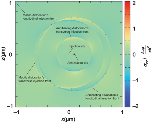
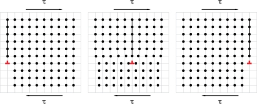
This can be better understood by consider the following situation: an injected, uniformly moving dislocation reaches a given position, where an unlike signed static dislocation is injected. Figure 2.37 shows the resulting annihilation process. The fields radiated by the newly injected dislocation cancel those of the previous one, which will have been stopped and begun to radiate from the annihilation position. However, the injected dislocation's fields cannot cancel those existing before it was injected, and their longitudinal components cannot cancel the transverse components of the moving dislocation. Hence, cancellation only occurs identically inside the transverse injection front of the injected dislocation (vid. Fig. 2.37), and there are remanent fields that a dislocation dynamics method must account for throughout the simulation.
8 Methodological rules
Sections 5–7 deal with the description, implementation, and implications of the elastodynamic fields of an injected, nonuniformly moving dislocation and associated problems. However, as stated in Section 2, any dislocation dynamics method requires the definition of additional methodological or constitutive rules for its closure.
D3P arises as an extension of DDP and, indeed, many of the constitutive rules used in this method will closely resemble those of DDP (vid. Van der Giessen & Needleman, 1995). However, the causality and retardation effects introduced through the elastodynamic fields of dislocations produce a fundamental change of paradigm with respect to DDP and, in general, with respect to all dislocation dynamics methods.
In this section, the main methodological aspects of D3P are presented, and the differences with DDP are highlighted throughout. Unsurprisingly, the main differences between DDP and D3P are caused by the time dependency of the elastic fields. This occurs in two ways. On one hand, the dynamic fields of dislocations will affect dislocation interactions and reactions. For instance, as explained in Section 7.5, dislocation annihilations are not instantaneous in D3P; equally, all interactions are based on a retardation principle, albeit contained in the formulation of the fields of the dislocations themselves, so it requires no constitutive treatment.
On the other hand, the formulation of the dynamic fields of dislocations presented above is associated with specific boundary conditions, the characteristics of which introduce significant changes to certain constitutive rules, especially those related to the mobility laws of dislocations and the generation rules. As highlighted in Section 4, D3P is particularly necessary when the boundary conditions are such that the representative speed of the system is a significant fraction of the transverse speed of sound. For instance, in Section 4, the need for a dynamic formulation was justified as necessary to simulate the plastic relaxation processes under shock loading. Shock loading might not be the only situation where D3P is needed,12 but it is representative of them all: a process where the response of the material is in the same timescale as the propagation of both the boundary conditions and the fields of the dislocations.
Here, the methodological modifications in D3P are aimed at examining how each of the physical processes they represent is modified in a fast-paced, high load situation. In this section, particular focus is given to how the mobility laws of dislocations and the generation rules of dislocations change under shock loading. A comprehensive treatment able to cover the whole spectrum of timescales is provided. Moreover, the results presented here can be extended to any other situation where dislocations are expected to move at a significant fraction of the speed of sound.
Thus, this section is structured as follows: first, the integration scheme based on the linear superposition principle is presented; then, the mobility laws are assessed, followed by the operation of Frank–Read sources and homogeneous nucleation. Finally, the general slip plane geometries are presented, and the relevance of the elastic constants is briefly described.
8.1 The integration scheme
The expressions of the elastic fields of dynamic dislocations presented in Tables 2.1–2.3 are valid only for an infinite domain. These comprise the application of external boundary conditions in finite-sized domains (for instance, an impact load over an finite plate), so the direct application of the formulas given in those tables is not possible.
As in DDP, the infinite domain fields are used for finite-sized problems through the linear superposition principle. As explained in Section 2.1, the application of the superposition principle to dislocation dynamics was first proposed by Lubarda et al. (1993) and used thereafter by researchers following Van der Giessen and Needleman's (1995) approach to DDP. Its essence is summarized in Fig. 2.38.
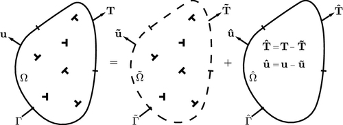
Little modification to the procedure illustrated in Fig. 2.38 is required in a fully dynamic formulation such as D3P because the linear superposition principle remains true for each instant in time. Let Ω be the boundary value problem's domain, and let σ (x, t), u(x, t) be the stress and displacement fields therein. By virtue of the linear superposition principle, these can be conceived as the sum of two fields: σ=˜σ+ˆσ![]() and u=˜u+ˆu
and u=˜u+ˆu![]() , where ˜σ
, where ˜σ![]() and ˜u
and ˜u![]() are the stress and displacement fields of the dislocations in the infinite domain ˜Ω
are the stress and displacement fields of the dislocations in the infinite domain ˜Ω![]() and where ˆσ
and where ˆσ![]() and ˆu
and ˆu![]() are the stress and displacement fields of a finite-size media ˆΩ
are the stress and displacement fields of a finite-size media ˆΩ![]() directly mapping onto Ω, where the boundary conditions are applied.
directly mapping onto Ω, where the boundary conditions are applied.
Let Γ be the boundary of Ω. In the infinite domain, Γ is mapped onto ˜Γ![]() ; over that surface, there is a traction ˜T
; over that surface, there is a traction ˜T![]() and a displacement ˜u
and a displacement ˜u![]() . If the superposition of ˆΩ
. If the superposition of ˆΩ![]() and ˜Ω
and ˜Ω![]() is to result in Ω, the resulting Γ surface must be traction and displacement free except for where the boundary conditions are applied. This can only be achieved if the ˆΓ
is to result in Ω, the resulting Γ surface must be traction and displacement free except for where the boundary conditions are applied. This can only be achieved if the ˆΓ![]() surface has, for every instant in time, the negative of ˜T
surface has, for every instant in time, the negative of ˜T![]() and ˜u
and ˜u![]() applied over it. Thus, if ˆΩ
applied over it. Thus, if ˆΩ![]() experiences both the boundary conditions and the reversed tractions and displacements, the finite-size problem can be tackled as usual, no image fields being necessary.
experiences both the boundary conditions and the reversed tractions and displacements, the finite-size problem can be tackled as usual, no image fields being necessary.
In turn, the ˜Ω![]() elastic field can be obtained through linear superposition of each dislocation's infinite domain fields:
elastic field can be obtained through linear superposition of each dislocation's infinite domain fields:
˜u=∑i˜ui,˜σ=∑i˜σi,˜e=∑i˜ei
where ˜ui![]() , ˜σi
, ˜σi![]() , and ˜ei
, and ˜ei![]() denote dislocation i's displacement, stress, and strain fields. Further details can be found in Van der Giessen and Needleman (1995).
denote dislocation i's displacement, stress, and strain fields. Further details can be found in Van der Giessen and Needleman (1995).
8.2 Integration scheme
In general, the ˆΩ![]() domain can be solved using the finite element method or any other elastodynamic numerical scheme; the ˜Ω
domain can be solved using the finite element method or any other elastodynamic numerical scheme; the ˜Ω![]() domain is provided by the formulation presented here. This leads to the total elastic fields over the finite domain. However, it does not describe the evolution over time of the dislocation structure: a mobility law is required.
domain is provided by the formulation presented here. This leads to the total elastic fields over the finite domain. However, it does not describe the evolution over time of the dislocation structure: a mobility law is required.
D3P can achieve a full description of the evolution and interaction of dislocation structures in 2D by adopting an Euler-forward scheme as follows:
1. At time t, calculate ˜T![]() and ˜u
and ˜u![]() in ˜Ω
in ˜Ω![]() .
.
2. Applying −˜T![]() and −˜u
and −˜u![]() over ˆΓ
over ˆΓ![]() in ˆΩ
in ˆΩ![]() , advance the dynamic solution, a time step.
, advance the dynamic solution, a time step.
3. Obtain the global stress fields as σ=ˆσ+˜σ=ˆσ+∑i˜σi![]() at each current dislocation position and on sources and obstacles. Note that in the case of a dislocation, self-stress is omitted from the sum.
at each current dislocation position and on sources and obstacles. Note that in the case of a dislocation, self-stress is omitted from the sum.
4. Calculate the corresponding Peach–Koehler forces acting on dislocations using σ.
5. Resolve the interaction, creation, and motion of dislocations using the constitutive rules, updating their positions according to the mobility law by a time step dt.
6. Repeat from 1.
8.3 Slip systems
Dislocation generation and motion occurs only in specific systems of slip that reflect the directions in which dislocation motion is most favorable. Slip tends to occur in close-packed planes of atoms. In FCC materials, slip occurs principally in the close-packed {1 1 1} family of atomic planes (Hirth & Lothe, 1991). Slip planes are not so well defined in BCC materials (Hirth & Lothe, 1991; Hull & Bacon, 2011; Kubin, 2013), but slip tends to occur in the 〈1 1 1〉 direction, which is contained by the {1 1 0}, {1 1 2}, and {1 2 3} planes (Hull & Bacon, 2011).
In D3P, slip systems are selected in the same way as in DDP (vid. Van der Giessen & Needleman, 1995). Thus, in D3P the slip systems in the 2D plane are straight lines with specific orientations relative to the axes of the 2D plane, which are usually defined along the [0 1 0] and [1 0 1] directions. The slip planes have to be such that they fulfill the plane strain requirement of DDP and D3P (Van der Giessen & Needleman, 1995) and, at the same time, they must resemble the crystallography of the material.
In cubic crystals, the slip systems that fulfill the plane strain requirement were derived by Rice (1987), who provided a detailed analysis and justification. These can be found in Figs. 2.39 and 2.40.


FCC crystals. In FCC crystals, slip occurs in {1 1 1} planes in 〈1 1 0〉 directions (Hirth & Lothe, 1991; Hull & Bacon, 2011). This amounts to 12 different slip systems. In the 2D plane, they are reduced to three different directions (Rice, 1987), located at 54.7°, 70.5°, and 54.7° of one another (Rice, 1987). See Fig. 2.39.
BCC crystals. As said above, in BCC crystals, there is no truly close-packed plane (Hull & Bacon, 2011); slip is generally expected to occur in {1 2 1} and {1 0 1} planes (Ito & Vitek, 2001; Vitek, 1992), with the slip direction being 〈1 1 0〉. In the 2D plane, they are reduced to three different directions, located at 70.5°, 54.7°, and 54.7° of one another. Thus, the BCC slip systems are homologous to the FCC systems, with a 90° rotation (Rice, 1987). See Fig. 2.40.
The specific slip systems selected in DDP and D3P are necessary to ensure the plane strain requirement is satisfied. For the simulation of shock loading in D3P, this is particularly convenient. As shown in Fig. 2.41, in many shock-loading experiments the shock front is assumed to propagate in the [1 0 0] direction (Meyers et al., 2003, 2009). The large uniaxial loads, the crystallographic orientations, and the higher energy penalty associated with generating edge components rather than screw components make it more likely that the dislocation loops will expand in a manner similar to that depicted in Fig. 2.41, with the screw components lying on 〈1 1 1〉 directions and edge components on the 〈1 1 0〉 directions—perpendicular to the (0 1 0) plane. Experimental evidence also suggests a residual population of dislocations made up principally of screw components (Meyers et al., 2009). All this suggests that edge components are the principal agents of plasticity in typical shock loading experiments; hence, the dislocations are under plane strain conditions.

Finally, one must bear in mind that the shock load and, consequently, the large compression of the crystalline lattice will tend to produce a rotation in the crystallographic planes (Meyers, 1994; Shehadeh et al., 2005). D3P does not account for that rotation in the slip systems. Furthermore, as a result of the compression of the lattice, one should observe a change in the values of the elastic constants. This change is not expected to be exceedingly large, especially for the speeds of sound because the elastic constants will increase in similar proportion to the density. Accounting for load-induced changes in the elastic constants in a continuum model is challenging. Furthermore, dislocation theory would need to be adapted13 as well, because the fields of dislocations, either static or dynamic, require the homogeneity of the continuum medium.
8.4 Mobility laws
The mobility law of a dislocation segment relates one or more of the segment's kinematic variables (its velocity, acceleration,…) to any of the external stimuli that may be acting upon the dislocation segment. The external stimuli are usually elastic fields, originating either from the boundary conditions or from other dislocations. Mobility laws are necessary to describe the motion of dislocations in the continuum framework because elasticity only provides a geometric description of the long-range fields of the dislocations, not how dislocations respond to applied stress (Mura, 1963).
The principal requirement of mobility laws is that they ought to faithfully describe the physics of the motion of dislocations. Two remarks must be made in this respect: that dislocations tend to move so as to minimize the elastic energy of the medium (Hirth, 1996; Hirth & Lothe, 1991); and that in their motion, dislocations lose energy through dissipative mechanisms (Hirth & Lothe, 1991; Hull & Bacon, 2011; Nabarro, 1967).
Irrespective of the specific governing mechanisms, mobility laws employed in discrete dislocation dynamics methods must reflect these two criteria. The requirement that dislocations move to minimize the elastic energy of the system can be thought of as a driving mechanism that is balanced by the fact that, in their motion, dislocations radiate energy. Thus, most mobility laws in dislocation dynamics are usually expressed as energy or force balances between variables which respect these two criteria.
Typically, the influence of any external elastic field over a dislocation segment is expressed through the so-called Peach–Koehler force (vid. Peach & Koehler, 1950), given by
fn=εnjmσijbiξm
where a repeated index denotes summation, σij is the tensor of external stresses, ξm is the direction of the dislocation segment, bi the Burgers vector, and εnjm the Levi-Civita tensor.
The Peach–Koehler force is “a virtual thermodynamic force and must not be confused with a mechanical one” (Hirth, 1996). This is of great importance. A virtual thermodynamic force is derived from an energy field, as its negative gradient
fi=−∂g∂Xi

where g denotes the Gibbs potential, in this case corresponding to the elastic energy external to the dislocation, and Xi is a reaction coordinate, in this case the displacement of a local dislocation segment. From Eq. (2.129), it could be said that the Peach–Koehler force is a dynamic14 equivalent to an energy; specifically, it is the gradient of the elastic energy of the system, pointing in the direction of maximum change in the external elastic energy field. As said above, the dislocation will move in such a way as to minimize the elastic free energy of the system; the Peach–Koehler force becomes the favored way of defining mobility laws because, it follows, its direction is that of the motion (Hirth, 1996; Kubin, 2013) and, as a gradient, it serves as a measure of the changes in the elastic energy of the system. Following the remarks made above that the dislocation's motion itself is dissipative, equating the Peach–Koehler force to some dissipative force (energy output) in a mobility law simply expresses an energy balance over the dislocation; the specific form of this balance usually relates one or several kinematic variables of the dislocation, therefore defining its motion.
8.4.1 The regimes of motion of a dislocation
The definition of the dissipative force requires a description of the physics of dislocation motion in some depth. First, it is necessary to recognize that dislocation motion is composed principally of glide and climb. Glide refers to the conservative motion of the dislocation within its own slip plane, and climb to the nonconservative motion of the dislocation perpendicular to the slip plane (Hirth & Lothe, 1991). Climb is a diffusion-assisted process (Argon, 2008), usually deemed too slow to be present in any high strain rate situation; hence, it will be omitted from further discussion. The reader is referred to Hirth and Lothe (1991) and Balluffi, Allen, and Carter (2005) for further discussions on dislocation climb. Glide, in turn, only requires mechanical stresses to occur (Hirth & Lothe, 1991); the process can be best understood in Fig. 2.42 for an edge dislocation in a simple cubic lattice.
As can be seen in Fig. 2.42, glide involves breaking and rebuilding interatomic bonds. At the core of the dislocation, it is an inherently atomistic process. It is conceivable that as the dislocation's core advances, breaking and rebuilding bonds acts as a dissipative process (Nabarro, 1967), where multiple lattice vibrational modes are excited, resulting in a net radiation of energy outward from the core. Relating this energy loss to the applied external fields that drive the dislocation motion—i.e., the Peach–Koehler force over the dislocation—ought to, in principle, allow the definition of a mobility law. However, the exact details of these processes are far from simple.
It is commonly observed, both experimentally (Johnston & Gilman, 1959; Nix & Menezes, 1971) and in MD simulations (Bitzek & Gumbsch, 2004, 2005; Koizumi et al., 2002; Olmsted et al., 2005; Tsuzuki et al., 2008), that dislocation glide is severely overdamped (Gilman, 1969) and directly proportional to the dislocation's velocity in a manner similar to a viscous drag force in fluid motion (Gilman, 1969; Hirth, 1996; Hirth & Lothe, 1991; Hull & Bacon, 2011). This was in fact first established by Leibfried (1950), who proposed the drag force of the form
fdrag=d·vglide
that can be found in most text books on the subject (vid. Argon, 2008; Bulatov & Cai, 2006; Hirth & Lothe, 1991; Hull & Bacon, 2011; Kubin, 2013; Nabarro, 1967; Reed-Hill & Abbaschian, 1994).
The most ubiquitous of mobility laws found in dislocation dynamics, both DDP and 3D DD, equates this viscous drag force fdrag (Eq. 2.130) to the glissile component of the Peach–Koehler force because, as has been said above, the dislocation moves so as to minimize the elastic energy of the system following the Peach–Koehler force, and that the energy reduction is dissipated by the dislocation in its motion through this viscous drag process. For the motion of straight edge dislocations of interest to D3P, the glissile component of the Peach–Koehler force is15 merely fglide = τ · B with τ the resolved shear stress over the slip plane and B the magnitude of the Burgers vector, so the balance renders a mobility law of the form
vglide=τBd
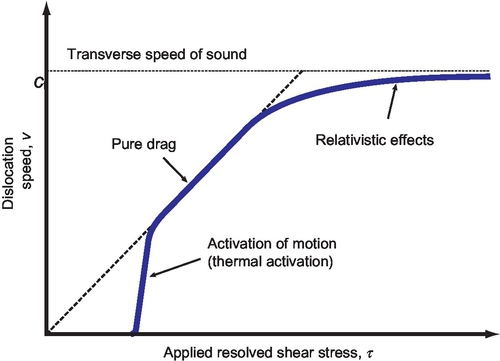
However, the validity of the mobility law defined in Eq. (2.131) is far from universal and depends on, among other things, the levels of applied stress. Figure 2.43 summarizes the regimes of motion of a dislocation. As can be appreciated there, there are at least three distinct regimes for the motion of a dislocation, each of which leads to different mobility laws.
8.4.2 Drag-controlled regime
The regime of dislocation velocities for which the viscous drag law (Eq. (2.131)) is applicable is called the “drag-controlled regime.” In the drag-controlled regime, dislocation motion is dominated primarily by phonon drag, i.e., by the interaction between the dislocation and the thermal vibrations in the lattice. Phonon drag is mainly mediated by phonon scattering (Gilman, 1969; Granato, 1973; Hirth & Lothe, 1991; Hull & Bacon, 2011; Nabarro, 1967), which seems to involve mainly two processes (vid. Granato, 1973). On one hand, the dislocation itself will strain the lattice around its core, thereby breaking its symmetry. As the dislocation moves through the lattice, this strained region will be met by the incoming thermal phonons from elsewhere in the lattice that will be refracted as a result. On the other hand, phonons may be absorbed by the dislocation itself, triggering vibrations of its core that, again, result in new phonons radiated outward. The result is that dislocations in the drag-controlled regime move with linear viscous drag laws such as that shown in Eq. (2.131).
8.4.3 Thermal activation regime
The lower limit of the drag-controlled regime marks the onset of dislocation motion. In this regime, dislocation motion occurs in the presence of low applied stresses, so low that the motion of dislocations is dominated by those mechanisms that offer direct resistance to the motion. A dislocation can encounter resistance to its motion from two kinds of sources: the crystalline lattice itself and obstacles. The intrinsic resistance of the lattice to the motion of dislocations refers to the energy cost associated with breaking and rebuilding interatomic bonds as the dislocation moves; this effectively manifests itself in the periodic16 Peierls barrier (Granato, 1973; Regazzoni et al., 1987). Obstacles refer to lattice imperfections that may include impurities, interstitials and vacancies, other dislocations, etc. These obstacles interact with the dislocation hindering its motion; unlike the Peierls barrier however, obstacles do not offer a periodic resistance. In either case, both the intrinsic lattice resistance and obstacles can be thought of as barriers of stress that the dislocation must overcome in order to move. Focusing on the intrinsic lattice resistance alone, the magnitude of the barrier, usually called the Peierls stress or intrinsic lattice resistance, sets up a mechanical threshold of applied stress below which dislocation motion is not, in principle, possible. This threshold can still be overcome, however, through thermally assisted processes (vid. Argon, 2008; Kocks, Argon, & Ashby, 1975; Regazzoni et al., 1987), whereby thermal energy helps the dislocation overcome the barrier. For this reason, the lower regime is sometimes called the “thermal activation regime” or “activation of motion regime.”
The thermal activation regime is often associated not only with the onset of dislocation motion, but of plasticity as a whole. This is true in a sense, but it may suggest that before moving into the drag-controlled regime, dislocations must overcome the thermal activation regime—i.e., that the onset of all dislocation motion is always thermally activated. This might be true at low strain rates and low levels of stress, and in those situations, it would be consistent with the empirical observation that the yield point tends to decrease with increasing temperature. However, as has been pointed out in the introduction, the yield point of most metals experiences a sudden upturn (vid. 2.2) that has been associated with a fundamental change in the dislocation's own motion regime, going from thermally activated to drag controlled Regazzoni et al. (1987). Undoubtedly, a dislocation in a material shock loaded to 20 GPa with a strain rate of 1010 s−1 will hardly have time, if any, to go through the thermally activated regime. Hence, there are situations that are particularly relevant to D3P, where the thermally activated regime is not relevant.
8.4.4 Relativistic regime
The upper limit of the drag-controlled regime is usually a velocity of the order of tens or a few hundreds of meters per second. Surpassing this limit is unusual in most plasticity applications. In fact, DDP simulations typically cap the speed of dislocations at ≈ 20 m/s (cf. Cleveringa, Van der Giessen, & Needleman, 1997). The regime of motion beyond the drag-controlled regime is often called the “relativistic regime.” This is because the speeds reached in this regime are usually a significant fraction of the transverse speed of sound, and therefore, the relativistic effects discussed in Section 3.2 are expected to be present. Typically, in this regime the speed of dislocations saturates toward the transverse speed of sound (Gilman, 1969; Johnston & Gilman, 1959; Marian & Caro, 2006; Meyers, 1994; Olmsted et al., 2005).
As shown in Section 3.1, in the “relativistic regime” the elastic energy of dislocations tends to increase with the speed of dislocations, diverging at the transverse speed of sound. This is of great significance, as it shows that even the mobility laws commonly employed in dislocation dynamics (such as Eq. (2.131)) are in fact quasi-static. The reason is simple: as it moves, the self-energy of the dislocation itself must change. This change is negligible for the low speeds encountered in the drag-controlled regime, but it becomes significant at higher speeds—i.e., in the relativistic regime. If the speed of the dislocation is going to increase, the elastic energy of the dislocation will increase; the energy input due to the external fields (the Peach–Koehler force), that in quasi-static mobility laws only had to balance out the drag dissipation, will now also have to be spent on increasing the dislocation's elastic energy as well. To wit, quasi-static mobility laws do not account for changes in the elastic energy of the dislocation itself, which is expected to vary in dynamic cases.
Thus, the dynamic mobility law has to be modified to include one way or another the contribution of the dislocation's self-energy. This leads to several questions:
• Is the Peach–Koehler force itself, derived for time-independent fields, affected in dynamic situations?
• How does the increase of the dislocation's elastic self-energy affect the mobility law?
• Is the viscous drag force the main dissipative mechanism at play in the relativistic regime?
These questions will be addressed in the following sections.
8.4.5 The exactitude of the peach–koehler force
As originally derived by Peach and Koehler (1950), the Peach–Koehler force given in Eq. (2.129) accounts for variations in the external elastostatic energy. However, D3P uses a fully elastodynamic formulation, so one must establish its exactitude when time is an explicit elastic field variable. The considerations presented here were pioneered by Lothe (1961) and Stroh (1962), and rigorously formalized by Mura (1982). It is shown that the Peach–Koehler force as given by Eq. (2.129) is to be exact in a dynamic framework.
In order to show this, consider a moving dislocation loop in an infinite domain D. The associated Lagrangian functional shall be:
L=∫D(12ρ˙ui˙ui−12σijεij)dD

where T=12∫Dρ˙ui˙uidD is the kinetic energy density and V=12∫DσijεijdD
![]() the potential (elastic) energy density. Thus, L=T−V
the potential (elastic) energy density. Thus, L=T−V![]() is the Lagrangian density. Notice that the Lagrangian proper would be
is the Lagrangian density. Notice that the Lagrangian proper would be
L=∫t1t0Ldt
Elastodynamics require that σijεij = σijui,j, so
∫t1t0Ldt=∫t1t0dt∫D(12ρ˙ui˙ui−12σijui,j)dD

This expression is defined everywhere in the domain except on the slip surface S, where a discontinuity arises. The boundary of S is the dislocation line L, which shall be assumed to move with a velocity field ˙ξi![]() , so that ξi is taken to be the displacement of the line. Over the dislocation line, the dislocation's discontinuity can be expressed through the following boundary condition:
, so that ξi is taken to be the displacement of the line. Over the dislocation line, the dislocation's discontinuity can be expressed through the following boundary condition:
u+i(x,t)−u−i(x,t)=bi
The conditions that ξ must fulfill for the Lagrangian functional L to be minimized must be found. For that, in a dynamic situation, a virtual displacement δξ over the dislocation line is imagined that produces a change δS over the slipped region. In order to find out how this change is bounded by the principle of least action, the variation of the functional is considered:
δ{∫t1t0Ldt}=∫t1t0dt∫D(ρ˙uiδ˙ui−σijδui,j)dD
Operating:
δ∫t1t0Ldt=∫t1t0dt∫D(ρ˙ui∂∂t(δui)−σij∂∂xj(δui))dD

Applying Gauss's theorem, one must bear in mind that D is not simply connected, so that S + δS must be excluded by defining an infinitely closed enveloping surface made of S+ + δS+ and S− + δS−. Excluding that surface, Gauss's theorem leads to
∫Dσij∂∂xj(δui)dD=∫S+δSσijnj[δui]dS−∫Dσij,jδuidD=∫δSσijnjbiδS−∫Dσij,jδuidD

where the apparent sign reversal is caused by the need of excluding the inner side of S + δS rather than the outer one. Here [ui] is the difference of ui being evaluated at the upper and lower surfaces of the slip plane (the integral is divided into ∫S++S−+∫δS++∫δS−≡∫S+δS . Hence, [ui] = bi on S. After the virtual displacement δξi, its variation [δui] = δ[ui] is therefore zero on S and bi on the new virtual slipped region δS.
The δS is the variation of the slipped region S, which arises from a virtual displacement δξi and thus must fulfill the same condition as in the static case:
njδS=εjlhδξlνhdl
Furthermore, it is found that
∫t1t0ρ˙ui∂∂t(δui)dtdD=−∫δSρ˙uibi˙ξjnjδS−∫t1t0ρ¨uiδuidtdD

Grouping everything into the functional
δ∫t1t0Ldt=−∫t1t0dt∮L(ρ˙ui˙ξj+σij)biεjlhδξlνhdl

The term ρ˙ui˙ξjbiεjlhνh![]() is called the Lorentz force for its analogy with the electrodynamic Lorentz force. A detailed analysis of the Lorentz force was presented by Lund (1998). It is of great mathematical interest, but of little physical significance because, as its electrodynamic counterpart, it does no work. Indeed, ˙ξjdt=δξj
is called the Lorentz force for its analogy with the electrodynamic Lorentz force. A detailed analysis of the Lorentz force was presented by Lund (1998). It is of great mathematical interest, but of little physical significance because, as its electrodynamic counterpart, it does no work. Indeed, ˙ξjdt=δξj![]() , which in the Lorentz force term leads to having εjhlδξjδξl = 0 necessarily. Hence, as stated by Lund (1998): “the additional “Lorentzian” force that is (…) orthogonal to the dislocation velocity, [so] it does not do any work”; in order to establish its relevance, it would be necessary to explain what the Lorentz force would physically entail. Otherwise, the variation of the functional leads to
, which in the Lorentz force term leads to having εjhlδξjδξl = 0 necessarily. Hence, as stated by Lund (1998): “the additional “Lorentzian” force that is (…) orthogonal to the dislocation velocity, [so] it does not do any work”; in order to establish its relevance, it would be necessary to explain what the Lorentz force would physically entail. Otherwise, the variation of the functional leads to
δ∫t1t0Ldt=−∫t1t0dt∮Lσijbiεjlhδξlνhdl
It could be imagined that the dislocation is subjected to a force rather than to an external stress field. Looking at the expression above, this would lead, as in the static case, to the Peach–Koehler force: the dynamic effects account for in ˙ξi![]() via the Lorentz force do not contribute to the energy balance and, therefore, the Peach–Koehler force is valid in the dynamic case.
via the Lorentz force do not contribute to the energy balance and, therefore, the Peach–Koehler force is valid in the dynamic case.
Indeed,
δ∫t1t0Ldt=−∫t1t0dt∮Lflδξldl

would be the variation in the action due to a force fl, and by comparing with the expression above
fl=εjlhσijbiνh
as in the static case, q.e.d.
8.4.6 Inertial forces
The Peach–Koehler force concerns forces over dislocations; these forces exert work during the dislocation's motion. In turn, the elastic energy of moving dislocations increases as the velocity of dislocations increases (and vice versa). Thus, in a dynamic situation part of the energy input due to the Peach–Koehler force must be spent in increasing the dislocation's self-energy. This is usually called the “inertial” effect (Hirth, Zbib, & Lothe, 1998), because as with inertia, it opposes changes in the motion of a dislocation, and because the effect can be translated into an equivalent thermodynamic force of the form of a Newtonian inertial force, directly proportional to a dislocation “mass” and the dislocation's acceleration.
The inertial force can be estimated with the following considerations, similar to those found in Hirth et al. (1998). Consider a straight edge dislocation in an infinite plane. Let v be its velocity. The Hamiltonian of the system can be written as
H=T+V
where T is the kinetic energy of the dislocation, and V the potential (elastic) energy of the dislocation.
Of interest here is to derive from the Hamiltonian an equivalent configurational force. Consider a straight edge dislocation moving uniformly with speed v along the X-axis. Let x be the canonical coordinate along that very same direction. Define p to be the linear quasi-momentum of the dislocation. Then Hamilton's equations require that
dpdt=−∂H∂x

dxdt=∂H∂p

It is noticed that the force can be defined as
F=dpdt

Furthermore, dxdt=ν where v is the dislocation's speed. In the context of moving dislocations, this force will be a configurational or self-force.
For the uniformly preexisting edge dislocation, Weertman (1981) found the expressions of the kinetic and elastic energy of a uniformly moving straight edge dislocation, given by:
T=E021M2t[4γl+4γl+γ3t−5γt−5γt+1γ3t]
V=E021M2t[12γl+4γl−γ3t−9γt−7γt+1γ3t]

where γt=√1−M2t![]() , γl=√1−M2l
, γl=√1−M2l![]() , and E0=μB24πln(Rrc)
, and E0=μB24πln(Rrc)![]() is the dislocation's energy at rest, where R and rc are the inner and outer cutoffs of the core.
is the dislocation's energy at rest, where R and rc are the inner and outer cutoffs of the core.
It follows that, in this framework, T = T(v) and V = V(v), so accordingly H = H(v) alone. Hence,
∂H∂x=0
so from Eq. (2.146) it is found that the quasi-momentum is invariant in time dpdt=0 , and from Eq. (2.151) that the Hamiltonian (here, the total energy) of the system is symmetric with respect to any given displacement. To wit, as in the quasi-static case, the uniformly moving dislocation does not radiate energy, and the fields are always the same as it moves.
However, ignore this last point for the moment. Invoking the chain rule
v=dxdt=∂H∂p=∂H∂tdtdp=1F∂H∂t
so that the force
F=1v∂H∂t=1v∂H∂v∂v∂t

Equation (2.153) takes the form of an inertial force provided that the effective “mass” m of the dislocation is defined as
m={∀{F,v,t}∃m|F=dvdt}

From Eq. (2.153), it is found that
m=1v∂H∂v

Since H = T + V, substituting Eqs. (2.149) and (2.150) in Eq. (2.155), one obtains that the uniformly moving edge dislocation's effective mass:
m=E021c2tM4t[−8γl−20γl+4γ3l+7γt+25γt−11γ3t+3γ5t]

This expression is entirely comparable to that obtained by Hirth et al. (1998), who used the Lagrangian formalism instead.
Thus, there seems to exist a force associated with the elastic and kinetic fields of dislocations, given in the form of an inertia force:
F=m∂v∂t

This force exists solely because the dislocation has a velocity. As with the Peach–Koehler force, it is important to recognize that it is not a mechanical force, but a thermodynamic virtual force.
At this point, it is natural to be perplexed by the inherent paradox that an uniformly moving dislocation—i.e., a dislocation where v = constant—could have an inertia. From Eq. (2.157), it seems obvious that it does not, for ∂ν∂t=0 when the dislocation is moving uniformly. Using a far more sophisticated approach, Ni and Markenscoff (2008) reached the same conclusion for a uniformly moving dislocation.
This casts doubt on the dislocation's effective mass as defined by Eq. (2.156). As mentioned above, from Eqs. (2.146), (2.149), and (2.150), it follows that for a uniformly moving dislocation, the quasi-momentum is invariant in time. In Eq. (2.152), however, one must assume that dtdp![]() exists. However, if p is not a function of t, then its inverse function t = t(p) does not exist,17 and hence dtdp
exists. However, if p is not a function of t, then its inverse function t = t(p) does not exist,17 and hence dtdp![]() is illegitimate.18 It follows that in that case v cannot be written as
is illegitimate.18 It follows that in that case v cannot be written as
v=1F∂H∂t
which suggests that the effective mass should not be defined in the case of a uniformly moving dislocation. It is important to note that the derivation above is essentially correct apart from the above mentioned contradiction.
This raise the question, what could the effective mass obtained in Eq. (2.156) possibly mean? First of all, it must be pointed out that, mathematically, it remains legitimate to define a function m such that it fulfills Eq. (2.155) even if, as said, there is no inertial force as such. This is because H = H(v) and therefore ∂H∂ν![]() exists. Consider Eq. (2.155), from which the effective mass has been derived. There, the mass is expressed as a measure of the change in the total energy (the Hamiltonian) of the dislocation as the dislocation's speed is varied. In the case of the uniformly moving dislocation, the dislocation cannot change its speed by construction; however, one can compare two dislocations moving at different speeds. Their associated energies are different; hence, it is possible to study how the energy varies for dislocations moving uniformly with different speeds. Then m as defined in Eq. (2.156) is a measure of that radiation.
exists. Consider Eq. (2.155), from which the effective mass has been derived. There, the mass is expressed as a measure of the change in the total energy (the Hamiltonian) of the dislocation as the dislocation's speed is varied. In the case of the uniformly moving dislocation, the dislocation cannot change its speed by construction; however, one can compare two dislocations moving at different speeds. Their associated energies are different; hence, it is possible to study how the energy varies for dislocations moving uniformly with different speeds. Then m as defined in Eq. (2.156) is a measure of that radiation.
It can then be argued that, as a rough approximation, the inertial force defined through Eq. (2.156) is a measure of the additional energy that is required for the dislocation to increase its steady-state speed v. This would entail that the dislocation transitions from a uniform speed to another, different, uniform speed. This clearly goes against the hypothesis employed here. However, since the dynamic fields of dislocations reach their steady-state values in a short amount of time, it can be argued that it serves as a measure of the energy required to accelerate the dislocation, and hence as an approximation to the true inertia.
A complete treatment of the inertia of a dislocation requires the expressions of T and V for the nonuniform motion of a dislocation. Unfortunately, as in the derivation of the elastodynamic fields of dislocations provided in Section 5, obtaining the inertial force of a nonuniformly moving dislocation is far from simple. Ni and Markenscoff (2008) have recently achieved an expression for the mass of the nonuniformly moving straight screw dislocation that is of much greater complexity than the one presented here. Using their method, a derivation for the mass of the nonuniformly moving edge dislocation can be achieved as well (Ni & Markenscoff, 2008).
Either way, assuming one has a valid expression (or an approximation) of an inertial force, then the mobility law that balances inertial and dissipative effects with the Peach–Koehler force would take the form
fpk=m∂v∂t+fdrag
This expression would account for the inertial effect, the dissipative mechanisms, and the action of the external fields over the moving dislocation, provided that adequate expressions for m and fdrag were used. From the discussion above, one can assume that for D3P, where dislocations are expected to move nonuniformly, the mass m should take a form akin to that provided in Ni and Markenscoff (2008), and fdrag = d · v, with d a drag coefficient.
8.4.7 Other considerations
Several questions remain open. Fundamentally, it has been questioned (Gilman, 1969; Nabarro, 1967) whether the drag mechanism at play is always solely of the phonon scattering mechanism assumed to occur at low speeds (Granato, 1973; Leibfried, 1950). In that sense, several additional dissipation mechanisms have been proposed, especially at higher speeds; these include anharmonic effects of the lattice (Brailsford, 1972), electronic effects (Brailsford, 1969; Huffman & Louat, 1967; Nabarro, 1967), quantum tunneling (Coffey, 1986, 1994), thermoelastic effects (Eshelby, 1949a; Nabarro, 1967; Zener, 1940), etc. Nabarro (1967), Gilman (1969), Granato (1973), Hirth and Lothe (1991), and Meyers (1994) offer detailed accounts of many of these dissipative mechanisms.
Whether or not any of these proposed mechanisms play a significant role is not always easy to ascertain. In many cases, the mechanisms at play are out of the reach of molecular dynamics simulations and would require a full quantum-mechanical treatment that, in some cases, goes beyond the current capabilities of any of the variants density functional theory or GW methods.
Nevertheless, using molecular dynamics simulations alongside an ad hoc mobility law similar to the one given in Eq. (2.158), Bitzek and Gumbsch (2004, 2005) were able to estimate the value of dislocation mass and the drag coefficient. It might seem that this kind of study merely shows the consistency reached between MD models, that allow only for phonon-based dissipation and long-range elastic fields,19 and mobility laws that solely consider precisely the terms that MD simulations can capture: a viscous phonon drag term and an inertial term. However, Bitzek and Gumbsch (2004, 2005) fundamentally clarify the form of the dissipative forces when inertial effects are present. Other MD simulations, such as those by Wang, He, and Wang (2010), also show that phonon viscosity is a major dissipative mechanism at high speeds. Thus, these models serve to clarify the effect of lattice-based dissipative mechanisms, showing the relative importance of phonon scattering and other mechanisms such as thermoelastic and anharmonic effects that can, in principle, be captured by MD models.
Relevant to D3P is an observation regarding the effect of inertia, that the predicted acceleration times are usually very short compared to the rise time of a shock front (Gillis & Kratochvil, 1970). Consider the equation of motion of a dislocation with an inertia term
mdvdt+dv=b·τ
where m is the dislocation “mass.”
Assume m is constant. Then Eq. (2.159) can be solved directly by separation of variables as
∫mdvbτ−dv=∫dt

whereupon
−mdln(bτ−dv)=t
Hence,
v(t)=bτd[1−e−tdm]

Take typical values of the parameters involved: B ≈ 10−4 Pas, τ ≈ 1 GPa, b ≈ 2.5 × 10⁻¹⁰ m, m ∝ ρb2 ≈ 10−16. If the steady-state speed is around v ≈ 2000 m/s, the time a dislocation would take to acquire that speed from v = 0 m/s would be around taccel ≈ 1 ps.
However, dislocation inertia is typically velocity dependent. For simplicity, consider the velocity dependency to be of the approximate form (Weertman, 1981)
m=m0√1−v2c2t
with m0 ≡ ρb2.
The combination of this form of the dislocation effective “mass” with Eq. (2.159) results in a nonlinear differential equation. On first approach, the acceleration times can be studied by considering the form of the acceleration of the dislocation, which can be deduced from Eq. (2.159):
dvdt=1m(bτ−dv)

Consider d = 5 × 10⁻⁴ Pa s, τ = 5.8 GPa, b ≈ 2.5 × 10⁻¹⁰ m, m ∝ ρb2 ≈ 10−16. The resulting acceleration time is plotted in Fig. 2.44; exceedingly large values of acceleration can already be appreciated there. This kind of curve can also be found in an analogous analysis by Meyers (1994), that reaches the same conclusions.

This curve takes the drag coefficient to be constant; one can complicate matters further by considering a nonlinear drag coefficient such as Taylor's (1969),
d=d01−v2/c2t

and combining it with the mass given in Eq. (2.163) and the mobility law given by Eq. (2.159):
m0√1−v2c2tdvdt+d01−v2/c2tv=Bτ
The resulting acceleration curve for d0 = 5 × 10⁻⁴ Pa s is also shown in Fig. 2.44, where the additional effect of a larger drag as the dislocation's speed increases manifests itself in lower values of the acceleration, even if its order of magnitude is similar.
Equation (2.166) should be treated with some scepticism. Originally, J. Taylor (1969) introduced the saturating drag coefficient given in Eq. (2.165) as a phenomenological expression able to reproduce the steady-state (i.e., nonaccelerating) mobilities observed experimentally by Johnston and Gilman (1959). Specifically, Taylor wanted to address the observed saturation of dislocation velocities about the transverse speed of sound. This “saturation” is generally associated with inertia effects—i.e., with the associated increase of the dislocation's self-energy as its speed approaches the speed of sound—and not with a relativistic increase of the magnitude of the dissipative forces themselves. Therefore, the combination of inertial with Eq. (2.165) has a questionable physical meaning, as it entails that not only inertial effects are present, but that the dissipative mechanisms themselves evolve in a relativistic way. Nevertheless, Eq. (2.166) can be considered as an extreme case of dislocation mobilities, useful for sensitivity analyses such as those presented here.
From the curves in Fig. 2.44, it can already be appreciated that the order of magnitude of the acceleration of the dislocation (1015 m/s2) is high in either case. In the figure, it is also apparent that Eq. (2.159) leads to different terminal speeds depending on the definition of the mass and drag coefficient. The terminal speed, i.e., the steady-state speed, is reached when the viscous drag force equates the applied stress:
vterminal={∀{m,d,v};mdvdt+dv=b·τ∃vterminal⊂v|d·vterminal=b·τ}

With the parameters given above, for the linear drag case this entails a terminal speed of 2958 m/s (vid. Fig. 2.44); with the saturating drag law, the terminal speed is lower, but can also be determined analytically by solving Eq. (2.166) for the condition given in Eq. (2.167):
vterminal=√4b2c2tτ2+c4td20−c2td02bτ
This renders a terminal speed of 1842.38 m/s (vid. Fig. 2.44).
The acceleration curves serve to highlight that, in general, the acceleration times of dislocations must be extremely short. In the case shown in Fig. 2.44, an average acceleration of 4 × 10¹⁵ m/s2 entails an acceleration time to the 3000 m/s terminal speed of about 7.5 × 10⁻¹³ s, which is of the same order as the values calculated above for a constant mass. Similar calculations made by Meyers (1994) render even smaller acceleration times.
These estimations can be improved further by solving Eq. (2.159) numerically for the two cases shown above. Numerically, for the case without saturating drag, the acceleration time is estimated at 2 ps, and at 0.5 ps for the case with saturating drag. Similar calculations can be performed for different values of drag coefficient and applied stresses, all of which render large accelerations and, concurrently, small acceleration times. This would support the adequacy of neglecting inertial effects entirely—i.e., to define mobility laws assuming the dislocation reaches its speed instantaneously.
This is further backed by the work done by Beltz, Davis, and Malén (1968) and Gillis and Kratochvil (1970), who, using even more sophisticated models of inertia than those presented here concluded that the acceleration time of dislocations was so much smaller than the rise time of a shock front that it could be neglected. Furthermore, the works of Beltz et al. and Gillis and Kratochvil pointed out that, because of the short acceleration times, the use of an inertial term leads to dislocation mobilities that can be equally reproduced using an adequately characterized dislocation drag coefficient. This latter point was acknowledged by Zbib and Diaz de la Rubia (2002) whom, nonetheless, favored inertial laws.
It is worth devoting a few lines to elaborate this last point. It has been seen that, because the acceleration of dislocations is large, the corresponding acceleration times of dislocations are short. This entails that a dislocation will reach its steady-state speed almost instantaneously. However, this does not convey much about the terminal speed of the dislocation itself. In the relativistic regime, as shown in Fig. 2.43, a saturation of speed with increasing applied stress is expected. Physically, this is effectively explained through inertial effects—the increase in the dislocation's self-energy as the dislocation's speed increases. However, because the resulting acceleration times are small, Beltz et al. (1968) and Gillis, Kratochvil (1970) point out that, rather than solving a nonlinear differential equation such as Eq. (2.166), one can approximate the expected saturation behavior by considering alternative (and instantaneous) mobility laws that address the saturation instead.
These alternative mobility laws commonly favor modification of the drag coefficient. The main requirement then becomes obtaining a mobility law that, as in Fig. 2.43, saturates in the vicinity of the transverse speed of sound. Along those lines, one can define a mobility law using the saturating drag coefficient presented above (Eq. 2.165) as originally proposed by J. Taylor (1969)
d01−v2c2t·v=Bτ
where d0 is the asymptotic viscosity coefficient at low velocities. The velocity law is then given by Eq. (2.168).
An alternative expression is that of the power law
v=(ττ0)m

This equation, originally a phenomenological law (vid. Gilman, 1969), can be physically justified for the thermal activation regime (vid. Kocks et al., 1975).
The power law can be used to reflect grosso modo empirical results in a mobility law (Meyers, 1994). The exponent m is the slope of the logˉν−logτ![]() curve, which is generally seen to vary with the regime of motion of the dislocation. Hence, a mobility law could be constructed by modifying the values of m for each regime of motion. If the dislocation is moving in the thermally activated regime, mI > 1. For the drag-controlled regime, mII ≈ 1. For the relativistic regime, mIII < 1.
curve, which is generally seen to vary with the regime of motion of the dislocation. Hence, a mobility law could be constructed by modifying the values of m for each regime of motion. If the dislocation is moving in the thermally activated regime, mI > 1. For the drag-controlled regime, mII ≈ 1. For the relativistic regime, mIII < 1.
Thus, provided that the exponent m is modified accordingly, this would ensure the validity of Eq. (2.170). The values of m can vary sharply: Johnston and Gilman (1959) estimated m ≈ 15 − 20 for the thermally activated regime,20 and should reduce to m = 1 for the drag-controlled regime, where conventional knowledge holds that the mobility should be linear τ ∝ v. However, in practice m ≈ 1 − 10 (Gilman, 1969, 2003). Notice that Eq. (2.170) is a rather unphysical approximation, as there is no upper limit on velocity (Gilman, 2003). However, it provides a good first approach toward estimating v if it is used carefully. Values of the m exponent for a number of materials are collected in Nix and Menezes (1971).
Further expressions can be derived from direct fits of molecular dynamics simulations of dislocation motion. For instance, from the data for aluminum by Olmsted et al. (2005), one can reach a fit of the form:
v={2.066929885×10⁻⁵|fpkb|v<1152.67m/s22961.54+1.00876×1013b2f2pk−1.00876×1011|bfpk|v>1152.67m/s
Similar fits can be obtained from experimental data (Nix & Menezes, 1971). However, experimental data are seldom available for very high speeds, so one has to rely most of the time on MD data fits.
The use of direct MD data fits might seem not as desirable as other options shown above. However, one must bear in mind that the equations such as Eq. (2.169), Eq. (2.170), or even the inertial law Eq. (2.159) are fits in their own right, and with their own shortcomings as well. Figure 2.45 shows the fit of Taylor's equation (2.169) to the data by Olmsted et al. (2005); it provides a good fit, but so does Eq. (2.171). Both get the saturation of the mobility law at the transverse speed of sound right, and there is no physical reason to believe that Taylor's fit is in any way a reflection of a physical process. The same can be argued about the power law equation (2.170) that would require calculating three m exponents as explained above, or the inertial law which, despite being more physically motivated, it would still need to be fitted to the MD data for the values of the drag coefficient.

8.4.8 The way forward
The biggest challenge when defining the mobility law in D3P is that it needs to be able to describe the motion of a nonuniformly moving high speed dislocation. Unfortunately, there is no complete theory of the motion of dislocations and, hence, there is no consensus as to its specific form. Most of the mobility laws presented here have a highly speculative nature, especially in the relativistic regime.
On one hand, the use of an inertial force seems physically motivated, but it still requires the fitting of the drag coefficient (vid. Bitzek & Gumbsch, 2004) and the effect of inertia itself seems to be small. On the other hand, MD or experimental fits seem to produce behaviors similar to those obtained through inertial laws, but are obviously mere fits. The main advantage of the latter is their smaller computational cost, as they require the evaluation of a polynomial, while the inertia-based laws usually require solving a nonlinear first order differential equation, often numerically. In the D3P simulations that will be presented in this chapter, numerical fit laws are used for that reason.
8.5 Frank–read sources
First described by Frank and Read (1950), the Frank–Read source mechanism is perhaps the best-known dislocation generation mechanism (vid. Hirth & Lothe, 1991; Hull & Bacon, 2011; Reed-Hill & Abbaschian, 1994). In D3P, it is assimilated to a point source in the same manner it is done in DDP (Van der Giessen & Needleman, 1995), as shown in Fig. 2.46. The specific orientation of the segment is not necessarily one perpendicular to the 2D plane, but it has to be such that under the application of an in-plane external shear stress it produces dislocation loops of predominantly edge character in the cross section of the loop with the 2D plane (Shishvan & Van der Giessen, 2010) (vid. Fig. 2.46).

Thus, under the application of an external load higher than the source strength, the Frank–Read source generates a new dislocation loop, of which D3P/DDP only consider the two edge components in the cross section, forming a dipole of dislocations that can be approximately treated as straight edge dislocations, as shown in Fig. 2.46.
Frank–Read sources in DDP require three fundamental ingredients. First, in DDP, the nucleation criterion is defined for the resolved shear stress τ to overcome the “strength” of the Frank–Read source τnuc:
τ>τnuc
This refers to the resolved shear stress required to produce a new dislocation loop over the original dislocation segment in the Frank–Read source. In 3D DD this would occur naturally, but in DD the point-source to which the Frank–Read source is assimilated requires the definition of a source strength value. Second, DDP and D3P require the definition of a source activation time tnuc, i.e., the time it takes for the Frank–Read source to generate a dislocation loop. Third, in the same way newly created dislocation loops will have a given radius, the two edge components in the newly created dipole will be at a particular distance from each other, Lnuc. The definition of those three parameters enables DDP and D3P to simulate the Frank–Read source generation mechanism and inject new dislocations into the system.
8.5.1 The source strength: strain–rate dependence of the strength of a frank–read source
In DDP and D3P, the selection of the source strength is physically justified. As done by Frank and Read (1950) and later corrected by Foreman (1967), the Frank–Read source strength is given by
τnuc=βnucμblFR
where lFR is the segment's length, μ the shear modulus, b the magnitude of the Burgers vector, and βnuc a material-dependent parameter said to be of the form (Foreman, 1967)
βnuc=A2π[lnlFRr0+B]
where A and B are material constants of order unity, and r0 is the core cutoff radius.
Thus, according to Eq. (2.173), the source strength is inversely proportional to the length of the pinned dislocation segment. Realistically, it is not possible to know the length of the Frank–Read source segments in a given sample and, hence, even 3D DD models must estimate it statistically. Traditionally, in DDP the source strength was assumed to follow a normal (gaussian) distribution of a given variance with respect to the mean (Van der Giessen & Needleman, 1995). This has always had the problem of allowing, especially in large samples with many sources, strengths much larger and smaller than the mean, to the point that they stood the chance of having a negative source strength.
Shishvan and Van der Giessen (2010) have recently argued that the length of the source segments must follow a log-normal distribution where the maximum source length lFRmax is limited by the dimensions of the sample (for a rectangular sample of dimensions h × d, it would be lmaxFR=√h2+d2![]() , the maximum length that can fit inside the sample), whereas the minimum source length lminFR must be such that the resulting source strength is still lower than the lattice resistance or a distance of a single Burgers vector, whichever is reached first.
, the maximum length that can fit inside the sample), whereas the minimum source length lminFR must be such that the resulting source strength is still lower than the lattice resistance or a distance of a single Burgers vector, whichever is reached first.
Either way, if lFR follows a log-normal distribution, then it is ln τnuc and not τnuc that follows a normal distribution, while τnuc is also log-normally distributed. Therefore, τnuc has associated minimum and maximum values defined by the maximum and minimum lengths, respectively. This prevents negative source strength values altogether. An additional offset value τ0nuc was introduced by Shishvan and Van der Giessen (2010) to account for other effects such as image forces, obstacles in the nucleation path, and size effects, leading to a source strength of the form
τnuc=τ0nuc+τlog-normnuc
where τ0nuc is the offset, and τlog-normnuc the value obtained from the log-normal distribution of source lengths.
8.5.2 Activation times
The source activation time is the time it takes for the Frank–Read source segment to reach the unstable position. The activation time is of foremost importance both for DDP quasi-static models, where it is linked to size effects and dislocation starvation processes (Balint et al., 2006; Deshpande, Needleman, & Van der Giessen, 2005), and to D3P, where any viable dislocation generation mechanism must be at least as fast as the rise time of the shock front.
Benzerga, Bréchet, Needleman, and Van der Giessen (2004) and Benzerga (2008) were able to calculate the activation time analytically for the quasi-static case, using the considerations that are reproduced here. Consider a dislocation segment of length lFR as depicted in Fig. 2.47. A resolved shear stress τ is applied over it, as a result of which the segment begins to bow out. Define the distance h(x, t) as the distance between any one infinitesimal element of the bowing out loop and the unbowed position. Consider the force balance between the resolved shear stress, the line tension, and the drag on the central segment, x = 0:
τ·b=dv(t)+μb2R(t)

where ν=dh(0;t)dt is the segment velocity and R(t) the radius of curvature of the central segment. Call h(0; t) ≡ h(t) for brevity.

The radius of curvature R(t) can be related to h(t) as follows (Benzerga et al., 2004):
R(t)=h(t)2+l2FR8h(t)
Substituting that into Eq. (2.176) leads to the following expression:
bd∫tnuc0dt=∫lFR/20g(h)dh

where
g(h)=1+τnucτhlFRh2−(τnuc/τ)lFRh+(l2FR/4)

The nucleation time can therefore be expressed as
tnuc=12dlFRτnucbF(ξ)

with ξ = τ/τnuc and
F(ξ)=1+2ξ[12ln(2ξ−1ξ)+1√ξ2−1×(arctan1√ξ2−1+arctan√ξ−1ξ+1)]

This derivation refers to circumferential loops. Benzerga (2008) tackled the case of elliptical loops with different Burgers vector characters. Although more accurate expressions can be obtained by doing that, the underlying physics remains unchanged and the differences between circumferential and elliptical loops are relatively minor. eor this reason and the inherent simplicity of the circular case, the case of circumferential loops alone will be considered here.
Dynamic case. The main underlying assumption in the derivation above is that the linear viscous drag mobility law can be applied in the force balance between the line tension, the applied stress, and the drag force itself. This has been done in Eq. (2.176), from which the rest of the derivation follows. This assumption is valid if the dislocation segment is expected to move at very low speeds (Mt = v/ct ≈ 0.01–0.1); this is the case when the applied stress τ is expected to be of the same order of magnitude as the source strength itself. However, of relevance to D3P are situations such as shock loading, where the applied stress can easily reach several gigapascals in magnitude. This is usually thought to lead to dislocation speeds that are a significant fraction of the transverse speed of sound. As discussed in Section 8.4, if the dislocation segment reaches high enough speeds, the linear drag law is not applicable any longer. In that case, the force balance defined in Eq. (2.176) must be modified to capture dynamic effects on dislocation motion. Thus, the effect of large “dynamic” loads on the activation time of Frank–Read sources will be discussed next. This entails modifying the mobility law of dislocations to account for dynamic effects as those discussed in Section 8.4.
As it has been discussed in Section 8.4, there is no unique way of defining the mobility of a dislocation segment at high speeds. On one hand, the use of saturating drag coefficients such as that proposed by J. Taylor (1969) has been discussed. That would involve employing the force balance defined in Eq. (2.176) with a drag coefficient d of the form
d=d01−v2/c2t
When this coefficient is employed in Eq. (2.176), a nonlinear differential equation is reached instead:
τ·b=d01−1c2t(dhdt)2dhdt+μb2h(t)2+l2FR8h(t)

On the other hand, as it has also been discussed in Section 8.4, Eq. (2.176) could be modified by introducing an inertia term. In that case, the force balance would be modified to
md2h(t)dt2+ddh(t)dt+μb2R(t)=τ·b

where m is the dislocation mass, and d is the drag coefficient. Depending on the model employed, both m and d can be velocity dependent.
Both Eqs. (2.183) and (2.184) are nonlinear differential equations, so achieving an analytical solution is unlikely. Through careful manipulation of the equations, and depending on the inertial and drag model employed, numerical solutions show (Gurrutxaga-Lerma, Balint, Dini, Eakins, & Sutton, In preparation) that taking typical values like lFR = 10−7 m (this corresponds to a source strength of about 70 MPa), τ = 1 GPa, d0 = 10−4 Pa s, b = 2.85 Å, ct = 3200 m/s, one finds values of tnuc ≈ 20–100 ps. Caeteris paribus, the activation time is seen to increase with the source length, and decrease with the applied stress. The computation of these values is numerically expensive, so in D3P it is more cost-effective to first tabulate them, and then interpolate exact values falling between the tabulated ones.
These results suggest that the activation times of Frank–Read sources are, for high applied stresses, of the order of tens of picoseconds at their smalls. The analysis performed in Section 8.4 suggests that the acceleration times of dislocations are in general very small. If one drops the inertia term from Eq. (2.184) and integrates it to calculate tnuc when h = lFR/2, one gets
tnuc=lFR2τbd

Substituting in the usual values gives tnuc = 20 ps. This compares very well with the predictions made by Benzerga et al. (2004) given in Eq. (2.180), that
tnuc=12dlFRτbF(ξ)

The value of F(ξ)≈1![]() when ξ
when ξ ![]() 1, as it is in this case. As expected, the static prediction matches the one above.
1, as it is in this case. As expected, the static prediction matches the one above.
These values also compare well with those predicted using a constant inertial mass (tnuc = 2 × 10⁻¹¹ s); and with those obtained using Taylor's saturating coefficient, albeit the latter seems to produce even larger values as the applied stress drives the dislocation segment toward the transverse speed of sound.
In general, for the high strain rates associated with high loads in shock loading, these results would suggest that Frank–Read sources play a secondary role in relaxing shock fronts. If the rise time of the shock front—i.e., the inverse of the strain rate—is very low, Frank–Read sources hardly have enough time to be activated. For instance, if the minimum source activation time is 40 ps and the strain rate is 1010 s−1 (rise time 100 ps), then the Frank–Read source will be activated only twice at the front. This reduces considerably the ability of Frank–Read sources to relax shock fronts at high strain rates.
8.6 Source equilibrium distance
In DDP, the dislocations in the dipole are injected into the system at a given equilibrium distance relative to each other. This distance is necessary to ensure that, as a result of their mutual attractive forces being larger than the applied stress that drives them apart, the dislocations in the dipole do not collapse back into the source, annihilating each other. Physically, it can be pictured as the minimum radius of the newly generated Frank–Read source loop, such that it is self-equilibrated with the applied external shear stress.
Static case. In DDP, the equilibrium distance Lnuc was first calculated by Van der Giessen and Needleman (1995) as the force balance between the minimum external stress required to activate the Frank–Read source, and the mutual attractive Peach–Koehler forces in the dipole. This defines the minimum distance required to ensure the dipole does not collapse back onto itself. Notice that the minimum external stress required to activate the Frank–Read source refers to the source's strength, τnuc; for any external stress larger than this value, the equilibrium distance will be larger.
Let L be the distance between the two dislocations in the dipole. The Peach–Koehler force f over each of them will be
f=b·σxy(L,0)
where σxy(L, 0) refers to the in-plane local shear stress component of either dislocation acting on the position of the other.
The in-plane shear stress is given by Hull and Bacon (2011):
σxy(L,0)=DL
where
D=bμ2π(1−ν)

Thus, the Peach–Koehler force over any one dislocation in the dipole is
f=b·DL
As said above, this force must be balanced by the source's strength. Thus,
bτnuc=b·DL
Rearranging,
Lnuc=bμ2π(1−ν)τnuc
This is the minimum distance required to ensure that the dipole will not collapse.
Dynamic case. The procedure to compute Lnuc in the dynamic case is the same as the one above. It can be proven (Gurrutxaga-Lerma et al., In preparation) that in the dynamic case
Lnuc=−3b4Bμ√d2−a2+12b2Bd2μ√d2−a2−8a2Bd2μ√d2−b2−12Bd4μ√d2−a2+8Bd4μ√d2−b2−2a2Bd2μ√d2−b2−πb2dτ√d2−a2√d2−b2+2Bd4μ√d2−b2

8.6.1 Spatial distribution of frank–read sources
In DDP, Frank–Read sources represent out-of-plane pinned dislocation segments. In the same way, the Frank–Read source segment's length cannot be ascertained a priori, and it is distributed as a random variable, the spatial distribution of these segments cannot be deterministically specified. Hence, DDP distributes Frank–Read sources randomly throughout the sample. D3P proceeds exactly in the same manner as DDP, because there is no physical reason why preexisting Frank–Read sources ought to be distributed in a different way simply because they are going to be subjected to a dynamic loading such as a shock front.
Thus, the total number of Frank–Read sources to be randomly allocated is determined by defining the density of sources ρsource as the number of sources per unit area. Typical values in DDP (and D3P) are about 100 sources/μ m2. Once the source density is defined, the total number of sources, calculated as the product of ρsource and the total area of the sample, is allocated in random positions of the slip systems as defined in Section 8.3. This usually entails randomly selecting, out of their numbers, the slip plane and then randomly positioning the source in it.
In D3P, Frank–Read sources are randomly distributed only once, at the beginning of the simulation, and their position remains throughout so as to simulate ever-pinned Frank–Read source segments.
8.7 Homogeneous nucleation of dislocations
It is well established that, under usual loading conditions, the main mechanism leading to the formation of new dislocations is that of the Frank–Read sources (Hirth & Lothe, 1991). There is a significant amount of experimental evidence in this respect, whereby Frank–Read sources are consistently observed empirically (Whelan, 1975). However, as it has been established above, at high strain rates the activation time of Frank–Read sources is expected to be insufficient to produce enough dislocations during the rise time of the shock front; the same may be true for other fast-acting phenomena. Thus, the introduction of alternative, fast-acting dislocation nucleation mechanisms becomes fundamental.
For all the cases in which a dislocation source does not mediate the generation process, dislocations must be created by a nucleation process (Reed-Hill & Abbaschian, 1994). Nucleation theory prescribes two kinds of nucleation mechanisms: homogeneous nucleation and heterogenous nucleation.
Homogeneous nucleation is the process by which nuclei that are randomly and spontaneously generated grow irreversibly to form a new phase. In heterogeneous nucleation, the new phase forms at an existing interface, lowering the energy needed to produce it (Reed-Hill & Abbaschian, 1994).
This denotes the following: in heterogeneous nucleation dislocation generation will be mediated by the presence of other crystalline defects such as precipitates, impurities, and grain boundaries, which lower the energy barrier—the applied stress—required for a new dislocation to be injected into the system. On the other hand, in the homogeneous nucleation of dislocations, they are formed in a defect-free crystalline lattice simply by the application of an external stress alone.
In 1966, T. Davis and Hirth (1966) introduced the first application of nucleation theory to the formation of dislocation loops. In their work, they proposed that homogeneous nucleation of dislocations occurs as a result of the local and literal dislocation of the crystalline lattice into a dislocation loop of either partial dislocations or perfect dislocations with a Burgers vector of constant magnitude. This analysis has become the cornerstone of all analyses of homogeneous nucleation of dislocations.
Traditionally, homogeneous nucleation has been imagined as the nucleation of a dislocation loop of constant Burgers vector that grows in size as a result of the application of an external loads. This requires high nucleation barriers because the loop has to be able to overcome the self-attracting forces lest it collapses back. This fact had typically led to homogeneous nucleation being discarded as a viable nucleation mechanism, because the size of the barrier made the stress required for homogeneous nucleation be three to four times as high as that existing in a highly shocked material (Zaretsky, 1995).
Recently, an alternative homogenous nucleation process called “non-local homogeneous nucleation” has been proposed (Gutkin & Ovidko, 2006, 2008), by which homogeneous nucleation occurs as a result of the growth of nonquantized nanodisturbances in the crystalline lattice. To wit, rather than growing from nanoloops of constant Burgers vector, the dislocation loops evolve from a noncrystallographic nanodisturbance of constant size with the magnitude of the Burgers vector growing to its crystallographic value. A recent analysis by Aubry, Kang, Ryu, and Cai (2011) provides further support for the feasibility of this mechanism in aluminum and nickel, suggesting homogeneous source values of the order of a few GPas. Furthermore, as pointed out by Tschopp and McDowell (2008), homogeneous nucleation is achievable even below that barrier through thermally assisted processes.
8.7.1 Constitutive rules for homogeneous nucleation in D3P
In D3P, homogeneous nucleation is included, taking into account the considerations above, to provide an alternative, fast-operating dislocation generation mechanism. Homogeneous nucleation sources operate in a manner akin to how Frank–Read sources do in DDP and D3P. Thus, they will have a source strength, an “activation” time, an injection distance, and a spatial distribution that will resemble the specific physics of homogeneous nucleation.
Regarding the spatial distribution, homogeneous sources are randomly allocated every time step; any position in the slip plane was considered a potential nucleation site down to a spacing of 10b. On a first approach approximation, the homogeneous source strength is set to be almost the ideal shear strength (Tschopp & McDowell, 2007), estimated at τhom = 1/4π μ, with μ the shear modulus; temperature dependance and other effects can possibly lower this barrier (Aubry et al., 2011; Tschopp & McDowell, 2008), but 1/4π μ is an upper limit that should be relatively close to the actual value. It is important to highlight, however, that, unlike Frank–Read sources, the homogeneous source strength is not a statistical variable in D3P. Otherwise, as with Frank–Read sources, upon overcoming the source strength, a dipole is injected into the system. The injection distance is randomly allocated following a Poisson distribution21 peaking at ≈ 5b; this reflects the observation made in Gutkin and Ovidko (2008), Aubry et al. (2011) that homogeneous nucleation occurs through nanodisturbances in the crystalline lattice: new loops are generated through nonquantized nanodislocation loops where the Burgers vector of the loop grows in size from 0 to b, and the dislocation loop can either grow or collapse back depending on its size—this is reflected through the injection of randomly spaced dipoles. Thus, many dipoles collapse due to their mutually attracting forces being larger than the external driving forces. The generation time for homogeneous nucleation is set to be instantaneous with respect to the time step of the simulation (typically 10−12 s).
8.8 Virtual dislocations
One of the most recurring problems of DD methods, particularly for 3D formulations, is that of dislocations reaching the surface of a finite-sized system. If a dislocation is understood as an additional half plane of atoms breaking the perfect order of the lattice, its reaching a free surface must correspond to the appearance of a perfect step of magnitude B, the Burgers vector, over the surface. From a continuum point of view, this can be interpreted as vanishing a dislocation from the system; and its replacement by a displacement boundary condition at the free surface, of magnitude and direction that of the Burgers vector of the dislocation. This would ensure mass conservation.
This approach seems straightforward. If the boundary value problem is being solved via Needleman and Van der Giessen's linear superposition approach, then the additional displacement boundary condition would be tackled by the finite-sized problem's numerical solver. The latter is often solved employing the finite element method over the whole sample. Usually however, the finite element mesh discretization is tuned for tackling the external boundary conditions with enough accuracy at a reasonable computational cost; the prescription of an additional displacement over a very specific location, and of the magnitude of a Burgers vector (i.e., of the order of an atomic spacing), would require complex and expensive tuning over the mesh of finite elements to ensure enough accuracy with respect to that of the analytic fields of the dislocations themselves. In theory, this is still an option in static two-dimensional methods such as DDP, but in 3D dislocation dynamics, since it is often the case that only parts of the dislocation loops reach the surface, this is not an immediate option (Kubin, 2013). In an elastodynamic method such as D3P, this is highly problematic, because the substitution of a radiating nonuniformly moving dislocation by a displacement boundary condition would mean that the dislocation's past history would be lost unless it is somehow made to remain.
A much more cost-effective alternative is that of virtual dislocations. Their use in 3D DD is described in detail by Weygand, Friedman, Van der Giessen, and Needleman (2002); in DDP it is far more simple. When a dislocation reaches a free surface, it is displaced and pinned at a given point outside the medium; but it remains in the calculation, acting on the medium as a virtual dislocation. Thus, it is still present on the infinite plane problem where dislocations exist and does, potentially, interact with other dislocations inside the system through its Peach–Koehler force. However, because it remains in the infinite plane problem but outside the medium, its action over the mapped boundary ˆΓ![]() is reversed. Upon regularizing the linear superposition principle through the tractions and displacements on the finite-size problem, the contribution of the virtual dislocation on the tractions is accounted for as well, so when the finite-size problem is solved, the resulting elastic fields will discount in their Peach–Koehler forces the additional interaction the rest of dislocations feel in the infinite plane problem, but account for the additional displacement on the boundary. The obvious shortcoming of this method is that, in problems involving concave surfaces, one must be careful not to place a virtual dislocation back inside the medium (Fig. 2.48).
is reversed. Upon regularizing the linear superposition principle through the tractions and displacements on the finite-size problem, the contribution of the virtual dislocation on the tractions is accounted for as well, so when the finite-size problem is solved, the resulting elastic fields will discount in their Peach–Koehler forces the additional interaction the rest of dislocations feel in the infinite plane problem, but account for the additional displacement on the boundary. The obvious shortcoming of this method is that, in problems involving concave surfaces, one must be careful not to place a virtual dislocation back inside the medium (Fig. 2.48).

In D3P, the working principle is the same as in DDP, with the added benefit that the virtual dislocation keeps the past history of the dislocation intact. Indeed, upon being pinned, the dislocation will remain radiating its past history as before, so information about the dislocation having been in the system does not disappear altogether. The additional radiation due to the dislocation being pinned in outside the medium is taken care of as in the static case.
In D3P, the exact distance between the pinned virtual dislocation and the surface is a matter of choice, but two aspects must be borne in mind. On one hand, it must be short enough that it is possible for the dislocation to be moved from its previous position to its pinned location without reaching the transverse speed of sound. On the other hand, it must be far away enough from the surface that, as the latter is deformed, the pinned position is ensured to remain outside the body. It is recommended that the virtual dislocation's distance δ along the slip plane to the surface is calculated as follows:
δ=max{Δt·vglide;lateral deformation}
In most applications, a typical value is 1 nm or 10b.
8.9 The time step
The time step must be selected so to ensure that, on one hand, the propagation of the elastic fields inside the medium is captured with a spatial resolution that is small enough relative to the representative dimensions of the medium; on the other hand, it must be small enough that the dislocations in the simulation do not travel long distances. D3P requires a small enough time step to ensure that in a single time step, the fields do not propagate so far that previously unaffected points are, all of a sudden, affected by the full strength of the shock front or the field of a given dislocation; otherwise, the strain rate would be artificially increased. Typically, the external stimuli (and the fields of dislocations) travel within the medium at c1, the longitudinal speed of sound, whereas the dislocations themselves move at speeds that will not exceed ct, the transverse speed of sound. In most metals, c1 ≈ 2ct.
Hence, the limiting factors for the time step will commonly be the longitudinal speed of sound and the strain rate the material will be subjected to. The distance traveled by the fields during a time step of magnitude Δt will be c1 · Δt; this distance should be a representatively small fraction of the total length the fields can travel within the system. In turn, for a strain rate of ˙ε![]() , the rise time will be, approximately, trise∝˙ε
, the rise time will be, approximately, trise∝˙ε![]() ; for instance, for ˙ε=1010s−1
; for instance, for ˙ε=1010s−1![]() , trise ≈ 100 ps. In order to avoid the introduction of numerical artifacts on the strain rate, Δt ≈ trise/100. In order to avoid spatial resolution problems, if L is the total length a field may travel within the system, c1 · Δt ≈ L/100. Usually, the strain rate is the limiting factor. For 1010 s−1, a time step of Δt = 1 ps is recommended.
, trise ≈ 100 ps. In order to avoid the introduction of numerical artifacts on the strain rate, Δt ≈ trise/100. In order to avoid spatial resolution problems, if L is the total length a field may travel within the system, c1 · Δt ≈ L/100. Usually, the strain rate is the limiting factor. For 1010 s−1, a time step of Δt = 1 ps is recommended.
9 A sample simulation
As explained in Section 4, D3P is motivated by the failure of DDP to simulate plastic processes under shock loading. In the previous sections, the fundamental fields and methodological rules of D3P have been laid down. In this section, the features of a typical D3P simulation are explained.
In order to do this, the case of a shock-loaded material will be considered. Typical shock loading experimental setups consist of thin samples that are shocked, either through plate impacts or with lasers. In order to avoid side effects such as release waves, the sample is typically of a small aspect ratio. For the simulation considered here, a sample of dimensions 1 μm × 10 μm is considered. A constant pressure is P = 30 GPa is applied in the x-direction over the left surface; the bottom and top surfaces remain traction free, and on the right surface a reflective boundary condition is applied. The material selected is nickel with the following physical parameters: μ = 76 GPa, λ = 124 GPa, ρ = 8900 kg/m3, b = 2.85 Å. The slip systems are those of an FCC metal; with respect to the global x-axis, 54.7°, 125.3°, and 0°. The loading is uniaxial in the x-direction, so the 0° planes are zero shear planes; one therefore expects most dislocation activity to focus on the 54.7° and 125.3° planes alone.
Upon being loaded, the simulation generates a shock front that will propagate at the longitudinal speed of sound of the material (here, c1=√(λ+2μ)/ρ=5569m/s![]() ). For both numerical and physical reasons, the initial strain rate of the shock front is, approximately, infinite. Over a short period of time, it will acquire its “steady” strain rate, which in this simulation is enforced numerically to be 1010 s−1. Thereafter, it will propagate with a constant strain rate. Notice that the definition of strain rate employed here differs slightly from the traditional one. Let ˙ε
). For both numerical and physical reasons, the initial strain rate of the shock front is, approximately, infinite. Over a short period of time, it will acquire its “steady” strain rate, which in this simulation is enforced numerically to be 1010 s−1. Thereafter, it will propagate with a constant strain rate. Notice that the definition of strain rate employed here differs slightly from the traditional one. Let ˙ε![]() be the traditional strain rate, corresponding to a rise time of tr; here the strain rate ˙εs
be the traditional strain rate, corresponding to a rise time of tr; here the strain rate ˙εs![]() is defined in such a way that if ts is the rise time of the ideal front (the time it takes to reach P = 30 GPa),
is defined in such a way that if ts is the rise time of the ideal front (the time it takes to reach P = 30 GPa),
˙εs˙ε=trts
In general, both will be very similar: on one hand, the simulation's strain rate would tend to be larger than the traditional one because the applied pressure is going to be higher than that of the shocked state; on the other, the shocked state is usually reached with a significant delay due to plastic effects.
Once the front begins to propagate, it will trigger dislocation nucleation according to the generation rules defined above. Homogeneous nucleation occurs if the resolved shear stress over a dislocation source is above 1/4π μ; Frank–Read sources follow a log-normal population with lmin = 10b, lmax = 10 μm, and an activation time of 45 ps. The dislocations will move with the mobility law given by Eq. (2.171). The time step is selected to ensure sufficient time resolution at the shock front itself; hence, it is chosen to be of 1 ps. Because the shock front propagates at c1, it will reach the reflective boundary at time tend = l/c1 = 1 μm/5569 m/s = 179 ps, i.e., the simulation will end at the 180th time step.
Figures 2.49 and 2.50 show the positions of the dislocations in the systems at times t = 45 ps and t = 90 ps, respectively. Most dislocations in both cases have been generated through homogeneous nucleation due to the long activation times of Frank–Read sources. The dislocation density can be determined by considering the area left behind the front. At time t, the onset of the front is at position xfront = c1 · t. If h is the transverse section, then the area behind the front is Afront = h · c1 · t. Counting the number of dislocations in the system gives the value of the density as
ρ=Ndislocationsh·c1·t


Figure 2.51 shows the evolution of the total population of dislocations throughout the simulation. After an initial sudden increase in the number of dislocations, the population of dislocations tends to grow following a slow exponential. This signifies a continuous accumulation of dislocations. As the front progresses through the nickel sample, it leaves behind a density of dislocations that can be computed employing Eq. (2.194). Taking N = 32600 at t = 80 ps renders ρ ≈ 1015 m−2, which is a value of the same order of magnitude as that obtained experimentally (Meyers et al., 2003, 2009).

In D3P, both the current and past positions of each individual dislocation are stored. This enables the calculation of the stress fields of the dislocations using the expressions above (and applying the appropriate tensor field rotations). Typically, one is interested in the “relaxation” effects at the front, to wit, the value of the elastic fields at the front. In this simulation, the sources of relaxation can be due to “release” waves caused by the continuum fields themselves (waves reflected from the boundaries) and, principally, dislocations. Unlike other methods such as molecular dynamics, D3P enables a clear distinction of both effects, as dislocations are individually tracked discrete entities
Unlike experimental data, which is for the most part homogenized, D3P simulations produce complex patterns of dislocations that lead to localization in the plastic fields. Hence, a simple average of their fields at the front does not produce data that are easy to compare with experiments. In order to do so, it is necessary to average the fields of dislocations over sections transverse to the direction of propagation of the front. This results in section fields such as that shown in Fig. 2.52, which is subsequently averaged to obtain the “mean” or “representative” value of stress at the x position where the average was taken. The variance associated with this sampling tends to increase over time, as more dislocations are nucleated and interact at each given section. Due to the averaged nature of the sample, it is difficult to associate the relaxation effects (i.e., the fields of the dislocations) with a given reference stress that can be subtracted to provide a reference “total” value of stress. Hence, the study of the fields themselves is preferred. However, if one is required, of course, the preferred value should be that of the elastic, unrelaxed front at the position where the section was taken.

This sampling method has the disadvantage of more likely than not averaging over points in close proximity to the cores of dislocations. This problem is also present in DDP, where it is usually called a “blip”; unfortunately, dislocation densities in D3P simulations are usually larger than in DDP, which means that “blips” are a more common occurrence. Usually however, the number of times a dislocation's core is sampled is usually small in each section, the dislocation whose core is sampled can simply be excluded from the average. Alternatively, a 3σ filter can be imposed22; provided that the dislocation population is sparse enough, the filter is usually able to exclude all “blips” without appreciably affecting the average.
Additionally, boundary effects at the top and bottom surface tend to distort both the dislocation microstructure and the shape of the front itself. These regions, which progress geometrically into the body (with a depth estimated at c1 · t, i.e., equal to the x position of the front), should be excluded from all stress averaging. This ensures that the averaged data are not corrupted by finite-size effects that lack experimental relevance. These data are particularly useful in performing sensitivity analyses over the system.
10 Conclusions
This chapter introduces the reader to dynamic discrete dislocation plasticity (D3P). D3P arises as an elastodynamic extension of the two-dimensional DDP, aimed at the simulation of dislocation activity and plasticity in shock-loaded materials. As it was shown by Gurrutxaga-Lerma et al. (2013), traditional discrete dislocation simulation methods such as DDP are fundamentally incapable of properly simulating plasticity under strain rates in excess of around 105–106 s−1, because they are quasi-static. Under the quasi-static approximation, these methods assume that the elastic fields of dislocations can be approximated by their static counterparts. This entails that at any given instant in time, the fields of each dislocation being simulated exist everywhere in the sample. However, when these methods are employed for the simulation of shock loading, the fundamental violation of causality occurs: the fields of the dislocations precede the shock front itself. The only solution to this problem is to extend the formalism of discrete dislocation dynamics to include the elastodynamic fields of the dislocations themselves.
For the 2D case, this is done by introducing the elastodynamic solution of the injection (creation) and subsequent nonuniform motion of a straight edge dislocation. The nonuniformly moving dislocation was studied by Markenscoff and Clifton (1981), Brock (1982), whereas the injection of a quiescent dislocation was studied by Gurrutxaga-Lerma et al. (2013). Here, following the work of Gurrutxaga-Lerma et al., both cases have been combined. The resulting elastodynamic fields have several features that set them apart from their static counterparts.
Fundamentally, the introduction of time as a field variable makes all elastic perturbations travel at the finite speeds of sound. Thus, the elastodynamic field of a dislocation that was injected at a given instant in time and point in space will not necessarily influence the rest of the system; rather, its magnitude and extent will be determined by the ability of its field to propagate and reach each point in the system. Thus, causality is recovered. Furthermore, the nonuniform motion is reflected through the past history of the dislocation. In a manner akin to the Doppler effect of acoustic waves, the core of a moving dislocation can be regarded as a source of elastodynamic radiation. As in the Doppler effect, the faster the dislocation moves with respect to the speeds of sound, the more its fields contract ahead of the dislocation's core. As shown, this can result in fields that are of an entirely different qualitative nature with respect to the static counterparts. At high enough speeds (usually, above ≈ 0.7 Mt), the elastic fields of dislocations are severely contracted in the direction of motion, and above the Rayleigh wave speed (0.874–0.955 Mt) the fields reverse their sign ahead of the dislocation line. Furthermore, at high speeds their magnitude varies greatly from their quasi-static counterparts. These dynamic effects on the fields of dislocations are best appreciated by studying the uniformly moving dislocation; when a nonuniform motion is considered, they are still present, but they vary as the elastodynamic perturbations are radiated outward from the core. This results in nonsmooth fields.
The availability of dynamic fields of dislocations allows for an entirely new perspective in dislocation dynamics. Hitherto, dislocation interactions had been based on the static fields of dislocations, whereby the only factor to estimate interactions between different dislocations and between dislocations and the medium was the relative positions of the dislocations themselves; once the positions were established, the form of the fields was fixed, and the interactions were instantaneous. The dynamic fields of dislocations are strongly dependent on the past motion of the dislocation, and interactions are no longer instantaneous but based on a retardation principle. This affects interactions between dislocations in two different ways:
1. A dislocation will interact with another dislocation only if the fields of the latter have reached its position.
2. If dislocations do interact, the nature of that interaction depends on where the dislocations have been and how they got there.
For instance, if a dislocation is injected ahead of a dislocation already in the system, both of which are moving in the same slip system with speeds close to the transverse speed of sound, it is likely that the force exerted by the new dislocation on the old one will be much stronger than if they were quasi-static. Furthermore, the interaction is not symmetrical any longer: the new dislocation will influence the old one differently than the way the old dislocation influences the new one. These dynamic effects become particularly relevant if a significant fraction of the dislocations in a given system are expected to move at speeds that are a significant fraction of the transverse speed of sound. As shown, the relaxation effects of dislocations in those cases can be dramatically reinforced.
Thus, the introduction of the dynamic fields of dislocations dramatically alters the paradigm of DDP, to the point that D3P, its dynamic extension, can, in a way, be considered an entirely new method. Indeed, not only the interactions between dislocations change, but the methodological rules employed in DDP become invalid in many cases. Here, special attention has been given to the form of the mobility laws of dislocations and to the mechanisms of dislocation generation.
Mobility laws describe the way dislocations move under the application of stress external to themselves. Thus, they are fundamentally linked to the atomistic processes involved in the motion of dislocations. Unfortunately, dislocation motion is an exceedingly complicated physical process, which results in mobility laws that, beyond restrictive regimes of motion, tend to be highly speculative in nature. This is particularly true for dislocations moving at speeds close to the speed of sound. Conventional knowledge holds that dislocations tend to experience an inertia-like effect as they increase their speed because their own elastic energy tends to increase with the speed. To wit, in order to accelerate a dislocation to sequentially higher speeds, an increasingly large external force is required. This has been likened to the “relativistic” effects experienced by moving electric charges. In this work, several attempts to define the effective mass of dislocations have been commented upon. The main conclusion from this is that the inertial effects are such that, in general, the acceleration time of dislocations remains exceedingly short (of the order of a few picoseconds at most). This seems to justify the use of phenomenological mobility laws.
Concerning dislocation generation, DDP traditionally considered Frank–Read sources as the sole source of dislocations. In D3P, and under shock loading, the possibility of active Frank–Read sources still existing can be questioned, despite there being some MD simulations that report their presence. If considered to be present, a deeper study of both their strength and their activation times is required. Here, the effect of the strain rate on the source strength has been studied and the activation time in a dynamic, high stress situation explored. The main conclusion drawn in this respect is that activation times tend to be of at least of the order of a few tens of picoseconds. This time is rather short compared to the quasi-static activation times employed in DDP; however, it is comparable, if not larger than the rise time of shock fronts at very high strain rates (above ≈ 108–109 s−1). This entails that, even if they are present, Frank–Read sources may not be a viable generation mechanism for the expected densities of dislocations at high strain rates. As an alternative mechanism, homogeneous nucleation has been proposed. The main characteristics of homogeneous nucleation as defined for D3P are its large source strength (≈ 1/4π μ) and short activation time (of the order of a few atomic vibrations).
In summary, this chapter offers a broad perspective of what the elastodynamic expansion of traditional dislocation dynamics entails. The resulting methodology, D3P, was originally aimed at simulating plastic relaxation processes under high strain rates arising from shock loading. Using D3P, it is indeed possible to study the effects of dislocations on shock fronts. The introduction of the elastodynamic fields of dislocations reveals dynamic effects that only D3P can study. However, the scope of D3P seems wider than that. As long as the representative timescale of the dislocation-mediated process in question is similar to those imposed by the speeds of sound in a solid, D3P is the sole discrete dislocation dynamics method to date that is able to study the phenomenon. This could include not only shock loading but other inherently quick situations such as twinning and martensitic transformations, dynamic fracture, or low cycle fatigue. The coupling between molecular dynamics and dislocation dynamics simulations is another example where D3P may be needed.
Acknowledgments
This work was carried out in the Centre for Doctoral Training in Theory and Simulation of Materials, which is funded by EPSRC under grant number EP/G036888/1. B. G.-L. acknowledges the munificent support of the Department of Universities and Education of the Basque Government.