Let us consider in detail the nonslipping contact for punches of monomial shape. In the nonslipping contact problem, the equation for the determination of the derivative of the sought function δ′(t) of displacements under the punch of shape x₃ = −f(r) has the form (Mossakovskii, 1963)

$f\left(r\right)=\frac{2}{\pi }{\displaystyle \underset{0}{\overset{r}{\int }}\frac{1}{\sqrt{r^2-x^2}}\left[{\displaystyle \underset{0}{\overset{x}{\int }}{\delta }^{\prime }\left(t\right)\text{cos}\left(\beta \text{ln}\frac{x-t}{x+t}\right)\text{d}t}\right]\text{d}x}.$

  (3.69)

It follows from Eq. (3.69) that if δ′(t) = K_dt^d−1 or δ(t) = K_dt^d/d, then f(r) = B_dr^d, where

$B_d=K_d{C}_d,C_d=\frac{2}{\pi }{I}^{*}\left(d\right)I^{**}\left(d\right),$

  (3.70)

and

$I^{*}\left(d\right)={\displaystyle \underset{0}{\overset{1}{\int }}{t}^{d-1}\text{cos}\left(\beta \text{ln}\frac{1-t}{1+t}\right)\text{d}t},I^{**}\left(d\right)={\displaystyle \underset{0}{\overset{1}{\int }}\frac{x^d}{\sqrt{1-x^2}}\text{d}x}.$

Taking into account

$I^{**}\left(d\right)=\frac{1}{2}\frac{\text{Γ}\left(\frac{1}{2}\right)\text{Γ}\left(\frac{d+1}{2}\right)}{\text{Γ}\left(\frac{d+2}{2}\right)}=\frac{1}{d}\frac{\sqrt{\pi }\text{Γ}\left(\frac{d+1}{2}\right)}{\text{Γ}\left(\frac{d}{2}\right)}=\frac{2^{1-d}\pi }{d}\frac{\text{Γ}\left(d\right)}{{\left[\text{Γ}\left(\frac{d}{2}\right)\right]}^2},$

one obtains

$C_d=\frac{2^{2-d}}{d}\frac{\text{Γ}\left(d\right)}{{\left[\text{Γ}\left(\frac{d}{2}\right)\right]}^2}{I}^{*}\left(d\right).$

It follows from Eq. (3.68) that the force is

$P\left(a\right)=\frac{4\mu \text{ln}\left(3-4\nu \right)}{\left(1-2\nu \right)}·\frac{B_d}{C_d}·\frac{a^{d+1}}{d+1}.$

  (3.71)

Thus, in the case of axisymmetric punches whose shape is described by monomial functions (Eq. 3.53), the relations between the force P and the contact radius a and between the displacement δ and a are given by the following exact formulae (Borodich & Keer, 2004a):

$P=\frac{E\text{ln}\left(3-4\nu \right)}{\left(1+\nu \right)\left(1-2\nu \right)}{B}_d\frac{d}{d+1}{2}^{d-1}\frac{{\left[\text{Γ}\left(d/2\right)\right]}^2}{\text{Γ}\left(d\right)}\frac{1}{I^{*}\left(d\right)}{a}^{d+1},\delta =B_d{2}^{d-2}\frac{{\left[\text{Γ}\left(d/2\right)\right]}^2}{\text{Γ}\left(d\right)}\frac{1}{I^{*}\left(d\right)}{a}^d.$

  (3.72)

Using Eq. (3.72), one can establish the following P–δ relation for a monomial punch in the case of nonslipping contact:

$P=\frac{E\text{ln}\left(3-4\nu \right)}{\left(1+\nu \right)\left(1-2\nu \right)}\frac{d}{d+1}{\left[\frac{4I^{*}\left(d\right)}{B_d}\frac{\text{Γ}\left(d\right)}{{\left[\text{Γ}\left(d/2\right)\right]}^2}\right]}^{1/d}{\delta }^{\frac{d+1}{d}}.$

  (3.73)

In the case ν = 0.5, one has

$\underset{\nu \to 0.5}{\text{lim}}\frac{E\text{ln}\left(3-4\nu \right)}{\left(1+\nu \right)\left(1-2\nu \right)}=\frac{4E}{3},$

β = 0, and I*(d) = 1/d. Hence, formulae (3.72) and (3.73) are identical with the corresponding formulae (3.54) and (3.55) obtained by Galin (1946) for frictionless contact.

Using the above general solution for monomial punches, we can consider some particular cases.

2.5.2 A Conical Punch

In the case of a cone of semi-vertical angle α, one has d = 1, f(r) = B₁r, and δ′(a) = K₁. For a linearized treatment to be possible, π/2 − α must be small compared with 1, and cot α = B₁ ≈ (π/2 − α). It follows from Eq. (3.71) that the force is

$P=\frac{2\mu \text{ln}\left(3-4\nu \right)}{1-2\nu }\frac{B_1}{C_1}{a}^2.$

Taking into account that $\text{Γ}\left(\frac{1}{2}\right)=\sqrt{\pi }$ and Γ (1) = 1, one obtains from Eq. (3.72)

$P=\frac{\pi \mu \text{ln}\left(3-4\nu \right)}{\left(1-2\nu \right)I^{*}\left(1\right)}{B}_1{a}^2.$

  (3.74)

I*(1) can be represented as the following Fourier transform (see (4.6) in Spence, 1968)

$I^{*}\left(1\right)={\displaystyle \underset{0}{\overset{1}{\int }}\text{cos}\left(\beta \text{ln}\frac{1-t}{1+t}\right)\text{d}t}={\displaystyle \underset{0}{\overset{\infty }{\int }}\text{cos}\left(\beta \xi /2\right){\text{sech}}^2\xi \text{d}\xi },\xi \left(t\right)=\frac{1}{2}\text{ln}\frac{1+t}{1-t},$

and using tables collected by Erdelyi (1954, p. 30), one obtains

$I^{*}\left(1\right)=\pi \beta \text{cosech}\left(\pi \beta \right)=\frac{2\pi \beta }{\left({\text{e}}^{\pi \beta }-{\text{e}}^{-\pi \beta }\right)}=\frac{\text{ln}\left(3-4\nu \right)\sqrt{3-4\nu }}{2\left(1-2\nu \right)}.$

  (3.75)

Substituting Eq. (3.75) into Eq. (3.74), we obtain

$P=\frac{2\mu \pi B_1{a}^2}{\sqrt{3-4\nu }}.$

The nonslipping problem for a cone was first considered by Spence (1968). The above relation is the same as that obtained by Spence (1968) (see his equation 4.26).

2.5.3 A Spherical Punch

In the case of a sphere of radius R, one has d = 2, B₂ = 1/(2R), f(r) = B₂r², and

${\delta }^{\prime }\left(a\right)=K_{2}a=a/\left(2R{C}_2\right).$

  (3.76)

It follows from Eq. (3.72) that

$P=\frac{2\mu \text{ln}\left(3-4\nu \right)}{3R\left(1-2\nu \right)}\frac{a^3}{C_2}=\frac{4\mu \ln \left(3-4\nu \right)}{3R\left(1-2\nu \right)I^{*}\left(2\right)}{a}^3.$

The nonslipping problem for a sphere was first considered by Mossakovskii (1963) and Spence (1968). Our constant C₂ is d₁ in Mossakovskii’s notation and γ(κ)/4 in Spence’s notation. Their results are identical with those above, except for a factor 2, which was omitted by Mossakovskii in his equation (5.6) (this is because he omitted this factor earlier in his equation 5.2, which is our Eq. 3.76), and factor γ(κ) which was omitted by Spence in his equation (4.20).

Comment. Although all the results for the nonslipping contact problems are presented here only in the case of contact between isotropic elastic solids, one could extend the results to the case of solids with rotational symmetry of the elastic properties. For example, one needs to use the results obtained by Pawlik and Rogowski (2003) instead of the results obtained by Lekhnitskii (1940, 1981) in the case of transversely isotropic solids (see also Rogowski & Kalinski, 2007).

Let us derive a general relation for slopes of δ–P curves in the case of frictionless contact.

Proof. The solution to the problem under consideration can be presented by the Galin solution (3.46) and (3.47). Let us employ the Leibniz rule of differentiation of an integral by a parameter α:

$\frac{\text{d}}{\text{d}\alpha }{\displaystyle \underset{L_1\left(\alpha \right)}{\overset{L_2\left(\alpha \right)}{\int }}F\left(x,\alpha \right)\text{d}x}={\displaystyle \underset{L_1\left(\alpha \right)}{\overset{L_2\left(\alpha \right)}{\int }}\frac{\text{d}F\left(x,\alpha \right)}{\text{d}\alpha }\text{d}x}+F\left(L_2,\alpha \right)\frac{\text{d}{L}_2}{\text{d}\alpha }-F\left(L_1,\alpha \right)\frac{\text{d}{L}_1}{\text{d}\alpha }.$

For both Eqs. (3.46) and (3.47), the parameter α = a, the limits of integrations L₁ = 0 and L₂ = a, and F(L₂, α) = 0. Hence, we have

$\frac{\text{d}P}{\text{d}a}=2K^{*}{\displaystyle {\int }_0^{a}r\text{Δ}f\left(r\right)\frac{\text{d}\sqrt{a^2-r^2}}{\text{d}a}\text{d}r}=2K^{*}a{\displaystyle {\int }_0^{a}r\text{Δ}f\left(r\right)\frac{1}{\sqrt{a^2-r^2}}\text{d}r},$

  (3.78)

and using Eq. (3.51), we obtain

$\frac{\text{d}\delta }{\text{d}a}={\displaystyle {\int }_0^{a}r\text{Δ}f\left(r\right)\frac{\text{d}\left[\text{arctanh}\left(\sqrt{1-r^2/a^2}\right)\right]}{\text{d}a}\text{d}r}={\displaystyle {\int }_0^{a}r\text{Δ}f\left(r\right)\frac{1}{\sqrt{a^2-r^2}}\text{d}r}.$

  (3.79)

Comparing Eqs. (3.78) and (3.79), one obtains

$\frac{\text{d}P}{\text{d}a}=2K^{*}a\frac{\text{d}\delta }{\text{d}a},$

which leads to Eq. (3.77).

Particular cases of Theorem 1 were considered earlier by Bulychev et al. (1975), Pharr, Oliver, and Brotzen (1992), and Borodich and Keer (2004a).

2.6.2 The Nonslipping Hertz-Type Contact

The following general result can be obtained for nonslipping Hertz-type contact of an arbitrary body of revolution (Borodich & Keer, 2004b).

Proof. By differentiating Eq. (3.68) with respect to a, one obtains that the slope of the δ–P curve is

$\frac{\text{d}\delta }{\text{d}P}=\frac{{\delta }^{\prime }\left(a\right)}{P^{\prime }\left(a\right)}=\frac{1}{2C_{\text{NS}}a{E}^{*}}.$

Thus, the frictionless relation (Eq. 3.77) should be corrected by the factor C in the case of frictional contact, where in the case of nonslipping (adhesive) contact C = C_NS. This factor decreases from C_NS = ln 3 = 1.0986 at ν = 0 and takes its minimum C_NS = 1 at ν = 0.5. Taking into account that full adhesion preventing any slip within the contact region is not the case for real physical contact and there is some frictional slip at the edge of the contact region (see Galin, 1945, 1953; Spence, 1975), we can conclude that the values of the correction factor C in Eq. (3.80) cannot exceed the upper bound (Eq. 3.81).

3.1.1 Hardness Measurements

The idea of indentation measurements of hardness of materials traces back to Reaumur (1922) (see, e.g., the review by Williams, 1942), who suggested comparing the relative hardness of two contacting materials. However, the analytical approach to the problem goes back to Hertz. In January 1881, Hertz submitted his famous paper on contact theory to the journal Reine und Angewandte Mathematik. The paper was published in 1882 (Hertz, 1882a). The same year he published another paper on contact problems where he suggested a way to evaluate the hardness of materials. To be more specific, we will cite him. He wrote: “The hardness of a body is to be measured by the normal pressure per unit area, which must act at the center of a circular surface of pressure in order that at some point of the body the stress may just reach the limit consistent with perfect elasticity“ (Hertz, 1882b). His contact theory (Hertz, 1882a) is of great practical importance and is used in a number of models of contact (see, e.g., a discussion by Johnson, 1982). However, his suggestion above to measure the hardness of a material by the initiation of plastic yield under an impressed hard ball (Hertz, 1882b) was found to be impracticable (Johnson, 1985). Indeed, as early as 1909 it was shown by Dinnik (1952) for a circular contact region and later by Belyaev (1924, §28) for an elliptic contact region that according to the Hertz contact theory, the point of maximum shearing stresses and consequently the point of first yield is beneath the contact surface. Hence, it is rather difficult to detect the first yield point experimentally.

After studies by Réaumur, various experimental techniques were developed for hardness measurements by indentation, and various definitions of hardness were also introduced. Brinell (1900) delivered a lecture where he described existing experimental means for hardness measurements and presented another simple test (the Brinell test) based on indentation of hard balls. Brinell assumed the test could give a single numerical expression that may be used as a hardness number. However, soon after this Meyer (1908) showed that the hardness of a metal cannot truly be represented by a single number. He also presented the so-called Meyer scaling law:

$P=k{a}^n,$

  (3.82)

where k is an empirical coefficient, n is an exponent, and a is the radius of the impression after unloading.

The hardness H was defined originally as the ratio of the maximum indentation force to the area of the imprint after unloading:

$\text{Hardness}=\frac{\text{Load}}{\text{Area of imprint}}.$

Brinell considered the area of a curved surface, and the Brinell hardness is usually defined as

$H_{\text{B}}=\frac{P}{A},A=\frac{\pi D}{2}\left(D-\sqrt{D^2-4a^2}\right),$

where D is the diameter of the ball, while Meyer suggested using the area of the impression projected on the initial contact plane. Hence, the Meyer hardness is defined as (see, e.g., Tabor, 1951)

$H_{\text{M}}=\frac{P}{A},A=\pi a^2.$

In ISO standards the ratio of the force to the projected area is called the indentation hardness, while the ratio of the force to the contact area is called the Martens hardness (see, e.g., Shuman, 2005). Evidently, these definitions go back to Meyer (1908) and Brinell (1900), respectively.

A semianalytical treatment of the Meyer test was given by Tabor (1951). Borodich (1989, 1993a) presented another treatment of the Meyer test based on the similarity approach (see Section 4).

Nowadays, hardness is often defined as the ratio of the maximum indentation force to the contact area or as the ratio of the current contact force to the current contact area:

$\text{Hardness}=\frac{\text{Load}}{\text{Area of contact}}.$

For example, Bhattacharya and Nix (1988) defined the hardness as the load divided by the projected area under the indenter at various points on the loading curve. This definition is adopted here. In this case, the numerical value of the hardness is just an average pressure over the contact area. This definition can be applied to both elastic and elastic–plastic materials. However, it does not have a clear mechanical meaning, and therefore it cannot be used as a single parameter for characterizing mechanical properties of materials.

Thus, the Hertz linearized formulation of a boundary value problem may be applied to the Meyer approach, while it is not applicable to the Brinell test based on geometrically nonlinear treatment of the surface deformations. Hence, the title of a very popular paper by Hill, Storåkers, and Zdunek (1989) on indentation of an elastic–plastic half-space by a ball is somewhat confusing because in that paper all problems were considered in a geometrically linear formulation.

3.1.2 Development of Nanoindentation Techniques

Originally both depth-sensing nanoindenters, introduced by Kalei (1968), and atomic force microscopes (AFM), introduced by Binnig, Quate, and Gerber (1986), were based on the use of sharp pyramidal probes. Such sharp indenters are still the main tool of the traditional nanoindentation techniques (see, e.g., Fischer-Cripps, 2011). However, nowadays the DSI techniques with spherical probes are also widely used. Various devices such as nanoindenters, AFM, and other devices with spherical probes attached to the end of cantilever beams are widely used to study both traditional and nontraditional materials such as polymers, pharmaceutical materials, and biological materials (see, e.g., Borodich, Galanov, Gorb, et al., 2012a; Field & Swain, 1995; Jiao, Gorb, & Scherge, 2000; Lin, Dimitriadis, & Horkay, 2007).

Compared with spherical indenters, conical and pyramidal indenters have the advantage that geometrically similar impressions are obtained at different loads even in the nonlinearized formulation (Mott, 1956; Smith & Sandland, 1925). Apparently, Ludwik (1908) was the first to use a diamond cone in a hardness test. In 1922 two other very popular indenters were introduced. Rockwell (1922) introduced a spheroconical indenter (the Rockwell indenter), while Smith and Sandland (1922, 1925) suggested using a square-base diamond pyramid (the Vickers indenter). These and other classic methods of measuring hardness are described in detail by ONeill (1934), Williams (1942), and Mott (1956), and also in various standard textbooks.

Since Brinell (1900) introduced his hardness test, for almost 50 years the most impressive results in the field of material testing by indentation were obtained by a research group in the Department of Friction and Wear at the Institute of Mechanical Engineering (IMASH) led by M.M. Khrushchov and his colleagues at the USSR Academy of Sciences (IMASH was founded in Moscow in 1938), and by a research group that was called the Physics and Chemistry of Rubbing Solids, founded by F.P. Bowden at the Cavendish Laboratory of the University of Cambridge in 1945. In 1946, D. Tabor joined the group. The latter group existed until the retirement of M.M. Chaudhri in 2009. If the activity of the Bowden–Tabor group is well known and reflected in many books and papers published in English (see, e.g., books by Bowden & Tabor, 1964; Tabor, 1951), the activity of their colleagues from the former Soviet Union is less well known (see, e.g., Alekhin et al., 1972; Khrushchov & Berkovich, 1943, 1950a, 1950b, 1951) because the results of Soviet researchers were mainly published in Russian. Of course, some British researchers could read Russian papers, and Tabor and Sneddon could not only read but could also speak Russian. However, this was not a rule.

The state standards introduced in the Soviet Union and that are still valid in a number of countries of the former Soviet Union assumed the use of the PMT-3 device for characterization of microhardness of many materials, including metals and hard coals. The PMT devices of various modifications (PMT is the Russian abbreviation for “microhardness device”) were introduced by Khrushchov and Berkovich (1943, 1950a) for microhardness testing of metals.

Owing to difficulty in machining a four-sided indenter in such a way that the sides meet at a point and not as a chisel edge (Mott, 1956), three-sided indenters were introduced by Khrushchov and Berkovich (1950a, 1951b, 1951) for microhardness tests. Berkovich suggested using an indenter (Berkovich indenter) that has the same projected area (A) to depth ratio (δ) as a Vickers indenter, A ≈ 24.5δ² (Khrushchov and Berkovich, 1951). Nowadays, Vickers, Berkovich, the cube corner and other pyramidal indenters as well as spherical indenters are commonly used in indentation experiments (see a detailed description of these and other indenters by Fischer-Cripps, 2011).

It is clear that in order to calculate hardness one needs to measure very accurately the imprint area. A very important step in the development of hardness tests was the idea of Khrushchov and Berkovich (1950b) to measure imprints using an electron microscope. According to Ruska’s autobiography, the first electron microscope was invented by M. Knoll and E. Ruska in 1931 and the first customized electron microscope was produced by Siemens in 1939. By the beginning of 1945, around 35 institutions were equipped with a German electron microscope. Then the Institute of Electron Optics in Berlin-Siemensstadt, which produced German electron microscopes, was bombed in 1945, and electron microscopes were again built in Germany only in 1949. Some of these German electron microscopes were taken to the former Soviet Union as a contribution. Simultaneously with development of German electron microscopes, a group led by A.A. Lebedev (Lebedeff) developed a Soviet electron microscope. It is difficult to discuss now if his device described in 1931 was a proper electron microscope (Lebedeff, 1931). However, the devices he and his colleagues built in 1940 were real electron microscopes, whose resolution was 40 nm. A series of electron microscopes built in 1946 had a resolution of 10 nm. Owing to the availability of electron microscopes, Khrushchov and Berkovich (1950b) were the first researchers to use electronic microscopy for studying imprints after indentation tests. Nowadays the electron-microscopic techniques for observing and measuring the deformation of solids on a very small scale have been drastically improved. AFM measurements of imprints are also used (see, e.g., Shuman, 2005).

3.1.3 Depth-Sensing Indentation

Perhaps the most important step in the development of modern indentation techniques was the introduction of the continuous monitoring of the displacement of the indenter using electronic devices. The modern P–δ diagrams obtained by the DSI technique are often called the fingerprint of material response (Hainsworth et al., 1996). As J. Chen and Bull (2009) noted, nanoindentation testing is often the only viable approach to assess the damage mechanisms and properties of very thin coatings (less than 1 μm) since it can operate at the required scale and provides a fingerprint of the indentation response of the coating/substrate system. As already mentioned, the letter δ is usually employed in papers on contact mechanics and the mechanics of adhesive contact to denote the depth of indentation of the indenter, while the materials science community uses mainly the letter h to denote the same variable.

The first depth-sensing indenter was built by Gennady N. Kalei in 1966, and the techniques used were described in his Ph.D. thesis and in Kalei (1968). Since Khrushchov was the supervisor of Kalei, Kalei’s device was based on modifications of a standard four-sided pyramid PMT-3 microhardness tester introduced by Khrushchov and Berkovich. Kalei (1968) recorded load-depth diagrams for various metals and minerals. For example, the diagram was recorded for a chromium film of 1 μm thickness when the maximum depth of indentation was 150 nm. Unfortunately Kalei’s pioneering paper is rarely cited. Nevertheless, his revolutionary technique was developed very rapidly, first in the former Soviet Union (see, e.g., Alekhin et al., 1972; Galanov, Grigorev, Milman, & Ragozin, 1983; Ternovskii, Alekhin, Shorshorov, Khrushchov, & Skvortsov, 1973) and then worldwide. Pethica, Hutchings, and Oliver (1983) reported that they monitored indentations to depths as low as 20 nm. Modern sensors can accurately monitor the load and the depth of indentation on scales of micronewtons and a few nanometers, respectively.

The introduction of a method for determination of Young’s modulus according to the load-displacement indentation diagram was a very important step in the interpretation of indentation tests. The method was introduced by Bulychev, Alekhin, and Shorshorov in 1975 and was published in several papers with their coworkers (Bulychev et al., 1976, 1975; Shorshorov et al., 1981).

Evidently, the load-displacement diagram at loading reflects both elastic and plastic deformations of the material. It is generally assumed that the unloading takes place elastically. Therefore, Bulychev et al. (1975) applied the elastic contact solution to the unloading path of the load-displacement diagram assuming the nonhomogeneity of the residual stress field in a sample after plastic deformation may be disregarded. They considered three solutions to axisymmetric contact problems collected in the book by Lur’e (1955)—for the flat-ended punch (Boussinesq, 1885), for a cone (Love, 1939; Lur’e, 1941), and for a sphere (Hertz, 1882a)—and noted that the slope of the P–δ curves in all three cases is

$S=\frac{\text{d}P}{\text{d}\delta }=2a{E}^{*}.$

  (3.83)

Then they suggested rewriting this relation as (Bulychev et al., 1975; Shorshorov et al., 1981)

$S=\frac{\text{d}P}{\text{d}\delta }=\frac{2\sqrt{A}}{\sqrt{\pi }}{E}^{*}$

  (3.84)

because the contact area A is A = π a². On the basis of the examples they studied, they concluded that “an important practical property of the curve of the elastic unloading of the plastic imprint is the independence of its slope at the initial stage of the unloading from the character of the pressure distribution under the imprint” (Bulychev et al., 1976).

Combining Eqs. (3.84) and (3.21), Bulychev et al. (1976) suggested the following expression to estimate the Young’s modulus of the tested material:

$E=\frac{1-{\nu }^2}{2\sqrt{A}/\left(\sqrt{\pi }S\right)-e_2},e_2=\frac{1-{\nu }_{\text{ind}}^2}{E_{\text{ind}}},$

  (3.85)

where E_ind and ν_ind are the elastic constants of the indenter.

Finally, they argued that the Eqs. (3.84), (3.85) “are applicable to both circular and square in plane shape of imprints” and they suggested using Eq. (3.84) not only for axisymmetric punches but also for 3D pyramidal indenters.

The Bulychev–Alekhin–Shorshorov (BASh) equation (Eq. 3.84) for the stiffness S of the unloading P–δ curve is nowadays in common use. Pharr et al. (1992) argued that the BASh relation is an example of fundamental relations which can be obtained from the analysis of frictionless contact problems; and they confirmed the above-described assumption of Bulychev et al. (1976) by showing that Eq. (3.83) is valid for any body of revolution. Evidently, the BASh relation (Eq. 3.84) is a semiempirical approximation for an exact expression (Eq. 3.83) and it is a direct corollary of Theorem 1 (see Eq. 3.77).

3.2.2 Development of the BASh Formula

Note that the BASh relation is valid only for frictionless elastic contact. How can one estimate the influence of friction or sticking contact surfaces? Using the same assumptions as those originally used by Bulychev et al. (1975), one can derive another exact formula, S = C_NS · 2aE*, and the corresponding semiempirical formula for extracting the contact modulus in the case of nonslipping (sticking) boundary conditions (Borodich & Keer, 2004b):

$S=\frac{\text{d}P}{\text{d}\delta }=C_{\text{NS}}\frac{2\sqrt{A}}{\sqrt{\pi }}{E}^{*}.$

  (3.86)

Evidently, Eq. (3.86) is a direct corollary of Theorem 2 (see Eq. 3.80).

The BASh relation was generalized in order to apply it to transversely isotropic materials (see, e.g., Shahsavari and Ulm (2009)) and viscoelastic solids (see, e.g. Shahsavari and Ulm, 2009). In fact, one can expect such an extension in application to all materials having rotational symmetry of their elastic properties and whose contact properties are characterized by the effective reduced modulus K* (see Theorem 1). One could even try to extend this approach for an arbitrary anisotropic material. Indeed, as mentioned above, if the indenter’s shape is described by a homogeneous function whose degree is greater than or equal to unity, then the Hertz-type contact problem is self-similar for linear materials. As will be shown, in a self-similar problem the contact region will change by the homothetic transformation (geometrical similarity), while the contact properties can be expressed in a way that is analogous to Eq. (3.29). Using dimensional analysis for an anisotropic linear elastic material, one can write

$S=\frac{\sqrt{A}{c}_{1111}}{{\text{Φ}}_0\left(\frac{c_{\mathit{ijkl}}}{c_{1111}}\right)},$

  (3.87)

where Φ₀ is a dimensionless function. However, the practical usefulness of such an approach is not clear. In fact, the function Φ₀ is not universal because it depends on a particular anisotropy of the tested sample.

3.3.1 Practical Applications of Indentation Techniques

As already explained, the loading and unloading branches of the P–δ relation are not the same because the loading branch involves both elastic and plastic deformations of the material, while it is usually assumed that the unloading process is purely elastic. Hence, one can assume the Hertz-type solutions are applied for analysis of the unloading branch (Bulychev et al., 1975). Because of plastic deformation of the sample, there is a residual depth δ_r after unloading. Let us denote by δ_max the depth of indentation at the maximum load (P_max). To apply the Hertz-type contact solutions, one needs to shift the origin of the displacement axis by δ_r. Then disregarding the distortion of the surface due to plastic deformation, one obtains P ∝ (δ − δ_r)^2/3 or P = c(δ − δ_r)^2/3 for a spherical indenter. Here the constant c is defined as c = P_max/(δ_max − δ_r)^2/3. For a pyramidal or conical indenter, one has P ∝ (δ − δ_r)^1/2. For a general power-law-shaped indenter of degree d, one has (Galanov, 1981a)

$P\propto {\left(\delta -{\delta }_{\text{r}}\right)}^{d/\left(d+1\right)}.$

  (3.88)

The above relations were obtained assuming that the Hertz-type theory is applicable. Taking a derivative of Eq. (3.88), one obtains

$\frac{\text{d}P}{\text{d}\delta }\propto \frac{d}{d+1}{\left(\delta -{\delta }_{\text{r}}\right)}^{-1/\left(d+1\right)}.$

  (3.89)

Several practical approaches for evaluation of the elastic modulus of a material by nanoindentation were developed later (see, e.g., Doerner & Nix, 1986; Fischer-Cripps, 2011; Oliver & Pharr, 1992). All these approaches are based on the use of the BASh relation (Eq. 3.84).

It is clear that in order to use Eq. (3.84) one needs to know the contact area. Practically it is very difficult to measure the contact area used in Eq. (3.84). If one considers an ideal Vickers indenter, then the area of a horizontal cross section at height h is A(h) = 24.5h². As already mentioned, the same relation is valid for an ideal Berkovich indenter. This relation is also used by some authors to approximate the contact area. However, if the material of a sample deforms elastically, then the surface outside the contact region moves downward along the z axis (like in the classic Hertz contact problem). In materials science this behavior is called sinking-in. Plastic deformations of many metallic and other crystalline materials do not change the sample volume. For such materials, plastic deformations may cause the surface outside the contact region to move upward along the z axis, increasing the actual contact region (like in the problem of indentation considered by Hill, Lee, & Tupper, 1947). Indeed, if the plastic deformations occur without changing the volume of the material, then it moves up like an incompressible fluid during the immersion of a rigid body. The latter behavior is called piling-up. Hence, fitting formulae for the contact area as a function of depth at unloading were introduced. It was suggested by Oliver and Pharr (1992) to approximate the contact area under a Berkovich indenter that may have some imperfections by the following indenter area function:

$A\left(\delta \right)=24.5{\delta }^2+{\displaystyle \sum _{i=0}^7{C}_i{\delta }^{1/2^i}},$

  (3.90)

where C_i are fitting parameters.

The approximation (Eq. 3.90) was obtained by numerical simulations for some constitutive equations, and therefore it does not have a proper theoretical justification. The inverse problems, in particular problems of identification of the one-dimensional stress–strain relation by the experimental indentation curve P–δ, were studied by many authors (see, e.g., Dao et al., 2001; Davidenkov, 1943; Zaitsev, 1949). However, one has to realize that the same P–δ curve can be observed for materials with rather distinct material properties.

Oliver and Pharr (1992) also suggested approximating the unloading branch of the curve as

$P=\alpha {\left(\delta -{\delta }_{\text{r}}\right)}^m,$

  (3.91)

where α contains geometrical constants and the elastic characteristics of both the sample and the indenter, δ_r is the final unloading depth, and m is a power-law exponent that is related to the geometry of the indenter: for a flat-ended cylindrical punch, m = 1; for a paraboloid of revolution, m = 1.5; and for a cone, m = 2. One can note that after shifting of the coordinate origin, expression (3.91) will immediately follow from the Galin solution for axisymmetric power-law-shaped solids. Further, it is shown below that Eq. (3.91) is valid not only for axisymmetric indenters but also that such an expression is valid for self-similar contact problems for nonaxisymmetric indenters whose shapes are described by homogeneous functions of degree d. Hence, it follows from Eq. (3.88) that m in Eq. (3.91) can be treated as m = (d + 1)/d. Substituting d = ∞ for a flat-ended cylindrical punch, d = 1 for a cone or a pyramidal indenter, and d = 2 for a paraboloid, one obtains the corresponding values of m in approximation (Eq. 3.91). Thus, approximation (Eq. 3.91) may be explained as consisting of the shift of the coordinate origin of the P–δ curve and the assumption that the indenter shape is described by a power-law function (a monomial) of degree d:

$f\left(r,\theta \right)=B_d\left(\theta \right)r^d.$

Hay, Bolshakov, and Pharr (1999) stated that Harding and Sneddon (1945) gave a formula for the real shape of the deformed elastic surface loaded by a conical indenter. In fact, Harding and Sneddon (1945) presented their results of mathematical studies of the second type of the above-mentioned incompatibility of displacements within the framework of Hertz-type contact formulations. They studied the lateral displacement fields under the flat-ended, conical, and spherical punches, giving accurate references to early papers by Love (1939) and Hertz (1882a). Because the geometrical linear formulation was used, the radial displacements obtained can be used to describe the fictitious penetration of the material into rigid punches but not the real shapes of the deformed elastic surfaces.

3.3.2 Advantages and Drawbacks of the Use of Sharp Indenters

As already mentioned, the BASh approach is normally used to analyze the experimental results obtained with sharp indenters. It was found that the BASh formula or its modifications provide quite reasonable estimations of the elastic constants of tested materials. In addition, the use of sharp indenters allows researchers to test materials of very small volumes. It also provides a possibility to perform detailed studies of elastic characteristics of components of inhomogeneous materials. All these features are advantages of the use of sharp indenters in combination with the BASh approach. However, one has to realize that the techniques based on the use of the BASh relation have several drawbacks (Borodich & Keer, 2004b; Chaudhri & Lim, 2007):

1. Sharp indentation usually causes plastic deformation of the material, while the residual stresses caused by plastic strains (nonhomogeneously distributed) are disregarded in the derivation of the BASh formula.

2. The formula was derived assuming that the indenter is an axisymmetric body, while actually it is a 3D body.

3. It is assumed that the unloading load-displacement curve is the same as the curve for contact between an indenter and an elastic half-space, while the surface of the sample is deformed by the plastic impression formed during indentation.

4. Molecular adhesion is disregarded in the BASh formula, while forces of molecular adhesion may be very important at the nanometer scale.

In addition, the application of the Hertz-type analysis to contact problems that involve the use of sharp indenters is rather questionable. Indeed, several assumptions of the Hertz-type problem formulation are violated. The question is not only that the stress field near the indenter apex is singular (it is customary in solid mechanics to use solutions that produce infinite stress fields, e.g., in fracture mechanics or in the Boussinesq and JKR-type contact problems), but also that it is not correct to consider a sharp indenter as a flat elastic half-space. Even if one assumes that the contact problem analysis is applied only to the unloading branch and it is possible to disregard both the influence of the residual stress fields within the plastically deformed sample and the change of the shape of the sample, one still cannot represent a sharp indenter as an elastic half-space. Hence, in spite of the customary use of the reduced elastic contact modulus in Eq. (3.85), this is not theoretically justified.

3.3.3 Effect of Initial Plastic Deformations of the Specimen Surface

As already mentioned, the loading branch of the P–δ curve reflects both elastic and plastic deformations of the sample. Tabor (1948) and Stilwell, Tabor (1961) studied the shapes of imprints formed in metal samples by spherical and conical indenters, respectively. It was found that imprints formed by spherical indenters are still spherical, however with a larger radius. A similar result was observed for cones: the imprints are still conical, however with larger included tip angle. Although this effect was also well known in contact mechanics and was discussed in detail by Johnson (1985, Section 6.4), in indentation models this effect was first taken into account only by Galanov et al. (1983). In particular, Galanov showed that if a cone of semiangle α (f⁺(r) = r cot α) produces an indent of semiangle α′(f⁻(r) = −r cot α′), then instead of the Love formula (3.42), one needs to use the following formula:

$P=\frac{2K^{*}}{\pi }·\frac{1}{\text{cot}\alpha -\text{cot}{\alpha }^{\prime }}{\delta }^2.$

  (3.92)

However, I was informed by M.M. Chaudhri in 2010 that the experimental data on indentation of cones into conical indents is in disagreement not only with the formula of Love (1939) but also with the Galanov formula (3.92). This can be explained by the cones being too sharp and the mentioned violations of the Hertz assumptions were significant.

Further, Galanov et al. (1983) considered also the case of indentation by spheres. They showed that in the case of contact between a sphere of radius R₁ (f⁺(r) = [1/(2R₁)r²]) and a spherical hole (a concave surface) of radius R₂ (f⁻(r) = [1/(2R₂)r²]), one has

$f\left(r\right)=\frac{1}{2}\left(\frac{1}{R_1}-\frac{1}{R_2}\right)r^2,$

and the Hertz solution has to be written as

$P=\frac{4K^{*}}{3}·\frac{1}{\sqrt{\left(\frac{1}{R_1}-\frac{1}{R_2}\right)}}{\delta }^{3/2}.$

Hence, the effective shape of the indenter differs from the initial one because of plastic deformation of the sample.

A concept of an effective indenter shape that is similar to Galanov’s idea above was later introduced by Pharr and Bolshakov (2002). The effective indenter shape was discussed later in a number of papers (see, e.g., Schwarzer & Fuchs, 2006).

3.3.4 Surface Effects and Indentation

A review of early papers devoted to studies of surface properties of materials was given by Ioffe (1949). He noted that Davidenkov (1943) assumed that the surface layers of metals have specific properties in comparison with the bulk material, and, hence the microhardness of metals changes with the depth of indentation. Bochvar and Zhadaeva (1947) presented results on the dependence of the microhardness of various metals on the depth of indentation. The imprints were made for loads from 1 · 10⁻³ to 1 · 10⁻¹ kg (this is approximately from 1 · 10⁻² to 1 N) using the PMT device described above. These surface effects were studied in many papers, and they are still under investigation in many laboratories. In addition, it is known that plastic deformation exhibits a strong dependence on size below micrometer length scales. Various dislocation models were employed in many papers to study surface effects that can have an influence on the indentation and plasticity. Polonsky and Keer (1996a, 1996b) presented numerical simulations of contact plastic deformations described in terms of discrete dislocations. After analysis the results of their numerical simulations, they concluded that plastic deformations at microcontact become difficult and then impossible when the indenter size decreases below a certain threshold value on the order of the microstructural length. Nix and Gao (1998) proposed a model to interpret the depth-dependent hardness using the concept of geometrically necessary dislocations created by a rigid conical indentation (the dislocation structure is idealized as circular dislocation loops). On the basis of observations made by electron microscopy of the distribution of dislocations around indenters, a detailed description of plastic flows under indenters was given by Brown (2007, 2011); in particular, his models describe both laminar and rotational motion of dislocations. One has to differentiate Brown’s models of plastic flows from classic models (see, e.g., Hill, 1950).

A possible way to model these effects is to employ models of strain gradient plasticity (see, e.g., Gao, Huang, Nix, & Hutchinson, 1999). The model presented by Nix and Gao (1998) described strain gradient effects and leads to the formula for the depth dependence of the hardness:

$\frac{H}{H_0}=\sqrt{1+\frac{{\delta }^{*}}{\delta }},$

  (3.93)

where H is the hardness at a given depth of indentation δ, H₀ is the hardness in the absence of strain gradient effects, and δ* is a characteristic length that depends on the shape of the indenter, the shear modulus, and H₀. One can see that the hardness decreases as the depth increases.

On the other hand, an opposite behavior is often observed in experimental studies: the hardness increases with the depth of indentation. For example, studies by Lemoine, Zhao, Quinn, McLaughlin, and Maguire (2000) showed a rising trend of hardness in the first 20–30 nm depth of amorphous carbon films, and the first 20 nm of the H(h) curve of a fused-silica sample fits a power law of the type

$H\left(\delta \right)\propto {\delta }^{0.38}.$

  (3.94)

Similarly, studies of fused silica and single-crystal Si(111) (Ikezawaa & Maruyama, 2002) showed that the hardness was an increasing function of depth up to about 200 nm. In experiments by Le Bourhis, Patriarche, Largeau, and Riviere (2004) some crystalline materials were tested using a sharp Berkovich nanoindenter, and simultaneously observations by a transmission electron microscope were performed. It was observed in the experiments that up to a load of 0.2 mN (the corresponding depth was about 30 nm), the loading and unloading curves are superimposed, as the deformation was purely elastic. Taking into account that formally the dislocation models cannot be applied to amorphous materials and that no plastic zone before pop-in (the first 30 nm) was observed in experiments on indentation of crystalline materials by sharp indenters (Le Bourhis et al., 2004), one has to look for other explanations for the observed depth dependence of hardness.

I believe that some deviation of the real indenters from their nominal shapes may explain the apparent increase of the measured hardness with the depth of indentation. It follows from the similarity analysis that if one assumes that the constitutive stress–strain relations of the tested material can be described by a power-law relation of degree κ and the shape of the blunt indenter can be described as a power-law function of degree d, then the apparent hardness is a power-law function (see Eq. 3.119):

$H~{\delta }^{\frac{\kappa \left(d-1\right)}{d}}.$

Assuming the stress–strain relation is linear, this means κ = 1 at shallow depth of indentation, and putting d = 1.61, one obtains H ~ δ^0.38. Hence, one has to consider not only the dislocation models but also to take into account the indenter bluntness. Both factors may influence the observed changes of measured values of hardness depending on the depth of indentation.

3.3.5 Effect of Lateral Displacements

It has already been mentioned that the Hertz formulation of the contact problems leads to incompatibility of displacement fields (see, e.g., Rvachev & Protsenko, 1977). The second type of the above-mentioned incompatibility was studied by Harding and Sneddon (1945) for Boussinesq, Love, and Hertz contact problems. These results could be used to estimate the fictitious penetration of the material into the punch owing to the disregarding of the tangential displacements in the formulation. To the best of my knowledge, Galanov (1983) was the first to present a numerical solution taking into account not only vertical but also lateral displacements of material points. His paper showed that one can substantially reduce the incompatibility of strains that are observed near the contact zone within the customary Hertz formulation by the use of this formulation, which directly involves the lateral displacements of material points. In the problem with the Galanov formulation, the penetration of the elastic half-space into the die is virtually absent. The effects of lateral displacements were discussed later in a number of papers (see, e.g., Kindrachuk et al., 2009; Schwarzer, 2006).

4.1.1 A Problem for a Sharp Indenter

Let the elastoplastic, true stress-true strain behavior be described as

$\sigma =\{\begin{array}{l}E\epsilon ,\text{for}\sigma \le Y,\hfill \\ R{\epsilon }^{\kappa },\text{for}\sigma >Y,\hfill \end{array}$

  (3.95)

where R is a strength coefficient, Y the initial yield stress, and ε_Y the corresponding yield strain, such that Y = Eε_Y = Rε^κ_Y. It is assumed that the total effective strain is ε = ε_Y + ε_p, where ε_p is the nonlinear part of the total effective strain accumulated beyond ε_Y. Hence, one has

$\sigma =Y{\left(1+\frac{E}{Y}{\epsilon }_{\text{p}}\right)}^{\kappa }$

for σ ≥ Y.

The above power-law strain-hardening relation reduces the mathematical description of plastic properties to two independent parameters: representative stress σ_r (defined at ε_Y = ε_r, where ε_r is a representative strain) and the strain-hardening exponent κ, or as Y and σ_r.

Using dimensional analysis, Dao et al. (2001) wrote

$P=f_1\left(\delta ,E^{*},Y,\kappa \right)$

or

$P=f_2\left(\delta ,E^{*},Y,{\sigma }_r\right),$

and for the loading curve,

$\frac{P}{{\sigma }_{\text{r}}{\delta }^2}={\text{Φ}}_1\left({\text{Π}}_1,{\text{Π}}_2\right),{\text{Π}}_1=\frac{E^{*}}{{\sigma }_{\text{r}}},{\text{Π}}_2=\kappa .$

Further, applying dimensional arguments to the slope of the unloading curve with the maximum depth of indentation δ_m,

$\frac{\text{d}{P}_{\text{u}}}{\text{d}\delta }=f_3\left(\delta ,{\delta }_m,E^{*},{\sigma }_r,\kappa \right),$

they obtained

$\frac{1}{E^{*}\delta }\frac{\text{d}{P}_{\text{u}}}{\text{d}\delta }={\text{Φ}}_2\left({\text{Π}}_1,{\text{Π}}_2{\text{Π}}_3\right),{\text{Π}}_3=\frac{\delta }{{\delta }_{\text{m}}}$

and

${\text{Π}}_3={\text{Φ}}_3\left({\text{Π}}_1,{\text{Π}}_2\right).$

The authors argued that the three universal dimensionless functions, Φ₁, Φ₂, and Φ₃, can be used to relate the indentation response to mechanical properties. To demonstrate the usefulness of the above approach, Dao et al. (2001) used numerical simulations.

4.1.2 Dimensional Analysis of the Hertz Problem

One can also use dimensional analysis to study the Hertz problem of contact between a rigid spherical ball and an isotropic linear elastic half-space. It can be assumed that the characteristic size of contact region l is determined by the following quantities: the diameter of the indenting ball D, the load P, the elastic modulus E of the half-space, and the Poisson ratio ν of the half-space. Therefore,

$l=f\left(D,P,E,\nu \right).$

The physical dimensions of the governed parameter l and the governing parameters D, P, E, and ν are given by the following expressions:

$\left[l\right]=L,\left[D\right]=L,\left[P\right]=F,\left[E\right]=F{L}^{-2},\left[v\right]=1.$

In the above case, the number of governing parameters (n) is four. As may be seen, the first two governing parameters have independent dimensions and [P] = [E][D]². Thus, k = 2, n − k = 2,

$\text{Π}=\frac{l}{D},{\text{Π}}_1=\frac{P}{E{D}^2},{\text{Π}}_2=\nu .$

Hence, one has

$\text{Π}={\text{Φ}}_1\left({\text{Π}}_1,{\text{Π}}_2\right)\text{or}\frac{l}{D}={\text{Φ}}_1\left(\frac{P}{E{D}^2},\nu \right).$

If one could guess that l ∝ P^1/3, then it would be possible to write

$\text{Π}={\text{Φ}}_1\left({\text{Π}}_1,{\text{Π}}_2\right)\text{or}l={\left(\frac{PD}{E}\right)}^{1/3}{\text{Φ}}_2\left(\nu \right).$

However, for the above guess, one needs either to know the solution to the Hertz problem or to perform similarity analysis of the corresponding boundary value problem.

4.1.3 Indentation of a Nonlinear Medium by a Ball

Indentation of an elastic–plastic half-space can be considered as a contact problem for an isotropic nonlinear incompressible half-space. Similarly to the above study, one can use dimensional analysis for the Hertz-type problem of contact between a rigid spherical ball and a half-space of an isotropic nonlinear incompressible material, whose constitutive relationships are described by

${\sigma }_{\mathit{ij}}^{\text{D}}=A{\text{Γ}}^{\kappa -1}{\epsilon }_{\mathit{ij}},$

where A and κ are material constants, σ^D_ij are the components of the stress deviator, and Γ is the intensity of shear strains. It can be assumed that the size of contact region l is determined by the following quantities: the diameter of the indenting ball D, the load P, the parameter A of the material of the half-space, and the parameter κ of the half-space (Borodich, 1998c). Therefore,

$l=f\left(D,P,A,\kappa \right).$

The physical dimensions of the governed parameter l and the governing parameters D, P, A, κ are given by the following expressions:

$\left[l\right]=L,\left[D\right]=L,\left[P\right]=F,\left[A\right]=F{L}^{-2},\left[\kappa \right]=1.$

In the above case, the number of governing parameters (n) is four. As may be seen, the first two governing parameters have independent dimensions and [P] = [A][D]². Thus, k = 2, n − k = 2,

$\text{Π}=\frac{l}{D},{\text{Π}}_1=\frac{P}{A{D}^2},{\text{Π}}_2=\kappa .$

Hence, one has

$\text{Π}={\text{Φ}}_1\left({\text{Π}}_1,{\text{Π}}_2\right)\text{or}l=D{\text{Φ}}_1\left(\frac{P}{A{D}^2},\kappa \right).$

  (3.96)

Thus, using only dimensional analysis, one can get rather limited information about the problem, and hence, one needs to perform additional theoretical or numerical studies for practical applications of equations like Eq. (3.96).

4.1.4 Meyer Formula and Its Representations

As mentioned above, both the Brinell hardness test and the Meyer hardness test are based on indentation of a metal surface by a small hard spherical indenter. During the tests, the maximum load P and the chordal diameter of the remaining indentation (impression) d_c = 2a are measured. The difference between these tests is that the Brinell hardness is equal to the ratio of the maximum load to the whole area of the plastic imprint, while the Meyer hardness is equal to the ratio of the maximum load to the projection of the contact region onto the boundary plane.

Meyer (1908) established the following empirical relation between P and a:

$P=c{a}^m.$

  (3.97)

It was found that the constant c varies considerably from one material to another, while the variations of m are in the interval from 2.0 to 2.5 (see Tabor, 1951, p. 8).

Tabor (1951, pp. 10, 77) attempted to derive the Meyer law analytically and presented the following semiempirical formula:

$P=K{a}^m/D^{m-2}\text{or}P/a^2=K{\left(a/D\right)}^{m-2},$

  (3.98)

where D is the diameter of the indenter, and K is another constant.

Analyzing the Hertz-type contact problems, Borodich (1989) derived mathematically the scaling relation

$l\left(D,P,t\right)={\left(D/D_1\right)}^{\kappa /\left(2+\kappa \right)}{\left(P/P_1\right)}^{1/\left(2+\kappa \right)}l\left(D_1,P_1,t\right),$

  (3.99)

which can be considered as another representation of the Meyer scaling law. Here l(D₁, P₁, t) is the size of the contact region between a spherical punch of diameter D₁ loaded by a force P₁ and a nonlinear half-space, whose operator of constitutive relations is a homogeneous functions of degree κ with respect to the components of the strain tensor ε_ij.

Formula (3.99) is a particular case of the scaling law that is described below. It is applicable to both isotropic and anisotropic materials. Because the formulation of the Hertz-type problems is geometrically linear, this representation is valid only for small values of l/D.

4.1.5 History of the Π Theorem

The above considerations were based on the use of the Π theorem, which is often called the Buckingham theorem. In fact, various forms of the theorem were independently discovered by Vaschy (1892), Federmann (1911), and Riabouchinsky (1911).

Starting in 1914, Buckingham published a series of excellent papers on similarity methods and he introduced the notation Π for dimensionless parameters. Although in his first paper Buckingham did not refer to previous papers on the subject, he was aware of the work done by Riabouchinsky (1911). As Buckingham (1921) admitted later:

Studying the history of similarity methods as studying the history of any other field of mathematics is a very difficult task. There is even a joke that the fundamental law of the history of mathematics says: “Any proposition named after someone traces its origin back to another one” (“Ein Satz, der einen Namen trägt, stammt von einem Anderen“) (Görtler, 1975). It is interesting to note that M. Berry (Bristol) referred to a similar statement as the “theorem of Arnold.” In 2009 V.I. Arnold mentioned to me in a private telephone conversation that this statement should not be attributed just to mathematics but it is a universal “law” of the history of science.

In fact, Görtler (1975) attributed this joke to H. Gericke. Applying the Gericke–Görtler–Arnold law to itself, we immediately obtain a corollary: the origin of the fundamental law of the history of science goes back to somebody else.

Thus, if the Π theorem has to be associated with a personal name then it should called the Vaschy–Riabouchinsky–Federmann–Buckingham theorem (or taking into account the law of the history of science, to somebody else). In 2007 I discussed the history of the Π theorem with V.I. Arnold and G.I. Barenblatt. Arnold said that some ideas similar to the Π theorem were developed by L. Euler in his Introduction to Analysis, while Barenblatt mentioned that “it was not a rigorous formulation, but the arguments, considering what was called later Π-theorem as something obvious….” He added: “This statement should not be attributed to a single author.”

4.2.1 The Theory of Elasticity

Let us consider a hyperelastic medium, i.e., a medium for which a positive definite potential U (the elastic energy) exists. In this case, the constitutive relations have the form

${\sigma }_{\mathit{ij}}=\frac{\partial U}{\partial {\epsilon }_{\mathit{ij}}},$

  (3.101)

and the stresses σ_ij and deformations ε_ij are independent of time. The constitutive relations are homogeneous if U is a homogeneous function of degree κ + 1 in terms of ε_ij. Evidently, all linear elastic materials are described by homogeneous operators of constitutive relations of degree κ = 1.

4.2.2 Theory of Plasticity

In the deformation theory of plasticity the stresses and deformations do not depend on time and they are connected by finite relations.

Isotropic theory of plasticity. Constitutive relationships of a plastic isotropic noncompressible material are often described as

${\sigma }_{\mathit{ij}}^{\text{D}}=A{\text{Γ}}^{\kappa -1}{\epsilon }_{\mathit{ij}},$

  (3.102)

where σ^D_ij are components of the stress deviator,

${\sigma }_{\mathit{ij}}^{\text{D}}={\sigma }_{\mathit{ij}}-{\delta }_{\mathit{ij}}\sigma ,\sigma ={\sigma }_{\mathit{ii}}/3,\text{Γ}=\sqrt{{\epsilon }_{\mathit{ij}}^{\text{D}}{\epsilon }_{\mathit{ij}}^{\text{D}}/2},$

where δ_ij is the Kroneker delta, Γ is the intensity of shear strains, and A and κ are material constants. These relationships are often called the power law of material hardening. Evidently, this is a case of homogeneous constitutive relations.

Orthotropic power-law work-hardening materials. A model of plastic material with plastic orthotropy was proposed by Hill (1950). This theory was developed for elastic–plastic material with power-law work-hardening by Hayashi (1979) (see also Cai & Yuan, 1995). Hayashi (1979) noted that although the incremental theory of plasticity could be considered as more physically realistic than the deformation theory, it is often extremely difficult to treat elastic–plastic problems analytically by using the incremental theory of plasticity. Thus, he employed the deformation theory of plasticity.

Pobedrya’s model of anisotropic plasticity. Pobedrya (1984) developed both the incremental theory of plasticity and the deformation theory of plasticity for anisotropic materials. Homogeneous constitutive relations for plastic anisotropic materials were given by Pobedrya (1984) as follows below.

Let the operator F be a tensor function. This function is invariant to transformations that characterize certain classes of anisotropy. Hence, the function F can be represented as function of the tensor ε_ij and some “parametric” tensors A₁, A₂,… that define the anisotropy class considered.

Let this function be quasi-linear (tensor-linear). This means that that its polynomial representation contains only tensors linearly dependent on the tensor ε_ij and tensors independent of it. Then the form of this quasi-linear function F can be represented in some rectangular Cartesian system of coordinates of 3D Euclidean space as

${\sigma }_{\mathit{ij}}={\displaystyle \sum _{m=1}^n{Y}_m\left(I_1,\dots ,I_n\right)p_{\mathit{ij}}^{\left(m\right)}},n\le 6,$

  (3.103)

where Y_m are some invariant scalar functions of combined invariants I₁,…, I_n of the tensors ε, A₁, A₂,…, and p^(m) are some tensors independent of ε or linearly dependent on it. The tensor ε is represented as a sum of n pairwise orthogonal tensors p^(m):

${\epsilon }_{\mathit{ij}}={\displaystyle \sum _{m=1}^n{p}_{\mathit{ij}}^{\left(m\right)}},\frac{{\displaystyle {\sum }_{i,j}{p}_{\mathit{ij}}^{\left(k\right)}{p}_{\mathit{ij}}^{\left(m\right)}}}{I_k{I}_m}={\delta }_{\mathit{mk}},\frac{\partial I_m}{\partial {\epsilon }_{\mathit{ij}}}=\frac{p_{\mathit{ij}}^{\left(m\right)}}{I_m}.$

It is assumed that Y_m are sums of monomials of degree κ − 1, κ < 1, i.e.,

$Y_m\left(I_1,\dots I_n\right)={\displaystyle \sum _{l=1}^n{c}_{\mathit{ml}}{I}_1^{k_{m1l}}\dots I_n^{k_{\mathit{mnl}}}},$

  (3.104)

where

${\displaystyle \sum _{r=1}^n{k}_{1\mathit{rl}}}=\cdots ={\displaystyle \sum _{r=1}^n{k}_{\mathit{nrl}}}=\kappa -1,$

and k_mrl are non-negative numbers, c_ml ≠ 0. The above formulae (3.103) and (3.104) presented by Pobedrya (1984) are homogeneous constitutive relations of anisotropic plasticity.

Example. Let the material be transversely isotropic. In this case n = 4, and it can be assumed that the transverse isotropy axis is directed along x₃. One can write

$\begin{array}{c}{I}_1={\epsilon }_{11}+{\epsilon }_{22},I_2={\epsilon }_{33},\\ I_3=\sqrt{{\left({\epsilon }_{11}-{\epsilon }_{22}\right)}^2+4{\epsilon }_{12}^2}/\sqrt{2},I_4=\sqrt{{\epsilon }_{13}^2-{\epsilon }_{23}^2}\end{array}$

and take the following invariants of the stress tensor:

$\begin{array}{c}{\text{Σ}}_1=\left({\sigma }_{11}+{\sigma }_{22}\right)/2,{\text{Σ}}_2={\sigma }_{33},\\ {\text{Σ}}_3=\sqrt{{\left({\sigma }_{11}-{\sigma }_{22}\right)}^2+4{\sigma }_{12}^2}/\sqrt{2},{\text{Σ}}_4=\sqrt{{\sigma }_{13}^2-{\sigma }_{23}^2}.\end{array}$

Then the quasi-linear relation (Eq. 3.103) can be written in the form

${\sigma }_{\mathit{ij}}={\text{Σ}}_1\left({\delta }_{\mathit{ij}}+{\delta }_{3i}{\delta }_{3j}\right)+{\text{Σ}}_2{\delta }_{3i}{\delta }_{3j}+P_{\mathit{ij}}+2Q_{\mathit{ij}},$

where

$\begin{array}{c}{P}_{\mathit{ij}}=p_{\mathit{ij}}{\text{Σ}}_3/I_3,Q_{\mathit{ij}}=q_{\mathit{ij}}{\text{Σ}}_4/I_4,\\ q_{\mathit{ij}}=\left({\epsilon }_{3i}{\delta }_{3j}-{\epsilon }_{3j}{\delta }_{3i}\right)/2-I_2{\delta }_{3i}{\delta }_{3j},\\ p_{\mathit{ij}}={\epsilon }_{\mathit{ij}}+I_1\left({\delta }_{3i}{\delta }_{3j}-{\delta }_{\mathit{ij}}\right)/2+I_2{\delta }_{3i}{\delta }_{3j}-\left({\epsilon }_{3i}{\delta }_{3j}-{\epsilon }_{3j}{\delta }_{3i}\right),\end{array}$

and the relation (Eq. 3.103) for the invariants has the form

${\text{Σ}}_r={\displaystyle \sum _{l=1}^4{c}_{\mathit{rl}}{I}_1^{k_{1\mathit{lr}}}{I}_2^{k_{2\mathit{lr}}}{I}_3^{k_{3\mathit{lr}}}{I}_4^{k_{4\mathit{lr}}}}.$

Evidently, this is a case of homogeneous constitutive relations.

4.2.3 Hereditarily Elastic (Viscoelastic) and Plastic Materials

In hereditarily elastic (viscoelastic) and hereditarily plastic materials, the stresses and deformations depend on time and they are connected by finite relations.

Linear anisotropic materials. It is known that the mechanical behavior of polymers is well described by models of hereditarily elastic (viscoelastic) or hereditarily plastic materials. For such materials the stresses and strains depend on time (t) and they are connected by finite relations. If the hereditarily elastic material is linear and anisotropic, then we can write (see, e.g., Rabotnov, 1980)

${\sigma }_{\mathit{ij}}={\tilde{E}}_{\mathit{ijkl}}\partial u_k/\partial x_l,{\tilde{E}}_{\mathit{ijkl}}=E_{\mathit{ijkl}}-{\text{Γ}}_{\mathit{ijkl}}^{*},$

  (3.105)

where E_ijkl is the tensor of the instantaneous elastic modulus of the material and Γ*_ijkl is the integral Volterra operator with a difference kernel.

Nonlinear isotropic materials. Constitutive relations for hereditarily plastic nonlinear incompressible isotropic materials are often written in the following form (see, e.g., Arutyunyan, 1967; Rabotnov, 1980):

$\phi \left[\text{Γ}\left(t\right)\right]{\epsilon }_{\mathit{ij}}^{\text{D}}=\frac{{\sigma }_{\mathit{ij}}^{\text{D}}\left(t\right)}{2\mathcal{G}\left(t\right)}-{\displaystyle {\int }_0^{t}K\left(t,\tau \right){\sigma }_{\mathit{ij}}^{\text{D}}\left(\tau \right)\text{d}\tau }.$

  (3.106)

where φ is certain nonlinear function, K is the kernel of the constitutive relations, and $\mathcal{G}\left(t\right)$ is some function which is introduced for the sake of convenience.

If φ is a power-law function (see, e.g., Arutyunyan, Drozdov, & Naumov, 1987), i.e.,

$\phi \left[\text{Γ}\left(t\right)\right]={\text{Γ}}^{\kappa -1}\left(t\right),$

  (3.107)

then the constitutive relations are homogeneous.

Nonlinear anisotropic materials. Using the Pobedrya’s approach above, it is possible to generalize Eq. (3.106) to anisotropic hereditarily plastic nonlinear materials (Borodich, 1988b, 1989, 1990c, 1990e); namely, one can use Eq. (3.104) instead of φ and a tensor function K_ijkl instead of K. Thus, one obtains

${\displaystyle \sum _{m=1}^n{Y}_m\left(I_1,\dots ,I_n\right)p_{\mathit{ij}}^{\left(m\right)}\left(\mathbf{x},t\right)}={\sigma }_{\mathit{ij}}\left(\mathbf{x},t\right)-{\displaystyle {\int }_0^t{K}_{\mathit{ijkl}}\left(t,\tau \right){\sigma }_{\mathit{ij}}\left(\mathbf{x},\tau \right)\text{d}\tau }.$

  (3.108)

4.2.4 Creeping Materials

There is another way to write homogeneous constitutive relations for anisotropic creeping materials; namely, to generalize the Norton–Bailey power law (Betten, 1981a, 1981b; Rabotnov, 1969; Waniewski, 1985).

Isotropic case. Considering uniaxial loading of an isotropic sample, one can write this law as a power-law relation between creep velocity ν(σ) and dimensionless stress σ/σ₀, where σ₀ is a threshold stress. Denoting $v\left(\sigma \right)=\stackrel{.}{\gamma }$ and σ/σ₀ = (τ/k), one obtains $\stackrel{.}{\gamma }={\left(\tau /k\right)}^{\kappa }$ (for further details, see Hill, 1992). For isotropic materials, the homogeneous constitutive relation can be written in the form of the Odqvist equation:

$\frac{\stackrel{.}{\epsilon }}{{\stackrel{.}{\epsilon }}_0}=\frac{3}{2}{\left(\frac{\sqrt{3}\text{Γ}}{{\sigma }_0}\right)}^{\kappa -1}\frac{{\sigma }_{\mathit{ij}}^{\text{D}}}{{\sigma }_0}$

  (3.109)

where ${\stackrel{.}{\epsilon }}_0$ and σ₀ are material constants depending on the stress level and the test temperature.

Anisotropic case. One can find a generalization of this law for anisotropic materials. One has to assume that there exists a creeping potential (Rabotnov, 1969) and adopt the technique used in incremental theories of plasticity. One of the possible forms of such a homogeneous relation is

$\stackrel{.}{\epsilon }=C{A}_{\mathit{ijkl}}{\left(\frac{\text{Γ}}{{\sigma }_0}\right)}^{\kappa -1}\frac{{\sigma }_{\mathit{ij}}^{\text{D}}}{{\sigma }_0},$

  (3.110)

where A_ijkl is a fourth-rank tensor and C is a material constant (for further details, see Betten, 1981a, 1981b; Waniewski, 1985).

4.3.1 Homogeneous Functions

The concept of groups of coordinate dilations is closely connected to the concept of homogeneous functions because the eigenvectors of quasi-homogeneous (homogeneous) coordinate dilation operators are quasi-homogeneous (in particular homogeneous) functions (Arnold, 1991). A function $f:{\mathbb{R}}^n\to \mathbb{R}$ is called a quasi-homogeneous function of degree d with weights α if it satisfies the following identity (s is a rational variable):

$f\left(e^{{\alpha }_{1}s}{x}_1,\dots ,e^{{\alpha }_{n}s}{x}_n\right)=e^{\mathit{ds}}f\left(\mathbf{x}\right),s\in {\mathbb{R}}^1.$

  (3.111)

Homogeneous functions are a particular case of quasi-homogeneous functions when α₁ = … = α_n.

Let the gap between contacting bodies before deformation be described by homogeneous functions h_d of degree d. If one denotes e^s as λ, then it follows from Eq. (3.111) that h_d has the following property

$h_d\left(\lambda \mathbf{x}\right)={\lambda }^d{h}_d\left(\mathbf{x}\right),\mathbf{x}=\left(x_1,x_2\right),\forall \lambda >0.$

In this case, the function of body shape f = h_d can be written in polar coordinates r, θ as

$f\left(x_1,x_2\right)=B_d\left(\theta \right)r^d,B_d\left(\theta \right)>0,r={\left(x_1^2+x_2^2\right)}^{1/2};f\left(0,0\right)=0.$

4.3.2 Parametric-Homogeneous Functions

The contact problem for a nonlinear elastic half-space and a rough punch, whose shape is described by a fractal parametric-homogeneous (PH) function, was considered by Borodich (1993b). It was shown that the discrete similarity in the Hertz contact problem can be found for bodies whose shapes are described by PH functions. Note that initially this kind of function was called a generalized-homogeneous function (Borodich, 1993b), which is rather unfortunate. The term “parametric-homogeneous function” was introduced later (see, e.g., Borodich, 1996, 1998a, 1998b, 2009).

The PH functions strictly satisfy the equation

$b_d\left(p^k\mathbf{x};p\right)=p^{\mathit{kd}}{b}_d\left(\mathbf{x};p\right),k\in \mathbb{Z},$

where d is the degree of homogeneity for a fixed parameter p, which is unique in some region. Such functions are numerous, and the Weierstrass–Mandelbrot function is only an example of such a function. The graphs of these functions can be both continuous and discontinuous, they can also be smooth, piecewise smooth, with singular points of growth, fractal, and nonfractal nowhere differentiable (Borodich, 1998a, 1998b).

The further analysis of the discrete contact problem for rough punches if their shapes are described by PH functions of positive degrees d and parameter p, i.e., the function of body shape f is written in polar coordinates r, θ as

$f\left(x_1,x_2;p\right)=B\left(\theta \right)b_d\left(r;p\right),B\left(\theta \right)>0,r={\left(x_1^2+x_2^2\right)}^{1/2};f\left(0,0;p\right)=0,$

was done by Borodich (1998b).

Let the graph of f be a smooth positive PH function of degree d ≥ 1 and parameter p. For example, the body shape can be described as a Hertzian body (elliptic paraboloid) with superimposed small roughness represented by a smooth PH function of zero degree, i.e.,

$f\left(x_1,x_2;p\right)=\left(\frac{x_1^2}{2R_1}+\frac{x_2^2}{2R_2}\right)\left[1+\epsilon b_0\left(x_1,x_2;p\right)\right],\epsilon \ll R_{\alpha },$

  (3.112)

where R_α is the body macrocurvature radius, b₀ is a PH function of degree 0 such that max b₀ = − min b₀ = 1. The function f in Eq. (3.112) is a PH function of degree 2 and parameter p.

A sine log-periodic function can be taken as an example of a smooth PH function. One can take as b₀ the following log-periodic function:

$b_0\left(r;p\right)=\text{sin}\left(\frac{2\pi \text{log}r}{\text{log}p}+\text{Ψ}\right),$

  (3.113)

where Ψ is some constant initial phase. Figure 3.1 shows graphs of the sine log-periodic and Takagi-Hopson roughness functions b₀.

In a particular case of axial symmetry, one could write

$f\left(r;p\right)=\left(r^2/\left(2R\right)\right)\left[1+\epsilon b_0\left(r;p\right)\right],\text{for}r>0,r=\sqrt{x_1^2+x_2^2}.$

  (3.114)

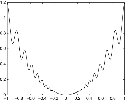
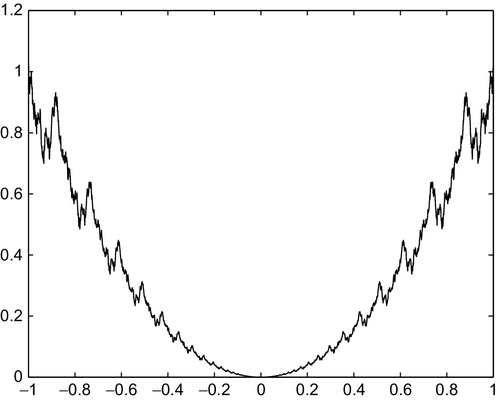
Figure 3.2 shows graphs of b₂(r; p) = C₁r²[1 + C₂b₀(r; p)] with b₀ defined by Eq. (3.113), i.e., the sine log-periodic (smooth) PH parabola, for the following parameters:

$p=1.2;\epsilon =0.2;R=0.5;\text{Ψ}=\pi /2;C_1=1;C_2=0.2.$

4.3.3 Fractal PH Surfaces

The concept of self-affine fractals is often mentioned in studies of the roughness of surfaces. A number of experimental investigations claim that profiles of vertical sections of real surfaces are statistically similar to themselves under repeated magnifications; however, the profile should be scaled differently in the direction of the nominal surface plane and in the vertical direction. In mathematics, self-affine mapping on a plane means a one-to-one mapping such that images of any three collinear points are collinear in turn. However, in the literature devoted to fractals, self-affine mapping usually means a particular case; namely, quasi-homogeneous (anisotropic) coordinate dilation, x′ = λx and y′ = λ^H_y, where H is some scaling exponent. Since homogeneous coordinate dilation (geometrical similarity) is a particular case (λ = λ₁ = λ₂) of quasi-homogeneous dilation, it is often claimed that surfaces are self-similar. Alternatively, fractal roughness is self-similar if it looks approximately the same over some range of scales.

The Takagi-Hopson function is a Weierstrass-type function. It can be taken as an example of a fractal PH function. Its equation is as follows:

$\begin{array}{ll}{b}_d\left(r;p\right)\hfill & =C_1{r}^d\left[1+C_2{b}_0\left(r;p\right)\right],b_0=-\left(b_0^{\left(0\right)}-M\right)/A,\hfill \\ h\left(p^{n}r\right)\hfill & =2\left|p^{n}r-\left[p^{n}r+\frac{1}{2}\right]\right|,\hfill \end{array}$

where A = (max b⁽⁰⁾₀ − min b⁽⁰⁾₀)/2, M = (max b⁽⁰⁾₀ + min b⁽⁰⁾₀)/2, and

$b_0^{\left(0\right)}\left(r;p\right)=r^{-\beta }{\displaystyle \sum _{n=-\infty }^{\infty }{p}^{-\beta n}h\left(p^{n}r\right)}.$

Figure 3.3 shows a graph of the Takagi-Hopson fractal PH parabola b₂(r; p) for the same values of the parameters as for the smooth PH parabola. The box-counting dimension of graphs of the Weierstrass-type functions and the PH functions b⁽⁰⁾₀ and b₂ above are the same and equal to (2 − β). An extended discussion of fractal PH functions was given by Borodich (1996, 1998a, 1998b).

It is almost evident that the problem of indentation of a continuous half-space by a conical or wedge-shaped punch is self-similar owing to the condition of geometrical similarity of the indenter. The first attempts to study the similarity of the problem were made in the nineteenth century (for details, see Grigorovich, 1976). Then dynamical problems of indentation of a fluid half-space by a wedge-shaped punch were studied by Karman and Wattendorf (1929), Wagner (1932), and others (for details, see Borodich, 1988a). To the best of my knowledge, Hill et al. (1947) presented the first rigorous application of similarity methods to the contact problem in solid mechanics. They studied the problem of contact between a wedge-shaped punch and a rigid-perfectly plastic half-space (Hill et al., 1947; see also Hill, 1950; Johnson, 1985). Note the formulation of the above contact problem for the rigid-perfectly plastic half-space differs from the formulation of the Hertz contact problem.

4.4.2 Contact with Isotropic Elastic Media

To the best of my knowledge, the idea to apply similarity arguments to axisymmetric Hertz contact problems for linear elastic isotropic bodies goes back to Mossakovskii (1954) and Landau and Lifshitz (1954, 1959). Using the explicit Hertz solution of the problem for two contacting, linear elastic spheres, Landau and Lifshitz applied some similarity arguments to show that a relation between the relative approach of the spheres’ centers (δ) and the compressing load (P) of the form

$\delta =\text{const}\times P^{2/3}$

holds not only for spheres but also for other finite contact bodies. Then Kilchevskii (1960) showed this conclusion can be obtained without the assumption that the contact region is either a circle or an ellipse. Similarity arguments were applied to some axisymmetric nonslipping contact problems for linear elastic isotropic bodies. Spence (1968) developed the results presented by Mossakovskii (1954, 1963) and showed that for an axisymmetric indenter described by a power-law function, the solution of the Hertz problem with nonslipping boundary conditions is self-similar. Spence (1975) also considered self-similar axisymmetric frictional Hertz problems.

At the beginning of 1980s, two self-similar approaches to 3D contact problems were proposed independently. The self-similarity of 3D Hertz-type contact problems for an isotropic linear elastic material was shown by Galanov (1981b) and Borodich (1983).

The approach developed by Galanov is based on the use of the solution to the Boussinesq problem for a normal concentrated load. By 1982, Galanov (1981b, 1982) had shown self-similarity of the Hertz-type contact problems not only for isotropic linear elastic solids but also for nonlinear plastic and linear viscoelastic materials.

The approach introduced by Borodich (1983, 1988b, 1989, 1990e) deals directly with the equations of the formulation of a Hertz-type boundary value contact problem and an analysis if the solution can be described by quasi-homogeneous functions. First, this approach was applied to the 3D contact problem for isotropic linear elastic bodies and to the problem of Hertzian elastic collision (Borodich, 1983). Then this approach was developed further and applied to a nonclassic contact problem for distorted half-spaces whose initial gap is described by a homogeneous function of negative degree (Borodich, 1984, 1996). A particular case of the latter class of problems is a problem of contact between two elastic half-spaces that are disjoint by two opposite concentrated loads applied at the coordinate origin, and pressed against each other by some constant pressure applied at infinity. In this problem d = −1 because as, one can see from Eq. (3.28), the distance between the distorted elastic half-spaces can be described by the function f = C/r, where C is a constant.

To explain Galanov’s approach, let us consider the following example of the contact problem formulation for a half-space whose material is incompressible and is described by the isotropic deformation theory of plasticity with constitutive relation (Eq. 3.102) assuming 0 < κ ≤ 1 (Galanov, 1981a). Using Kuznetsov (1962) representation of the solution to the Boussinesq problem for a concentrated load acting on such a material, Galanov gave the following formulation of the problem. The unknown quantities p(M), G, and δ should be found from the following nonlinear system:

$D{\displaystyle {\int }_G\frac{p\left(N\right)}{R_{\mathit{MN}}^{2-\kappa }}\text{d}{s}_N={\left(f\left(M\right)-\delta \right)}^{\kappa }};{\displaystyle {\int }_{G}p\left(N\right)d{s}_N=P};p\left(M\right)\le 0;p{\left(M\right)|}_{\partial G}=0;M\left(x,y\right),N\left(\xi ,\eta \right)\in G,$

where R_MN is the distance between points M and N, p(M) is the contact pressure, and D is a constant depending on κ and A.

Using the above formulation, Galanov (1981a) proved that the problem of contact between a punch whose shape is described by a homogeneous function with d ≥ 1 and a half-space whose material has constitutive relation (Eq. 3.102) is self-similar. Hence, it can be treated as a steady-state problem. The problem was solved numerically. Galanov (1981a) provided a justification of the numerical approach used. Actually he formulated and proved a theorem saying that for the load P → ∞, the change of the stresses at any point of the half-space in the above contact problem is equivalent to a progressive change along a straight line in the stress space. This theorem shows that the contact problem can be treated as a problem of the isotropic deformation theory of plasticity with power-law hardening, and hence his approach is justified. Unfortunately many papers devoted to indentation of elastic–plastic materials do not give such a theoretical justification for the numerical schemes employed, and instead of the use of proper constitutive relations (Eq. 3.7), they consider only one-dimensional stress-strain relations like Eq. (3.95).

Galanov (1981a) considered not only progressive loading of the isotropic elastic–plastic material but also linear unloading. Hence, he considered a truly elastic–plastic contact problem and described the profile of the imprint after removal of the indenter (Galanov, 1981a, 2009). However, if one does not consider unloading, then the above problem can be treated as a problem for a nonlinear elastic material (Borodich, 1989, 1990e). The similarity approach used later by Hill et al. (1989) is similar to the approach used by Galanov; however, they considered only the problem for loading.

Comments.

1. One has to realize that solving problems for materials with power-law hardening stress–strain relations is a very difficult task. For example, some features of Kuznetsov’s solution do not have any physical meaning, e.g., D used in Eq. (3.115) is negative for 0 < κ < 2/3 and is positive for all other values from the unit interval. The value of the coefficient c can be obtained by solving a fourth-order nonlinear ordinary differential equation. Because no analysis of the equation was presented by Kuznetsov (1962), Galanov (1984) solved the equation numerically for 0 < κ ≤ 1 and found the values of c.

2. Galanov and Kravchenko (1986) considered self-similar contact problems for isotropic creeping materials with constitutive Eqs. (3.106) and (3.107). They used an integral formulation similar to Eq. (3.115). Their formulation was based on an approximate principle of superposition of “generalized displacements” introduced by Arutyunyan (1967):

${\left(u_3\right)}^{\kappa }=D\frac{P}{R_{\mathit{MN}}^{2-\kappa }}.$

Such an approximation was introduced because formally one cannot use a superposition for a nonlinear material.

3. Svirskii (1984) considered problems for concentrated loads applied, respectively, vertically or horizontally to the boundary plane of a physically nonlinear compressible half-space whose material obeys the law of power-law hardening, i.e., he considered analogies to the Boussinesq and Cerruti problems (see, e.g., Lurie, 2005). He assumed that shear stresses τ_rɸ = τ_ɸθ = τ_rθ = 0, and hence the stresses in the half-space are defined solely by the field of normal stresses that satisfy the constitutive relations σ_i = Aε^κ_i, where σ_i and ε_i are the intensities of the stress and strain tensors, respectively, and A is a material constant. In addition, he used the above-mentioned Arutyunyan principle of superposition of “generalized displacements.” Svirskii (1984) obtained an exact analytical solution of these problems and derived another value for the constant D:

$D=3^{\left(\kappa +1\right)/2}\left(\frac{\kappa +2}{6\pi A}\right){\left[\frac{{\kappa }^2}{2\left(4-{\kappa }^2\right)}\right]}^{\kappa },0<\kappa \le 1.$

4.4.3 Contact with Viscoelastic and/or Anisotropic Elastic Media

It was shown that the approach which deals with the equations of elasticity directly can be applied to the frictionless contact problems for anisotropic linear elastic materials (Borodich, 1990d, 1990e), anisotropic linear viscoelastic materials, i.e., materials with constitutive equations (Eq. 3.105), anisotropic nonlinear elastic materials, i.e., materials whose elastic energy U is a homogeneous function of degree k + 1 in terms of ε_ij (see Borodich, 1988b, 1989, 1990e), and an anisotropic elastic half-space with initial stresses (Borodich, 1990a). Hill et al. (1989) considered axisymmetric Hertz-type contact problems for anisotropic nonlinear elastic materials.

Then it was shown by Borodich (1993a) that the similarity approach is valid for all the above problems with nonslipping (Eq. 3.14) or frictional (Eq. 3.15) boundary conditions.

As already mentioned, if a contact problem is self-similar, then this non-linear problem can be solved only for one value of the external parameter, while the solutions for all other values can be obtained by elementary recalculations. Galanov (1981a, 1981b) was the first to develop effective numerical schemes using a self-similar property. Then Hill et al. (1989) developed other schemes for numerically solving self-similar problems.

Galanov (1981a) applied the similarity approach to isotropic plastic materials (see also Borodich, 1990e, 1998c). Later the similarity properties of this problem were used by Biwa and Storåkers (1995).

Then Galanov applied his approach to isotropic viscoelastic materials (Galanov, 1982). Note that his results are also valid for some inhomogeneous materials; namely, materials whose viscoelastic properties are power-law functions of the depth. Finally, self-similar contact problems for isotropic creeping materials with constitutive Eqs. (3.106) and (3.107) were considered by Galanov and Kravchenko (1986). Hence, Galanov and his coworkers described practically all cases of self-similar frictionless Hertz-type contact for isotropic media. After 1986 it was interesting to develop the similarity approach to contact problems for nonlinear anisotropic bodies. The first results in this field were announced by Borodich (1988b, 1989). The detailed studies of similarity in 3D contact problems for anisotropic nonlinear plastic materials (constitutive Eqs. 3.102 and 3.103), hereditarily elastic materials (constitutive Eq. 3.108), and anisotropic nonlinear creeping solids (constitutive equations of Eq. 3.110 type) were published in 1990 (Borodich, 1990b, 1990c, 1990e).

Independently, Hill (1992) applied the similarity approach to consider axisymmetric Hertz contact problems for nonlinear creeping solids. Later this problem for materials with constitutive equations of Eq. (3.109) type was studied both theoretically and numerically by Bower, Fleck, Needleman, and Ogbonna (1993) and Storåkers and Larsson (1994). Then the 3D problems were considered by Storåkers, Biwa, and Larsson (1997).

Galanov (2009) noted in his review that the similarity approach gives not only theoretical rescaling formulae for microindentation and nanoindentation tests but also helps to understand the correlation of basic parameters of contact interaction and the specific nature of the indentation tests.