
4.5 General Similarity Transformations
4.5.1 Similarity Transformations of Contact Regions
The following condition has to be fulfilled for the contact problem to be self-similar: the contact region for one value of the external parameter has to be geometrically similar to the contact region for any other admissible value of the parameter. It is well known from mathematics (group theory) that any similarity transformation on a plane can be decomposed into four transformations: (1) shifting; (2) rotation; (3) dilation of coordinates; and (4) mirror symmetry. The reduction of variables using the Π theorem and reduction of variables using the property of quasi-homogeneous functions are possible if the dilation transformation of variables is used. It is evident that if a contact region has some axes of geometrical symmetry, then the use of mirror symmetry and rotation of the computation domain can be used for simplification of the numerical simulations; however these transformations should be excluded from the consideration as transformations of the contact region due to a change of the problem external parameter, because they have no physical meaning for contact problems.
Let us show that the problem of oblique indentation cannot be analyzed solely by the use of reduced coordinates (rescaling). Indeed, in the problem of oblique indentation, the nose of the indenter is shifted along the x3 = 0 plane. However, if the growing contact region is geometrically similar to itself at an earlier stage and the center of the region is shifted, then two transformations are involved: shifting and dilation of coordinates. On the other hand, the use of reduced coordinates (rescaling) is applicable to the transformation of dilation of coordinates when the contact region is not shifted. Therefore, one cannot reduce the problem of oblique indentation to dilation with the fixed coordinate origin and use the reduced variables.
It should be noted that if one considers contact between axisymmetric bodies whose materials are isotropic or they satisfy the condition of rotational symmetry, then the problem has some self-similar features even if its solution is not self-similar. Indeed, the contact region is always a circle, i.e., it is changed by the homothetic transformation. However, the problem is more complicated for arbitrary 3D shapes or for general anisotropy of materials. Indeed, in contrast to the isotropic case, if a body of revolution contacts with an anisotropic medium, then the contact region can be noncircular. For example, it was experimentally observed in the problem of indentation of an anisotropic wooden specimen (balsa wood, 67% saturation) by a spherical indenter that the contact region differs from a circle and is close to an ellipse (Bowden & Tabor, 1964). However, even in this case the similarity approach based on the use of the dilation transformation of variables is still valid.
4.5.2 Dilation Similarity Transformations of Hertz-Type Contact
It was shown by Borodich (1989, 1990e, 1993a) that if one punch is replaced by another one using the following transformations then one solution of the contact problem can be transformed into another solution. Implicitly the transformations were used earlier (Borodich, 1984).
Transformation A. The function of the shape of the punch is transformed by homogeneous dilations λ along all axes, i.e.,
In this case, the punch is replaced by its scaled copy (see Fig. 3.4).

Transformation B. The function of the shape of the punch is transformed by dilation λ along the x3 axis only, i.e.,
In this case, the punch is replaced by another one whose shape is just an extension along the x3 axis of the original shape (see Fig. 3.5).

4.5.3 Similarity Theorems of Hertz-Type Contact
Theorem 3
(similarity I). Let f1 be an arbitrary positive function of the blunt punch shape. Let the punch be pressed in a continuous half-space, whose operator of constitutive relations F is arbitrary. Let the functions u*i(x, t, P0) and σ*ij(x, t, P0), the quantity δ*(t, P0), and the region G*(t, P0) give the solution to the Hertz-type contact problem (3.6)–(3.12) with one of conditions (3.13)–(3.15) for this punch and a pressing force P0.
Then, the solution to this problem for another punch obtained by transformation A from the original punch, i.e., its shape is described by the function f,
and pressed in the half-space by the force
is given by ui(x, t, P), σij(x, t, P), and δ(t, P), namely,

and the contact region G(t, P) changes according to the homothetic transformation, i.e.,
Corollary. If one looks for the punch shape such that it transforms under transformation A into itself, then it is readily seen that this is a 3D cone, B1(θ)r.
Theorem 4
(similarity II). Let f1 be an arbitrary positive function of the blunt punch shape. Let the punch be pressed in a nonlinear half-space with the operator F satisfying Eq. (3.100). Let the functions u*i(x, t, P0) and σ*ij(x, t, P0), the quantity δ*(t, P0), and the region G*(t, P0) give the solution to the Hertz-type contact problem (3.6)–(3.12) with one of conditions (3.13)–(3.15) for this punch and a pressing force P0.
Then, the solution to this problem for another punch obtained by transformation B from the original punch, i.e., its shape is described by the function f,
and pressed in the half-space by the force
is given by ui(x, t, P), σij(x, t, P), and δ(t, P), namely,

and the contact region G(t, P) is the same, i.e.,
One can see that the contact region is not changed under transformation B. Let us unify these two transformations. In this case the function of the shape f1 of the punch is transformed by dilation λ1 along the x1 and x2 axes and by λ2 along the x3 axis, i.e., the function of the shape f of the transformed punch is given by
Then a formulation of the following theorem of similarity can be given.
Theorem 5
Let f1 be an arbitrary positive function of the blunt punch shape. Let the punch be pressed in a nonlinear half-space with the operator F satisfying Eq. (3.100). Let the functions u*i(x, t, P0) and σ*ij(x, t, P0), the quantity δ*(P0), and the region G*(P0) give the solution of the Hertz-type contact problem (3.6)–(3.12) with one of conditions (3.13)–(3.15) for this punch and a pressing force P0.
Then, the solution of this problem for another punch, whose shape is described by the function f satisfying Eq. (3.115) and which is pressed in the half-space by the force
is given by ui(x, t, P), σij(x, t, P), and δ(t, P), namely,
and the contact region G(t, P) changes according to the homothetic transformation, i.e.,
Remarks.
1. Formally, Theorem 5 would be valid for other conditions of friction within the contact region, in particular conditions when regions of stick and slip are alternating. However, these conditions look rather unreal.
2. Theorem 5 shows that there exists a two-parameter transformation group of coordinate dilations such that it transforms one solution to the problem into another one. So, it gives a mathematical explanation for the existence of the similarity which was considered in papers where the distance between contacting bodies was determined by a positive, homogeneous function of degree d ≥ 1. Indeed, if the punch shape is described by a homogeneous function, then the two-parameter transformation group becomes a one-parameter transformation group and the punch under the considered transformation of coordinate dilation is transformed into itself. Thus, taking λ1 = λ−1 and λ2 = λ−d, one obtains the following theorem of similarity.
Theorem 6
Let the shape of a blunt punch be determined by a positive, homogeneous function of degree d > 0. In addition, let the operator of the constitutive relations F satisfy Eq. (3.100).
Assume further that for a value of the compressing force P0 the solution of the Hertz-type contact problem (3.6)–(3.12) with one of conditions (3.13)–(3.15) is given by the functions σij(x, t, P0), εij(x, t, P0), and ui(x, t, P0), quantity δ(t, P0), and regions G(t, P0) and G1(t, P0).
Then, for any positive force P the solution of the boundary value contact problem is given by

where λ = (P0/P)1/[2+κ(d−1)], i.e., P0 = λ[2+κ(d−1)]P, and the contact regions G(t, P0) and G1(t, P0); G(t, P0) ⊇ G1(t, P0) change according to the homothetic transformation, i.e.,
The similarity properties of all Hertz contact problems considered follow from Theorem 6 (see, e.g., Biwa & Storåkers, 1995; Borodich, 1988b, 1990a, 1990b, 1990c, 1990d, 1990e, 1993a; Galanov, 1981a, 1981b, 1982; Galanov & kravchenko, 1986; Hill et al., 1989).
Similarly to the case of the Hertz contact, the following theorem can be proved (Borodich, 1996, 1998a).
Theorem 7
Let the shape of a blunt punch be determined by a positive PH function of degree d > 0 and parameter p.
In addition, let the operator of the constitutive relations F satisfy Eq. (3.100). Assume further that for every value of compressing force P0 on the half-interval (P1, p[2+κ(d−1)] P1] the solution of the contact problem (3.6)–(3.12) and (3.13) or (3.14) is given by the functions σij(x, t, P0; p), εij(x, t, P0; p), and ui(x, t, P0; p), quantity δ(t, P0; p), and region G(t, P0; p).
Then, the boundary value contact problem for each force P is satisfied by

and the contact region G(t, P0; p) changes according to the homothetic transformation, i.e.,
where ![]() , k0 ∈ Z, i.e. the set of integer numbers.
, k0 ∈ Z, i.e. the set of integer numbers.
As already mentioned, the PH function b0 can be fractal. However, even for such a fractal punch, the shape function f = b2(x; p) = C1x2 [1 + εb0(x; p)] has the derivative at the origin, f′(0) = 0. So, we can assume that the formulation of the contact problem is still valid for these fractal punches, and therefore Theorem 7 is also valid in the fractal case.
Often mathematical and physical fractals are confused and theorems proved for mathematical fractals are transferred without any adjustment to physical objects. One needs to realize that physical fractals exhibit the power-law behaviour only at intermediate scales δ, while mathematical ones assume that fractal dimension values of a set have to be calculated when δ → 0. This is one of the principal distinctions between physical and mathematical fractals. Hence, there are no mathematical fractals in nature. A mathematical fractal is just one of the possible models that reflect the power-law behavior of natural objects at some intermediate scales. It is wrong to expect that modeling of a rough surface by a mathematical fractal gives considerable advantages in studying an engineering problem. For these fractal curves or surfaces, one cannot use, at least in the usual sense, such a common notion as a normal vector to the surface. Hence, it is impossible to use the classic formulation of boundary value problems for a solid with mathematical fractal boundaries (Borodich, 2013).
It is evident that the solution to the contact problem for a PH punch has discrete self-similar properties, i.e., it is repeated in scaling form near all loads ![]() . Hence, it is possible to get the whole solution using the results of numerical simulation of the problem on a finite half-interval of external parameter (the so-called fundamental domain of the discrete group) only. In the above case, this fundamental domain is (P1, p[2+κ(d−1)] P1].
. Hence, it is possible to get the whole solution using the results of numerical simulation of the problem on a finite half-interval of external parameter (the so-called fundamental domain of the discrete group) only. In the above case, this fundamental domain is (P1, p[2+κ(d−1)] P1].
It follows from Theorem 7 that the character of the contact does not depend on fine distinctions between shapes and the roughness functions b0. The character of the self-similar solution depends on the degrees of homogeneity of the PH function of the punch shape and the operator F only. Thus, the solutions for all PH punches of degree d have the same character. One can conclude that the nonadhesive contact problems with PH roughness have some features of chaotic systems: the trend of the P-δ curve (the global characteristic of the solution) is independent of fine distinctions between PH functions describing roughness, while the stress field (the local characteristic) is sensitive to small perturbations of the punch shape. In particular, the character is the same for both fractal (prefractal) and smooth functions b0. Particular cases of Theorem 7 in application to PH surfaces were considered by Borodich (1993b, 1998a) and Borodich and Galanov (2002).
4.6 Rescaling Formulae and Indentation Tests
4.6.1 General Rescaling Formulae
It follows from similarity analysis of self-similar nonaxisymmetric contact problems that if the contacting pair is loaded by the force P1, and the characteristic size of the contact region and the approach of solids are known for this load, they are equal to l(1, t, P1) and δ(1, t, P1) respectively. Then for the contact pair compressed by some force P, and whose initial gap is described by the function chd, c > 0, the size of the contact region and the approach may be defined by the following rescaling formulae:

As mentioned above, these formulae provide an explanation for the Meyer scaling law.
4.6.2 Rescaling Formulae for Hardness and Nanoindentation
Let us denote by P1, A1, l1, and δ1, respectively, some initial load, the corresponding contact area, the characteristic size of the contact region, and the displacement. Then Eq. (3.116) can be rewritten as

and as shown by Borodich et al. (2003), the rescaling formula for the contact area is
Further, for a fixed indenter, i.e., for c = 1, one can find that the hardness is the following function of the depth of indentation:

Thus, for a fixed indenter, whose shape near the tip is described as a monomial function of degree d, one obtains from Eqs. (3.118) and (3.119)
Note that the fist of the relations in Eq. (3.120) is valid independently of the work-hardening exponent κ. The apparent hardness increases as a power-law function of degree κ(d − 1)/d and the hardness is constant only for d = 1, i.e., for ideally sharp 3D conical (conical or pyramidal) indenters.
Using Eq. (3.118), one can try to calibrate the indenter tip from an area-displacement curve. An example of such a curve was given by Doerner and Nix (1986). Applying formula (3.120) to this curve, Borodich et al. (2003) concluded that until about δ ≤ 90 nm the shape of the indenter used by Doerner and Nix (1986) could be described as a monomial function of degree d = 1.44.
The rescaling formulae (3.117), (3.118), and (3.120) were obtained assuming the homogeneity of material properties and that the stress–strain relation remains the same for any depth of indentation. This is not always true (see, e.g., a review by Ioffe, 1949). In addition, as already mentioned, plastic deformation exhibits a strong dependence on size below micrometer length scales (Gao et al., 1999), and models of indentation hardness based on the strain gradient plasticity (Nix & Gao, 1998) predict the hardness decreases as the depth of indentation increases. However, as we have already seen, nonideal indenter geometries (Borodich et al., 2003; Choi & Korach, 2011; Kindrachuk, Galanov, Kartuzov, & Dub, 2006; Kindrachuk et al., 2009; Ma, Zhou, Lau, Low, & deWit, 2002) may also affect the interpretation of the experimental results. I believe that two explanations are possible: (1) the hardness may decrease in accordance with Eq. (3.93) if dislocation scale effects are present and (2) the apparent hardness may increase according to Eq. (3.120) because the nominally sharp indenters are in fact not ideal. However, the former case is less common because not all materials are crystalline.
4.7 Comparison with Some Experimental Data
4.7.1 The Power-Law Exponent for Poly(Methyl Methacrylate)
First, let us compare formulae (3.116) or formula (3.99) with experimental results obtained by Orlov and Pinegin (1971) for a polymeric material. Several terms are used in reference to this material: poly(methyl methacrylate), Plexiglas, and Perspex.
It is well known that poly(methyl methacrylate) is a viscoelastic (or hereditarily elastic) material. If one uses the homogeneous relations (3.106) and (3.107)

or the anisotropic homogeneous relations (3.108)

as the constitutive relations for poly(methyl methacrylate), then one needs to take into account the following. The kernel K of the constitutive relations may be singular; in this case the diagram σ ~ ε obtained by the use of common experimental techniques would differ from the instantaneous diagram φ[Γ(t)]. The difference may be considerable even if the loading time is of the order of 0.1 s (Rabotnov, 1980). However, to apply formulae (3.116) or formula (3.99), one needs to know only the power κ. Assuming the instantaneous diagram can be obtained from experiments on very fast loading, one can take the results of dynamical experiments on poly(methyl methacrylate) (Perspex) presented by Kolsky (1949). Taking logarithms of the first nine points of the dynamic strain-stress curve and using the least-squares method for a direct line in the logarithmic coordinates, one can obtain κ = 0.7202 (Borodich, 1990e).
4.7.2 Variation of the Loading Time
Owing to viscoelasticity of the material, the characteristic size of the contact region depends on time. Table 3.1 shows the experimental relation between the diameter of the contact region l(P) = 2a and time for a spherical steel indenter of R = 60 mm under P1 = 500 kgf and P2 = 1000 kgf (Orlov & Pinegin, 1971, p. 53). If one takes κ = 0.7202 for poly(methyl methacrylate), then the formula (3.99) can be written as

Table 3.1
Comparison of the Experimental Results and the Rescaling Values Obtained by Eq. (3.121) for Distinct Values of Time
| l(P)/t | 1 s | 5 s | 10 s | 60 s | 600 s | 1800 s |
| P1 = 500 kgf | 8.0 | 8.40 | 8.70 | 8.85 | 8.90 | 8.95 |
| P2 = 1000 kgf | 10.55 | 10.65 | 10.75 | 11.10 | 11.50 | 11.78 |
| Formula (3.121) | 10.32 | 10.84 | 11.22 | 11.42 | 11.48 | 11.55 |
| Error Δ, % | 2.2 | 1.76 | 4.42 | 2.87 | 0.15 | 1.97 |
The error is found as

One can see that there is excellent agreement between the experimental data and the predictions by Eq. (3.99) or Eq. (3.121).
4.7.3 Variation of the Indenter Size and the Load
Earlier, formula (3.99) was compared with data concerning indentation of an anisotropic wooden specimen by a spherical indenter (Bowden & Tabor, 1964). It was shown by Borodich (1989, 1990e, 1993a) that there is good agreement between experiments and the formula.
It is possible now to check if Eq. (3.99) is in agreement with experiments performed by Orlov and Pinegin (1971, p. 54).
The measurements were taken for a relatively fast loading, i.e., t was approximately 1 s or less. The loads were given in kilogram-force. It was taken that 1 kgf ≈ 10 N because this rounding will not affect the calculations since only the ratio P/P1 is used in Eq. (3.99).
To use the rescaling formulae, one needs to know a solution (or an experimental result) for a certain value of the external parameter. It was taken that l(R1, P1) = 11.3 mm for the load P1 = 12.9 kN, and that the sphere had radius R1 = 38.1 mm (or D1 = 76.2 mm) as presented by Orlov and Pinegin (1971, p. 54). Hence, only one experimental measurement was used to obtain all rescaling values in Table 3.2. One can see that formula (3.99) describes the experiments quite well.
Table 3.2
Comparison of the Experimental Results and the Rescaling Values Obtained by Eq. (3.99)
| Diameter (mm) | Load (N) | Diameter of Contact Region (mm) | Diameter of Contact Region by Formula (3.99) | Error (%) |
| 15 | 1000 | 2.7 | 2.87 | 6.3 |
| 1500 | 3.3 | 3.33 | 0.95 | |
| 2000 | 3.6 | 3.7 | 2.87 | |
| 3000 | 4.3 | 4.3 | 0.03 | |
| 4000 | 4.9 | 4.78 | 2.49 | |
| 5000 | 5.4 | 5.19 | 3.95 | |
| 22.1 | 2200 | 4.1 | 4.25 | 3.65 |
| 3300 | 4.75 | 4.93 | 3.85 | |
| 4300 | 5.3 | 5.44 | 2.58 | |
| 6500 | 6.3 | 6.33 | 0.46 | |
| 8700 | 7.1 | 7.04 | 0.78 | |
| 10,800 | 8.0 | 7.63 | 4.66 | |
| 31.75 | 4500 | 5.9 | 6.09 | 3.14 |
| 6700 | 7.2 | 7.04 | 2.17 | |
| 9000 | 7.8 | 7.85 | 0.66 | |
| 13,400 | 9.4 | 9.09 | 3.32 | |
| 17,900 | 10.7 | 10.11 | 5.5 | |
| 22,400 | 11.8 | 10.98 | 6.97 | |
| 76.2 | 12,900 | 11.3 | 11.3 | 0 |
| 15,500 | 12.0 | 12.09 | 0.74 | |
| 20,600 | 13.6 | 13.42 | 1.31 | |
| 25,800 | 14.8 | 14.58 | 1.49 | |
| 38,700 | 16.7 | 16.92 | 1.34 |

5 Axisymmetric adhesive contact problems
5.1 Molecular Adhesion and Its Modeling
5.1.1 Basic Terminology
Adhesion and adhesive contact problems have been studied for a long time. Adhesion is a universal physical phenomenon that usually has a negligible effect on surface interactions at the macroscale, whereas it becomes increasingly significant as the contact size decreases (Kendall, 2001). The term “adhesion” may have rather different meanings. It may be used to denote both the strong chemical bonds between surfaces and weak connections due to van der Waals forces. Other physical mechanisms of adhesion (e.g., adhesion due to electrical double layer charges) are also possible (Deryagin, Krotova, & Smilga, 1978). In addition, contact problems with nonslipping boundary conditions are often called adhesive contact problems (Mossakovskii, 1963; Spence, 1968).
Here forces of chemical bonding are not studied, and only molecular adhesion caused by van der Waals forces is considered. The distinction of these forces is somewhat artificial, because all of these forces are electrical in nature (Deryagin et al., 1978; Kiselev, Kozlov, & Zoteev, 1999; Parsegian, 2005); however, this distinction is very convenient because the interaction energies are rather different. The same distinction is usually introduced for studying phenomena of adsorption of a single molecule to a surface, where it is customary to divide adsorption into physical adsorption (physisorption) and chemisorption. The binding forces for physisorption are relatively weak, while the term “chemisorption” is used if the adsorption energy is large enough to be comparable to chemical bond energies. To study contact problems with molecular adhesion, one needs to know the work of adhesion w, which is equal to the energy needed to separate two dissimilar surfaces from contact to infinity (if the materials are identical, then adhesion is called cohesion). In other words, w is the work of adhesion that is equal to the tensile force integrated over the distance necessary to pull the two surfaces completely apart (Harkins, 1919).
5.1.2 Historical Preliminaries
Apparently, the first scientific discussion of the adhesion phenomenon is due to Robert Hooke. Observing liquors, syrups, and other “tenacious and glutinous bodies,” he wrote (Hooke, 1667) “it is evident, that the Parts of the tenacious body, as I may so call it, do stick and adhere so closely together, that though drawn out into long and very slender Cylinders, yet they will not easily relinquish one another… And this Congruity (that I may here a little further explain it) is both a Tenaceous and an Attractive power; for the Congruity, in the Vibrative motions, may be the cause of all kind of attraction, not only Electrical, but Magnetical also, and therefore it may be also of Tenacity and Glutinousness“.
In 1873 van der Waals discovered a property of molecules to attract each other and wrote that he had “come to the conclusion that attraction of the molecules decreases extremely quickly with distance, indeed that the attraction only has an appreciable value at distances close to the size of the molecules“ (van der Waals, 1910). Maxwell (1874) gave a very great appraisal of the van der Waals results and agreed that attraction is considered at short distances, but that molecules repel each other on a closer approach. Peter Lebedev gave the first electromagnetic explanation for van der Waals forces (Lebedew, 1894). However, only after the introduction of quantum mechanics by M. Planck were modern descriptions of the various kinds of attractive forces given by Debye, London, and Keesom (Parsegian, 2005). The attractive forces are collectively called van der Waals forces. The term includes attraction between two permanent dipoles (Keesom force), a permanent dipole and a corresponding induced dipole (Debye force), and two instantaneously induced dipoles (London dispersion force).
5.2 Models of Adhesive Contact
5.2.1 Adhesion Between Rigid Spheres
Bradley (1932) was the first to conside attraction between two absolutely rigid spheres. Taking into account only one of the components of the van der Waals forces, namely, the London dispersion force, he calculated pointwise the attraction of each point of one sphere to another one. Assuming additivity of the London forces, he calculated the total adhesive force between the spheres Pc. Although strictly speaking the London forces are not additive (Derjaguin, Abrikosova, & Livshitz, 1958), the assumption of additivity of the forces is usually considered as acceptable (Deryagin et al., 1978).
In 1934 Derjaguin published a series of papers (see, e.g., Derjaguin, 1934a, 1934b) where he studied the influence of adhesion on friction and contact between elastic solids. Developing his molecular theory of external friction, Derjaguin (1934a) referred to results of W Hardy from 1922, K. Terzagh from 1925, and G. Tomlinson from 1929; and developing his theory of adhesion, Derjaguin (1934b) referred not only to Tomlinson but also to Bradley (1932). Derjaguin (1934b) pointed out that to calculate adhesive interactions between particles, one needs to take into account the deformations of the particles. Derjaguin (1934b) presented the first attempt to consider the problem of adhesion between elastic spheres or between an elastic sphere and an elastic half-space. He assumed that the deformed shape of the sphere can be calculated by solving the Hertz contact problem, and suggested calculating the adhesive interaction by using only attraction between points at the surfaces of the solids and by introduction of the work of adhesion (this is the so-called Derjaguin approximation).
In fact, the Derjaguin approximation (see Derjaguin, 1934b, p. 156) can be formulated as follows:
1. instead of the pairwise summation of the interactions between the elements of solids, the volume molecular attractions are reduced to surface interactions;
2. the surface interactions are taken into account only between the closest elements of the surfaces lying on vertical straight lines; and
3. the interaction energy per unit area between small elements of curved surfaces is the same as the interaction energy per unit area energy between two parallel infinite planar surfaces.
The expression for adhesion between rigid spheres Pc was obtained by Bradley (1932) after rather lengthy calculations. He needed to perform pointwise calculations of the London forces similar to calculations of gravitational forces by I. Newton; however, the adhesive forces did not decrease as gravitational forces, i.e., as 1/r2 (I. Newton learned of this law of gravity from a letter written by R. Hooke; see Arnold (1990)), but rather as 1/r7. The same result can be obtained in just one line using the Derjaguin approximation. Indeed, using the Hertz approximation, one can replace a sphere of radius R by a paraboloid of revolution δ = f(r) = B2r2, where B2 = 1/(2R). Then, applying the Derjaguin approximation, one obtains

Here pa(z) is the adhesive force per unit area between flat surfaces separated by a distance z.
Starting from pioneering papers of Derjaguin (1934a, 1934b), the mechanics of adhesive contact between isotropic elastic solids developed into a well-established branch of science. The Derjaguin approximation is implicitly involved in many modern models of adhesive contact (however, these assumptions are usually used without referring to Derjaguin).
5.2.2 Sperling Model of Adhesive Contact
Unfortunately, some of Derjaguin’s assumptions and calculations were not correct. For example, Derjaguin’s assumption about the shape of deformed solids was not correct (in fact, he was not consistent in application of his approach). Nevertheless, his basic argument was correct because it equated the work done by the surface attractions against the work of deformation in the elastic spheres (see Kendall, 2001, p. 183).
In 1964 Sperling presented his Ph.D. thesis devoted mainly to the development of a model of adhesion between rough particles. In his thesis, Sperling (1964) discussed not only ideas introduced by Derjaguin (1934b), Lifshiz (Derjaguin et al., 1958; Parsegian, 2005), and Rumpf (1990), but also developed statistical models of adhesive contact between rough particles and studied the influence of plastic and viscoelastic effects on adhesion. It is known (see, e.g., Rabinovich, Adler, Ata, Singh, & Moudgil, 2000) that the Rumpf model is based on an application of the Derjaguin approximation to adhesion between rough rigid particles. However, adhesion between an elastic half-space and a sphere of radius R was also studied (see Sperling, 1964, pp. 69–78). Employing the Derjaguin idea that the virtual work done by the external load is equal to the sum of the virtual change of the potential elastic energy and the virtual work that will be consumed by the increase of the surface attractions (see (21) in Derjaguin, 1934b), Sperling wrote the following expression for the total potential energy U of the contact system:
where a is the contact radius, m = 1/ν, μ is the shear modulus of the material, C is an arbitrary constant, and P is the external load. In his calculations he used the solution presented by Jung (1950).
Sperling noted that equilibrium is observed when the energy is a minimum. By differentiating Eq. (3.124), he derived the following two expressions (see (88) and (89) in Sperling, 1964):
and

Expressions (3.124) and (3.125) and the corresponding dimensionless load-displacement curve were analyzed. In particular, it was found that the maximum value of the tensile force is equal to the separation force (see (93) in Sperling, 1964)
and that at P = 0 the corresponding contact radius a0 and displacement δ0 are

Note that by using the Poisson ratio ν instead of m, one can present Eqs. (3.125) and (3.124) as
or

5.2.3 The JKR Theory of Adhesive Contact
Johnson (1958) attempted to solve the adhesive contact problem for spheres by adding two simple stress distributions, namely, the Hertz stress field to a rigid flat-ended punch tensile stress distribution. Johnson argued that the infinite tension at the periphery of the contact would ensure that the spheres would peel apart when the compressive load was removed. Although Johnson’s conclusion about impossibility of adhesive contact was not correct, his suggestion to superpose the stress fields is very fruitful.
According to Kendall (2001, pp. 185–186), the JKR theory was developed historically in the following steps. In 1970 Kendall and Roberts discussed the experimental observations that the contact spots were larger than expected from the Hertz equation. They found “that the answer lay in applying Derjaguin’s method … to Johnson’s stress distribution.” Johnson presented a mathematical realization of this idea an evening later. Johnson et al. (1971) applied Derjaguin’s idea to equate the work done by the surface attractions against the work of deformation in the elastic spheres, to Johnson’s stress superposition, and created the famous JKR theory of adhesive contact. The JKR approach is based on the use of a geometrically linear formulation of the contact problem, and a combination of both the Hertz contact problem for two elastic spheres and the Boussinesq relation for a flat-ended cylindrical indenter.
If there were no surface forces of attraction, the radius of the contact area under a punch subjected to the external load P0 would be a0, and it could be found by solving the Hertz-type contact problem. However, in the presence of the forces of molecular adhesion, the equilibrium contact radius a1 would be greater than a0 under the same force P0.
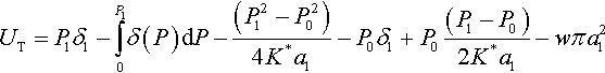
Johnson et al. (1971) suggested considering the total energy of the contact system UT as made up of three terms: the stored elastic energy UE, the mechanical energy in the applied load UM, and the surface energy US. It is assumed that the contact system has come to its real state in two steps: (1) first it has a real contact radius a1 and an apparent depth of indentation δ1 under some apparent Hertz load P1, and then (2) it is unloaded from P1 to a real value of the external load P0, keeping the contact radius a1 constant (Fig. 3.6). The Boussinesq solution for contact between an elastic half-space and a flat punch of radius a1 may be used in the latter step.

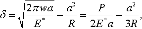
In this case, one can calculate UE as the difference between the stored elastic energies (UE)1 and (UE)2 in the loading and unloading branches, respectively. Therefore,
Using the Boussinesq solution (Eq. 3.41), we obtain for the unloading branch

Thus, the stored elastic energy UE is
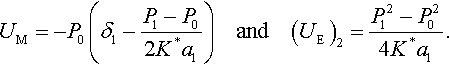
The mechanical energy in the applied load is given by
where Δδ = δ1 − δ2 is the change in the depth of penetration due to unloading.
Since only the surface adhesive interactions within the contact region are taken into account (one disregards the adhesive forces acting outside the contact region), the surface energy can be written as
The total energy UT can be obtained by summation of Eqs. (3.132), (3.133), and (3.134), i.e.,
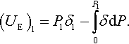
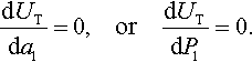
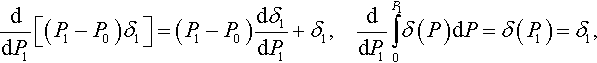
It is assumed in the JKR model that the equilibrium at contact satisfies the equation
The above was applied to the case of the initial distance between contacting solids described by a paraboloid of revolution z = r2/(2R) (this is a very good approximation for a sphere). In the framework of the JKR theory, the following relations between the external load P0 acting on the spheres and the adhesive contact radius a1 were obtained:
and
where R is the effective radius of the spheres (1/R = 1/R1 + 1/R2).
Equations (3.138) and (3.137) are exactly the same (up to the sign convention used by Sperling) as the Eqs. (3.128) and (3.129) that follows from the Sperling (1964) model. This is the reason that sometimes (see, e.g., Johnson & Pollock, 1994) the JKR theory is referred to as the JKRS theory.
It follows from the model that the instability point Pc of a P-δ curve is at the point where dP/dδ = 0, i.e.,
and dP/dδ is infinite at another special point of the P-δ curve:

Evidently Pc is the same as Fsep from Eq. (3.126) up to the sign convention used by Sperling (1964).
5.2.4 The DMT, Maugis, and Other Theories of Adhesive Contact
As mentioned above, we concentrate here mainly on the JKR theory. The theory has been very well verified for elastomers and other materials (Maugis & Barquins, 1983). However, the adhesive forces can be taken into account by various other methods, e.g., (1) by pointwise integration of the interaction forces between points of the bodies, whose interaction energy is proportional to ρ−6, where ρ is the distance between the points; (2) by using the Derjaguin approximation; (3) by introducing an interaction potential between points on the surfaces, e.g., a Lennard–Jones potential (see, e.g., Borodich & Galanov, 2004; Muller, Yushchenko, & Derjaguin, 1980); or (4) by using piecewise-constant approximations of these potentials (Goryacheva & Makhovskaya, 2001, 2008; Johnson, 1997; Maugis, 1992; Zheng & Yu, 2007).
Nowadays there are several well-established classic models of adhesive contract, which include not only the JKR theory, but also the DMT theory and the Maugis transition solution between the JKR and DMT theories (Maugis, 1992). A detailed description of the theories is given by Maugis (2000); see also discussions by Johnson (1997) and Barthel (2008). However, one could get the wrong impression that the adhesive contact problems were not studied after the publication of the papers by Bradley (1932) and Derjaguin (1934a, 1934b) until 1971, when a famous paper was published by Johnson et al. (1971). In fact, this topic was an active area of research. See, e.g., an extended review by Krupp (1967) and references in the book by Rumpf (1990).
One can see that the adhesive force (Eq. 3.139) derived by Johnson et al. (1971) does not match the value (Eq. 3.122). This fact provided a reason for Derjaguin to criticize the JKR model. Perhaps his criticism was overdone, but one has to note that Derjaguin’s papers were not cited by Johnson et al. (1971). Derjaguin et al. (1975) presented an alternative to the JKR model, and this is usually referred to as the DMT model. The difference between the JKR and DMT theories was first explained by Tabor (1977), who noted that both theories have drawbacks: the DMT theory disregards the deformations of the shape of the contacting solids near the edge of the contact region, while the JKR theory disregards the attractive forces outside the contact region. He noted also that in the JKR model the contacting solids near the edge of the contact region form a “neck,” and hence the gap increases quickly and, in turn, the attractive force decreases very quickly. Tabor introduced a parameter μ that can be used to check whether the JKR model or the DMT models is applicable. Eventually, Muller et al. (1980) agreed with Tabor’s arguments, and using numerical simulations, they showed that the JKR theory and the DMT theory are at different limits of a parameter similar to the Tabor parameter. The historical development of the DMT theory is discussed in detail by Maugis (1992, 2000), Greenwood (1997, 2007), and Barthel (2008).
Calculating the Tabor–Muller–Maugis parameter (Maugis, 1992, 2000; Muller et al., 1980; Tabor, 1977; see also Greenwood, 2007)

one can check whether μ ![]() 1, and hence if the experiment is in the range of applicability of the JKR model, or whether μ
1, and hence if the experiment is in the range of applicability of the JKR model, or whether μ ![]() 1, and hence if one needs to apply the DMT model. Here Ref is the effective radius and z0 is the equilibrium distance between atoms of the contacting pair, which is usually between 0.3 and 0.5 nm.
1, and hence if one needs to apply the DMT model. Here Ref is the effective radius and z0 is the equilibrium distance between atoms of the contacting pair, which is usually between 0.3 and 0.5 nm.
Using the Derjaguin idea that all adhesive interactions can be attributed to the surface, Muller et al. (1980) performed numerical simulations of adhesive contact using the Lennard–Jones potential. On the basis of the ideas discussed by Tabor (1977) and Muller et al. (1980), Maugis (1992, 2000) developed an analogy between the fracture mechanics approaches and the mechanics of frictionless adhesive contact. Maugis (1992) suggested modeling the attractive forces outside the contact area as a step function of some length ∇. The idea of the step-function approximation was borrowed by Maugis (1992) from Dugdale (1960). The Maugis theory considers the adhesive contact region as consisting of the following parts: in the inner part of radius a a close contact is maintained that is described by the Hertz and Boussinesq theory; in the outer part (the annulus a < r < a + ∇) adhesive attractive forces of constant intensity σ0 are acting, but there is a gap between surfaces that increases from zero to some distance h0. It is assumed that no attractive forces act in the region r > a + ∇. A very brief and precise description of the Maugis theory (the Maugis transition solution between the JKR and DMT theories) was given by Johnson (1997). As Johnson (1997) noted, to match the work of adhesion w and the maximum force σ0 with those of the Lennard–Jones potential, one has to take h0 = 0.971 z0.
In fact, Maugis (1992) did not use the Tabor parameter because he introduced the parameter λM

Maugis (2000) estimated that the DMT theory corresponds to small values of λM (λM < 0.1), while the JKR theory corresponds to large values of λM (λM > 5).
To describe a theory of adhesive contact in a dimensionless way, one needs to select characteristic scales of the contact problem for the force and the displacement at low loads and small displacements. These scales can be chosen arbitrary using the problem governing parameters w, E*, and the effective radius Ref. The conditions Pc > 0 and δc > 0 defined by Eqs. (3.139) and (3.140) can be taken as such characteristic scales. If the JKR model is employed, then the force scale Pc has a clear physical meaning: it is the theoretical absolute value of the pull-off force in the framework of the JKR model. However, for other models, it is just a scaling parameter.
Maugis (1992) showed that for each value of the parameter λM, the graph of the functional relation P–δ is situated between the corresponding graphs for the JKR and DMT theories. Hence, the above-mentioned theories of adhesive contact of spheres can be represented as a dimensionless functional P–δ relation of the following type:

where F is given by the Maugis theory, which includes the JKR and DMT theories. The Maugis parameter λM represents the most suitable theory for the contacting materials and indenters.
The original DMT model did not have such a form. However, Maugis (2000) modified it, and the functional expression (3.143) for the DMT model in Maugis’s interpretation is

The JKR model can be expressed as (Borodich et al., 2013; Maugis, 2000)

where ![]() .
.
The generality of the Maugis theory is the main reason that it is often considered as the general model of adhesive contact (Zheng & Yu, 2007; Zhou, Gao, & He, 2011). However, further generalizations are also possible. For example, Goryacheva and Makhovskaya (2008) suggested approximating the potential of the attractive forces in the outer part of the contact region as several step functions.
5.3 The Generalized Frictionless JKR Theory
With use of the expressions presented by Galin (1946, 1961), an extension of the JKR adhesive frictionless contact problem to monomial punches was first obtained by Galanov (1993) (see also Galanov & Grigor’ev, 1994). In the same year, Borodich provided another derivation of Galanov’s solution; however, it was published much later (Borodich, 2008; Borodich & Galanov, 2004). Solutions to particular cases of the problem were independently presented by Carpick, Agraït, Ogletree, and Salmeron (1996) when d is an even integer, and Maugis (2000) for a conical punch (d = 1). In fact, the solution presented by Carpick et al. (1996) may be obtained by application of the JKR approach to the expressions presented by Shtaerman (1939) (see also equation 5.20 in Johnson, 1985), while the solution presented by Maugis (2000) may be obtained by application of the JKR approach to the result obtained by Love (1939) (see a discussion by Borodich, Galanov, Prostov, & Suarez-Alvarez, 2012).
5.3.1 The JKR Theory for an Arbitrary Axisymmetric Indenter
Let us generalize the JKR model of contact with molecular adhesion and consider the case of the distances between the contacting solids being described as arbitrary convex axisymmetric functions.
For an arbitrary axisymmetric solid, one can calculate UE as the difference between the stored elastic energies (UE)1 and (UE)2 in the loading OA and unloading AB branches, respectively (Fig. 3.6). Therefore, the stored elastic energy UE is defined by Eq. (3.130), the mechanical energy in the applied load is described by Eq. (3.133), and the surface energy can be written as Eq. (3.134).
Taking into account the Boussinesq solution (Eq. 3.41), one obtains for the unloading branch
and therefore, one has
According to the Derjaguin assumptions, the adhesive interactions are reduced to the surface forces acting perpendicularly to the boundary of the half-space. The JKR theory considers only the adhesive forces acting within the contact region, which is always a circle, and the surface energy can be written as US = −π a21w. Hence, the total energy UT can be written as
or

Taking into account the expressions
and

and applying the equilibrium condition (3.136) to (3.147), one obtains

Owing to the expressions (Eq. 3.77) of Theorem 1, one obtains from Eq. (3.148) that the equilibrium condition for the general JKR model is

or
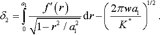
Because of Eqs. (3.146) and (3.150), one has
and hence the following expression is valid:

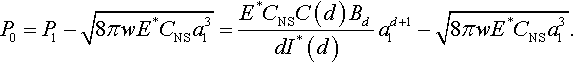
Thus, for an arbitrary convex body of revolution f(r), f(0) = 0, the general JKR theory leads to the following expressions:

Taking into account formulae (3.49) and (3.52), the relations (3.151) can be written as

and
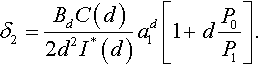
We remember that according to the notation introduced by Johnson et al. (1971), the actual force, the actual contact radius, and the actual approach between contacting bodies are denoted by P0, a1, and δ2, respectively.
5.3.2 The JKR Theory for Axisymmetric Monomial Indenters
For punches described by Eq. (3.53), the solution of the nonadhesive frictionless Hertz-type contact problem is given by
and the contact radius a1 and depth of indentation δ1 under some apparent Hertz load P1 are given by
Using Eqs. (3.154) and (3.155), one obtains an exact formula giving a relation between the real load P0 and the real radius of the contact region a1 (Borodich, 2008; Borodich & Galanov, 2004; Borodich, Galanov, Keer, & Suarez-Alvarez, 2014; Borodich, Galanov, & Suarez-Alvarez, 2014; see also Galanov, 1993):
The real displacement of the punch is δ2 = (δ1 − Δδ), i.e.,

In fact, Eqs. (3.156) and (3.157) are particular cases of Eqs. (3.152) and (3.153).
It is convenient to write the formula for the real displacement δ2 in the case of a frictionless boundary condition as

Zheng and Yu (2007) suggested writing relations (3.156) and (3.157) using the Euler beta function B(x, y) of variables x and y. Indeed, the expression (3.154) for C(d) can be written as

Then one can write


The Papkovich–Neuber formalism and the Galin solution were used in application to the mechanics of adhesive contact. In particular, Zheng and Yu (2007), Zhou et al. (2011) considered the JKR and Maugis–Dugdale contact problems for power-law-shaped solids. As Zheng and Yu (2007) noted, their solution to the JKR problem for power-law-shaped solids coincides with the solution obtained by Borodich and Galanov (2004). If one denotes Q = dBd and Δγ = w, then formulae (33) and (34) presented by Zheng and Yu (2007) in dimensional form coincide with Eqs. (3.158) and (3.159). Naturally the solution of Zhou et al. (2011) for the JKR theory coincides with the solutions by Zheng and Yu (2007) and by Galanov (1993) and Borodich, Galanov (2004). Although just the formula for the contact load was presented in the short abstract by Borodich and Galanov (2004), both formulae were presented by Galanov (1993). However, Galanov (1993) and Galanov, Grigor’ev (1994) used a different way for normalization of the variables.
Hence, for an arbitrary convex body of revolution f(r), f(0) = 0, the JKR theory leads to Eq. (3.151) or Eq. (3.152) and Eq. (3.153) (compare with previous attempts to solve this problem by Maugis & Barquins, 1983, and Maugis, 1995).
5.4 General Nonslipping Adhesive Contact
The adhesive contact problems with nonslipping boundary conditions were studied mainly in the 2D case (see, e.g., Zhupanska, 2012). However, there were also attempts to consider nonslipping adhesive contact between spheres (S. Chen & Gao, 2006; Guo et al., 2011; Waters & Guduru, 2010; Yang, Zhang, & Li, 2001). We consider below axisymmetric adhesive contact problems with nonslipping boundary conditions.
5.4.1 The Nonslipping Boussinesq–Kendall Adhesive Contact Problem
Consider an axisymmetric flat-ended punch of radius a1 that is vertically pressed into an elastic half-space. The frictionless case of this problem was considered by Boussinesq (1885), nonslipping contact was studied by Mossakovskii (1954), and frictionless contact with molecular adhesion was studied by Kendall (1971). Let us consider the problem with non-slipping boundary conditions and taking into account molecular adhesion (Borodich, 2011; Borodich, Galanov, & Suarez-Alvarez, 2014). Then the arguments of Kendall (1971) have to be slightly modified.
In this problem the boundary conditions for radial displacements within the contact region 0 ≤ r ≤ a1 have the following form:
The elastic material deforms according to the corrected Mossakovskii equation (Eq. 3.64), which can be presented as

As one can see from Eq. (3.41), the equation has the same form as the one for the frictionless case (the Boussinesq solution) with CNS equal to unity.
The surface energy is given as above by Eq. (3.134). Using Eq. (3.161), one obtains that the stored elastic energy UE and the mechanical energy of the applied load UM are, respectively,

The total energy UT can be obtained by summation of all components given by Eq. (3.134) and Eq. (3.162):

From the equilibrium equation (3.136), one has
and hence one may obtain the adhesive force (the pull-off force) of a flat-ended circular punch of radius a1 at the nonslipping boundary conditions:
Thus, one can see from Eq. (3.165) that the adhesive force is proportional neither to the energy of adhesion nor to the area of the contact. Maugis (2000) came to the same conclusion for the frictionless Boussinesq–Kendall problem.
5.4.2 Energy Approach in the Nonslipping Case
Let us calculate the total energy of the system with nonslipping conditions. As explained above, it is attempted here to follow the original JKR approach as closely as possible, avoiding the resolution of interfacial tractions. However, one needs to provide the clear rationale for the extension of the frictionless JKR approach to the case of nonslipping contact conditions. The work W of the external forces, which include the surface tractions, the body forces, and the applied load, can be written as
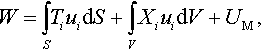
and according to Clapeyron’s theorem, it is stored in the linear-elastic body in the form of the strain energy (see, e.g., Lurie, 2005). Here Ti are the surface tractions, Xi are the body forces, and S and V are the surface and the body volume, respectively. The body forces in the problem under consideration are the adhesive forces. Because in the nonslipping case both the normal and radial tractions exist over the contact region, formally the work of radial surface tractions (UE)3 should be added to the expression for the stored elastic energy:

As already mentioned, one can use the superposition of two contact solutions for linear elastic materials if the contact region 0 ≤ r ≤ a1 is fixed. Hence, the tangential stresses in the nonslipping contact problem can be obtained as the difference between the tangential stress field τM(r) of the Mossakovskii (or Mossakovskii–Spence) type problem (this is the Hertz-type contact problem with nonslipping boundary conditions) for the punch loaded by P1 and the tangential stress field τB(r) of the Boussinesq–Mossakovskii contact problem after the unloading from P1 to P0, i.e., τ(r) = τM(r) − τB(r). Here the subscripts M and B denote variables associated with the Mossakovskii–Spence-type and the Boussinesq–Mossakovskii contact problems, respectively. Owing to the conditions (3.62), the differentials of the work done by the tangential tractions during increase of P from 0 to P1 and then during decrease from P1 to P0 are zero, and hence the work of the tangential surface tractions (UE)3 = 0.
As already mentioned, the work of the external body forces in the problem under consideration is the work done by the adhesive forces. Here it is assumed that the Derjaguin approximation is valid, i.e., the adhesive interactions are reduced to the surface forces acting perpendicularly to the boundary of the half-space, and therefore the work of the surface adhesive forces on radial displacements is equal to zero. Thus, in the framework of the above assumptions, the JKR expression for the total energy is
and the problem is reduced to the classic JKR approach; however, the expressions for the components in Eq. (3.166) should be found from corresponding problems using the Mossakovskii–Spence formulation.
Comment. There are other approaches to problems of adhesive contact where the above assumptions are not accepted and the work of the surface adhesive forces on radial displacements is not equal to zero.
5.4.3 Nonslipping JKR Problem for Monomial Indenters
Let us assume the external parameter P of the Hertz-type contact problem is gradually increased. It follows from Theorem 6 for the Mossakovskii–Spence-type contact problems, i.e., the problem is axisymmetric, the materials are linear (κ = 1), and the boundary conditions are nonslipping (Eq. 3.62), that the following rescaling formulae are valid for the surface displacements ur(r, 0, P):
Let r* be a fixed radius and P* be such a value of the external compressing force that a(P*) = r*. Then for P ≥ P*,
Then on the boundary plane (z = 0) within the contact region r ≤ r*, one has
Hence, if it is assumed that there are nonzero radial displacements in the self-similar Mossakovskii–Spence-type contact problems, then s(r) = C0rd within the contact region. These conditions were considered by Spence (1968) and for d = 2 by Zhupanska (2009).
Thus, in the framework of the Mossakovskii–Spence formulation, the radial displacements ur(r, 0, P) arise initially outside the contact region owing to bounded contact stresses (see Spence, 1968, fig. 1). Then the radial displacements can be treated as frozen-in displacements (Zhupanska, 2009) because the constant C0 ensures that the radial strain at any given point of the contact zone does not change when the size of the contact region increases owing to an increase of the external parameter of the contact problem.
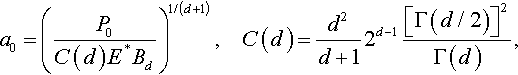
Let us consider as above axisymmetric monomial punches (Eq. 3.53) in the case of nonslipping contact conditions. If there were no surface forces, then the contact radius a0 of a punch under the external load P0 could be found from the solution given by Borodich and Keer (2004a):

The nonadhesive contact radius a1 and depth of indentation δ1 under some apparent load P1 are given by
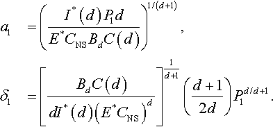
For incompressible materials, the Borodich–Keer formulae (3.167) and (3.168) are identical to the corresponding formulae of the Galin solution (3.154) and (3.155) because for ν = 0.5, one has I*(d) = 1/d and CNS = 1.
Applying the techniques descried above, one can obtain an exact formula giving the relation between the load P and the radius of the contact region a:
As in the frictionless problem above, the real displacement of the punch is δ2 = (δ1 − Δδ), i.e.,

It is convenient to write the formula for the real displacement δ2 in the case of the nonslipping boundary condition as
5.5 Universal Relations for Non-ideal-Shaped Indenters
Let us apply the results obtained above to problems of nanoindentation when the indenter shape near the tip has some deviation from its nominal shape. It is known (Borodich, 2011; Borodich et al., 2003) that at shallow depth indenter blunt shapes may often be described by homogeneous functions hd of degree d with 1 ≤ d ≤ 2. It is assumed that the indenter shape function can be approximated by a monomial function of the radius.
5.5.1 Frictionless Adhesive Indentation
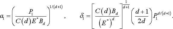
It follows from Eq. (3.156) that the radius a1 of the contact region at P0 = 0 is
As is known, the choice of the characteristic parameters of the adhesive contact problem is rather arbitrary (Borodich & Galanov, 2008). The above value of the radius can be used as a characteristic size of the contact region in order to write dimensionless parameters.
Let us write the characteristic parameters of the adhesive contact problems as

Then Eqs. (3.156) and (3.157) have the following forms:
and

5.5.2 Nonslipping Adhesive Indentation
In this case, the radius a1 of the contact region at P0 = 0 can be obtained from Eqs. (3.169):
Let us write the characteristic parameters of the nonslipping adhesive contact problems as
One can see that Eqs. (3.169) and (3.170) will have the same dimensionless form as the frictionless case. Hence, Eqs. (3.172) and (3.173) are also valid for the nonslipping adhesive JKR contact case.
5.5.3 Dimensionless Relations for Adhesive Indentation
Let us denote ![]() ,
, ![]() , and
, and ![]() . Then Eqs. (3.172) and (3.173) can be written as the following universal dimensionless relations:
. Then Eqs. (3.172) and (3.173) can be written as the following universal dimensionless relations:
and
which are valid for an arbitrary axisymmetric monomial punch of degree d ≥ 1 regardless of the contact boundary conditions (the frictionless or nonslipping conditions).
The graphs of the dimensionless relations (3.175) and (3.176) for several values of degree d of the indenter shape monomials are shown in Figs 3.7 and 3.8, respectively.


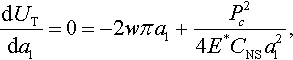
The instability point of a ![]() curve is at the point where
curve is at the point where ![]() . Taking into account that
. Taking into account that ![]() , one obtains from Eq. (3.175) at the instability point
, one obtains from Eq. (3.175) at the instability point
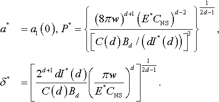
Solving this equation, one obtains for a dimensionless critical contact radius
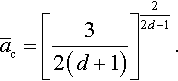
Substituting this expression into Eq. (3.175), one obtains the explicit dimensionless expression for the critical load ![]() (the adhesive force at fixed load)
(the adhesive force at fixed load)
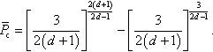
It follows from Eqs. (3.171) and (3.174) that the dimensional force of adhesion Pc does not depend on the elastic modulus of the material only if d = 2.
One can compare the critical frictionless loads PFLc with the classic solutions. Because Cd(2) = 8/3, ![]() , and (P*)FL = 6πwR for d = 2, one obtains
, and (P*)FL = 6πwR for d = 2, one obtains
This is in agreement with Eqs. (3.126) and (3.139).
One can also compare the critical loads for frictionless (PFLc) and nonslipping (PNSc) cases. Taking into account that ![]() , where (P*)FL is given by Eq. (3.171), and
, where (P*)FL is given by Eq. (3.171), and ![]() , where (P*)NS is given by Eq. (3.174), one obtains
, where (P*)NS is given by Eq. (3.174), one obtains

For frictionless (aFLc) and nonslipping (aNSc) cases, one has
