
5.5.4 Adhesive Contact for Nanoindenters of Monomial Shape
The graphs of the dimensionless ![]() relation for monomial indenters whose degree d is within the 1 ≤ d ≤ 2 range are shown in Fig. 3.9. The limiting cases of this range are conical and spherical indenters. Using the above general solution for monomial punches, one can consider analytically these limiting cases.
relation for monomial indenters whose degree d is within the 1 ≤ d ≤ 2 range are shown in Fig. 3.9. The limiting cases of this range are conical and spherical indenters. Using the above general solution for monomial punches, one can consider analytically these limiting cases.

Spherical punch. For a sphere of radius R, one has d = 2, f(r) = B2r2, B2 = 1/(2R), and C(2) = 8/3. Expression (3.156) coincides with the classic JKR formula (3.137). Further, one has ![]() . In dimensional form, one obtains the classic JKR value Pc = −(1/4)P* = −(3/2)π Rw because P* = 6π Rw for a spherical punch.
. In dimensional form, one obtains the classic JKR value Pc = −(1/4)P* = −(3/2)π Rw because P* = 6π Rw for a spherical punch.
Using Eq. (3.179) for d = 2, one can obtain the nonslipping case from the above one: PNSc = 2I*(2)PFLc.
Spence (1968) suggested using a decomposition of the integral I*(2) into a series. Using this decomposition, one obtains
For ν = 0, one has
Hence, the frictionless JKR model slightly overestimates the adhesive force for a sphere.
Conical punch (see Fig. 3.10). In the case of a cone f(r) = B1r of semi-vertical angle α, d = 1, B1 = cot α, and C(1) = π/2. It follows from Eqs. (3.177) and (3.178) that the dimensionless critical contact radius and the adhesive force at fixed load are ![]() and
and ![]() , respectively.
, respectively.

One can get the dimensional form in the frictionless case from Eq. (3.171). This gives the following values:
This is in agreement with the results obtained by Galanov (1993) and Maugis (2000).
The contact radius and displacement under zero load are, respectively,
These expressions coincide with the formulae presented by Maugis, except that formula (4.253) for δ2(0) in the book by Maugis (2000) has a wrong coefficient, 24 (see also a discussion by Borodich, Galanov, Prostov, & Suarez-Alvarez, 2012).
In the nonslipping case, one can get the dimensional form from Eq. (3.174). This gives the following values:

This is in agreement with the results obtained by Borodich, Galanov, Prostov, and Suarez-Alvarez (2012).
As has been shown (see Eq. 3.75) in this case the parameter I*(d) can be calculated exactly (Borodich & Keer, 2004a, 2004b; Spence, 1968). Hence, one obtains
The contact radius and displacement under zero load are, respectively,

Using Eq. (3.179), one obtains in the case d = 1

For ν = 0.5, one has
and hence, as expected, Eq. (3.182) coincides with Eq. (3.181). Correspondingly, for ν = 0, one has
Using Eq. (3.180), one obtains in the case d = 1

For ν = 0, one has

Thus, for compressible materials, the critical radius of the contact region and the corresponding critical load in the case of nonslipping contact are less than the predictions from the frictionless JKR approach.
6 Experimental evaluation of work of adhesion
6.1 Customary Techniques
The work of adhesion is the crucial material parameter for application of theories of adhesive contact. However, it is rather difficult to determine experimentally the values of the work of adhesion for contacting solids and, therefore, w is not a well-known quantity for many modern materials (Beach, Tormoen, Drelich, & Han, 2002).
Some concepts of fluid mechanics are often used in the mechanics of adhesion. In fluid mechanics, surface tension γ is defined as the work required to create a new liquid surface of unit area (because liquids tend to minimize their surface, this work has to be expended to increase the surface). On the other hand, as follows from the definition of w (see, e.g., Harkins, 1919), the work of cohesion is equal to the energy to pull the two identical ideal surfaces completely apart, i.e., to create a new surface; hence, w = 2γ for a liquid. Because surface energy is usually defined as the work that is required to create a new surface of unit area, the surface tension of a liquid is equal to its surface energy. The Dupré expression for the work of adhesion of two contacting liquids is w = γ1 + γ2 − γ12, where γ1, γ2, and γ12 are the surface tensions of the liquids and the interfacial tension at the interface between the liquids, respectively.
With use of the above concepts, various methods were introduced to determine the surface energy of solids. For example, to determine the surface energy of polymers it was proposed to measure the contact angle for several liquids and to employ the Young-Dupré equation and the Dupré expression (see, e.g., Owens & Wendt, 1969). However, these equations were derived for liquids, but it is known ifthe breach of adhesive connection between solids, as a rule, occurs in a nonequilibrium way and the techniques based on the transfer of these equations to solids are rather questionable (Deryagin et al., 1978).
Other techniques are based on the use of surface force apparatus (SFA). Derjaguin, Titijevskaia, Abrikossova, and Malkina (1954) published a description of the first SFA, consisting of a hemisphere and a surface of polished quartz. The hemisphere and the surface could be brought into close proximity, which could be measured by interferometry, while the force was measured by an elaborate feedback mechanism. A modified SFA was produced by Israelachvili and Tabor (1972). The modified SFA was used by Merrill, Pocius, Thakker, and Tirrell (1991) for direct measurement of molecular-level adhesive forces between biaxially oriented solid polymer films.
The AFM is used for noncontact and contact tests for evaluation of adhesive and elastic properties of materials (Cappella & Dietler, 1999). Noncontact methods of extraction of adhesive properties of polymers and other materials were discussed by Mazzola, Sebastiani, Bemporad, and Carassiti (2012). Another approach to study adhesive properties is to use a depth-sensing nanoindenter under oscillatory loading conditions (Wahl et al., 2006).
Currently, the work of adhesion is usually determined using the direct methods. Both DSI and AFM techniques can be employed. The methods differ depending on the device and the theory used. The most popular approach for estimation of the work of adhesion is based on the direct experimental measurement of the adhesive force Padh (the pull-off force) between a sphere of radius R and an elastic half-space, and the use of the JKR model. Assuming that the surfaces of the tested sample and the probe are ideally smooth, and applying directly the JKR model, one obtains Padh = PJKR, and therefore

Various approaches based on this idea were discussed by Wahl et al. (2006) and Ebenstein, Wahl (2006). It is important to realize that the Padh values obtained by direct measurements are normally poorly reproducible because the tensile (adhesive) part of the load-displacement diagram may be greatly influenced by surface roughness and the spring stiffness of the measuring device. Hence, one needs to have an extended number of experimental measurements to estimate w properly using Eq. (3.183) or using a similar method based on direct measurement of the adhesive force.
Although nanoindentation techniques may be used to study adhesive interactions of soft materials like polymers, e.g., the techniques were used by Cao, Yang, and Soboyejoy (2005) for determining the adhesion characteristics of soft polydimethylsiloxane, more often AFM techniques are used to study these interactions (see, e.g., Notbohm, Poon, & Ravichandran, 2012).
Notbohm et al. (2012) did not use Eq. (3.183), but rather they tried to find the best fit to experimental points by a shifted JKR curve. The experiments were conducted by attaching spherical particles of known radius (e.g., glass spheres with R = 5 μm) to the AFM cantilever. Then a direct least-squares error-fitting algorithm was applied to the force-displacement curve obtained for polydimethylsiloxane samples. However, it was argued earlier by Borodich, Galanov, Gorb, and Prostov (2011) that the application of the direct least-square fitting procedure to fit the data by a JKR curve does not give good results, and they suggested using the BG method. Indeed, Notbohm et al. (2012) noted that the data recorded during unloading of the AFM cantilever from the polymer specimen did not fit the JKR model.
It is known that normally Pc = Padh is less than the theoretical PJKR value because the jump out of contact occurs earlier owing to the influence of the surface roughness. This is the reason that usually one needs to have an extended number of experimental measurements to obtain the experimental value of Padh as close as possible to the true theoretical value PJKR.
Even if one assumes that Padh = PJKR, however, the force measurements are contaminated by some noise ΔP, i.e.,
and then the same error ΔP/PJKR will be transferred to ![]() . Indeed, it follows from Eq. (3.183) that
. Indeed, it follows from Eq. (3.183) that
where w is the exact value of the work of adhesion. Finally, one cannot apply the direct approach based on formula (3.183) to a truncated JKR curve, while the BG method can be applied to a truncated experimental P-δ curve.
6.2 The BG Method
6.2.1 The Basic Ideas of the Method
Borodich and Galanov (2008) introduced a method (that is called the BG method) that is not based on measurement of just one (the adhesive force) or several values of the experimental P-δ curves but it based on an inverse analysis of all experimental points at a bounded interval of the force-distance curve (the functional expression 3.143) obtained for a spherical indenter. The BG method is not direct because instead of direct measurement of the pull-off force, it needs to find some scaling parameters, and then the pull-off force is calculated using these parameters. One can expect that the compressive parts of both the loading branch and the unloading branch of the adhesive P-δ curve are not sensitive to small surface roughness. Therefore, the classic models of adhesive contact derived for smooth spheres are applicable.
The BG method reduces the problem to finding the scale characteristics Pc and δc using only the experimental points of the chosen part of the truncated force-displacement curve, e.g., the stable compressive part of the unloading branch of the P-δ curve. If (Pi, δi), i = 1,…, N are, respectively, the experimental values of the compressing load P ≥ 0 and the corresponding values of the displacement δ ≥ 0, then there is the following system of nonlinear equations for estimation of the two unknown values Pc and δc:

The above problem is ill posed according to Hadamard’s definition because the system (3.185) is overdetermined for N > 2. Hence, it is possible for such a nonlinear ill-posed problem that there exists no solution in the classic sense, and one needs to find the normal pseudosolution of the nonlinear ill-posed problem for a given set of constraints. If Pc and δc have been found, then using Eqs. (3.139) and (3.140), one can obtain the sought characteristics w and E*:

Further, one can extend the BG method to all materials having rotational symmetry of their elastic properties. In this case, one needs just to change the latter of equations (Eq. 3.186) to
6.2.2 The Robustness of the BG Method
It has been shown recently by Borodich, Galanov, Gorb, et al. (2012a, 2012b); Borodich et al. (2013) that if the origin of the displacement coordinate is known, then the BG method is very robust.
Let us consider the following numerical algorithm for checking the robustness of the BG method in application to the problem of adhesive indentation of an isotropic elastic material. The algorithm can be described as follows:
1. prescribe E* and w of a material and R of an indenter;
2. calculate Pc and δc by Eqs. (3.139) and (3.140);
3. plot the P-δ graph for these Pc and δc according to an appropriate classic model (JKR (Eq. 3.145) or DMT (Eq. 3.144));
4. take part of the P-δ graph and add to it some Gaussian noise;
5. take only the compressive part of the disturbed data;
6. solving the overdetermined problem, calculate the estimations ![]() and
and ![]() ;
;
7. calculate estimations ![]() and
and ![]() by Eq. (3.186);
by Eq. (3.186);
8. compare the initial values E* and w and their estimations ![]() and
and ![]() , and calculate the error of the BG method.
, and calculate the error of the BG method.
The application of the BG method shows that the estimations obtained for the elastic modulus and the work of adhesion have very small error even for rather contaminated data.
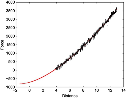
For a sphere of radius R = 3 mm and a material with the given values w = 5.66 · 10−2 N/m and E* = 1.218 MPa, the corresponding scaling parameters of the problem are, respectively, Pc = 800 μN and δc = 3.0 μm. The results obtained using the BG method from data (N = 500) for a corresponding truncated JKR curve whose compressive part is contaminated by normally distributed noise 10% of Pc and 0.1% of δc (Fig. 3.11) are ![]() ,
, ![]() ,
, ![]() , and
, and ![]() , i.e., the errors are 6.5% for w and 1.4% for E*. The units for displacements and force in Fig. 3.11 are micrometer and micronewton, respectively.
, i.e., the errors are 6.5% for w and 1.4% for E*. The units for displacements and force in Fig. 3.11 are micrometer and micronewton, respectively.
For a disturbance of 5% of both Pc and δc, the estimations are ![]() ,
, ![]() ,
, ![]() , and
, and ![]() , i.e., the errors are 3% for w and 0.6% for E*. Hence, the method is not only fast but it is also robust. The errors of the above estimations
, i.e., the errors are 3% for w and 0.6% for E*. Hence, the method is not only fast but it is also robust. The errors of the above estimations ![]() are less than the errors (Eq. 3.184) of the direct method.
are less than the errors (Eq. 3.184) of the direct method.
6.3 Application of the BG Method to Some Experimental Data
6.3.1 The Shift of the Coordinate Origin
To fit the experimental load-displacement curve, one needs to use not only the parameters Pc and δc but also an additional parameter. This is the shift of the origin of the displacement coordinate (δs). The origin of the displacement coordinate in the framework of the JKR theory is not readily extracted from the experiments. On the other hand, this reference point is very important because the solution of the overdetermined problem (3.185) is quite sensitive to the shifting of the δ values. For the JKR theory, as follows from Eq. (3.145), P(0) = −(8/9)PJKR for δ = 0, where PJKR is the theoretical value of the adhesive force.
Let us consider a coordinate system O′δ′P that can be chosen arbitrary with respect to the displacement of the coordinate origin. This means that the origin is shifted by some value δs with respect to the true coordinate system OδP that was used to derive the JKR equation. If δs > 0, then the JKR curve is located on the right from O′, and if δs < 0, then the JKR curve islocated on the left from O′. If δ′ = δs, then the point (δs, −(8/9)Pc) belongs to the JKR curve. For δs > δc, the origin O′ is taken at a point where P = 0. In this case the system (3.145) can be written as

where δ = δ′ − δs. It follows from Eq. (3.188) that the overdetermined system instead of Eq. (3.185) is written as (i = 1, 2,…, N, N > 3)

The condition N > 3 has been added because there are three unknowns: Pc, δc, and δs.
6.3.2 The Experimental Procedure
Polyvinylsiloxane (PVS) was used for experimental studies by Borodich, Galanov, Gorb, et al. (2012a, 2012b); Borodich et al. (2013). PVS is a silicone elastomer that is often used in dentistry as an impression material. The physical properties of PVSs can be modulated by variation of fillers, in particular, they can have various viscosities. The specimens were prepared in a similar way to the fibrillar specimens tested by Jiao et al. (2000). They were produced at room temperature by pouring two-compound polymerizing PVS into a smooth template lying on a smooth glass support. After the polymerization, a cast of the smooth glass was obtained. Two PVS samples were used in the experiments: the first sample had the surface as it was produced after preparation (the fresh sample), while the second surface was washed to remove possible contamination and the oxides (the washed sample).
The forces and displacements of a smooth spherical probe contacting a flat polymer surface were continuously measured. As can be seen in Fig. 3.12, the loading and unloading branches are very close to each other, and hence the contribution of viscosity to the P-δ curve of the tested samples was very low. The BG method was applied to experiments that used relatively large sapphire spheres, the radii of which were R = 1 mm and R = 3 mm, respectively. Since the surface asperities are squashed during loading, only unloading branches were studied, where the classic models of smooth adhesive contact are applicable.

The displacement of the sphere attached to a glass cantilever beam with known spring constant was detected by a fiber-optic sensor. The interacting force between the sphere and the sample was recorded as a force versus time curve. One can find a detailed description of the force tester (Tetra, Ilmenau, Germany) used in Jiao et al. (2000). All experiments were carried out at room temperature (22-24 °C) and at a relative humidity of 47-56 %. An accuracy of about 10 μN was achieved for force measurements. The spring constant was determined with an accuracy of approximately ±2.5 N/m. The spring constant of the beam with the attached sphere of R = 1 mm was k = 147 N/m, and the spring constant of the beam with the attached sphere of R = 3 mm was k = 109 N/m. Since the sphere was attached to the end of the cantilever beam, the real displacement δ of the contacting sphere is
where PΣ and δΣ are the recorded force and displacement, respectively, and δ = δΣ after the jump out of the contact point. However, the points after the jump out of the contact point were not used. Hence, δ = δΣ − PΣ/k versus PΣ graphs are presented in Fig. 3.12. Since our results show that they are quite stable, the least-squares method may be applied (Tarantola, 2004). This method enhanced by statistical filtration was used for solving overdetermined problems.
6.3.3 The Results
The results obtained for the fresh PVS sample loaded by the sphere with R = 1 mm are given in Table 3.3.
Table 3.3
The Extracted Results for the Fresh Sample Tested Using the Sphere with R = 1 mm
| Test no. | R (mm) | E* (MPa) | w · 102(J/m2) |
| 1 | 1 | 2.150 | 5.469 |
| 2 | 1 | 2.099 | 5.217 |
| 3 | 1 | 2.161 | 7.068 |
| 4 | 1 | 2.452 | 5.250 |
| 5 | 1 | 2.296 | 5.366 |
| 6 | 1 | 2.496 | 5.368 |

Hence, one obtains the following average values < E >f = 2.276 MPa and < w >f = 56.23 mJ/m2. Here and henceforth < · > denotes the average value of a parameter, and the indexes ·f and ·w mean that the value is related to the fresh or the washed sample respectively.
For the washed PVS sample loaded by the sphere with R = 1 mm, the average values of the contact modulus and the work of adhesion are < E* >w = 2.500 MPa and < w >w = 58.89 mJ/m2, respectively. The average values for both the washed sample and the fresh sample are < E* > = (2.276 + 2.500)/2 = 2.388 MPa and < w >= 55.76 mJ/m2. These results show that the elastic contact modulus and the work of adhesion of polymer materials can be reliably extracted using the enhanced statistical approach (Borodich, Galanov, Gorb, et al., 2012b; Borodich et al., 2013).
The results of application of the BG method with k = 109 J/m2 for the fresh PVS sample loaded by the sphere with R = 3 mm are as follows. The average values of the contact modulus and the work of adhesion are < E* >f = 2.38967 MPa and < w >f = 54.31 mJ/m2. For the washed sample, the average values of the contact modulus and the work of adhesion are < E* >w = 2.37683 MPa and < w >w = 60.987 mJ/m2. The average values for both the washed sample and the fresh sample are < E* > = (2.38967 + 2.37683)/2 = 2.38325 MPa and < w >= 57.6485 mJ/m2.
One can also see that washing of the sample does not affect the contact properties of the material. Indeed, it is easy to see that the error (< E* >f − < E* >)/< E* > is less than 0.3%. Although the extracted values of the contact modulus range from 2.099 to 2.925 MPa, the average values are very stable. Indeed, from experiments with R = 1 mm, it was found that < E* > = 2.388 MPa, while it follows from experiments with R = 3 mm that < E* > = 2.383 MPa. The average values of the work of adhesion vary more significantly, namely, from < w > = 55.76 mJ/m2 for R = 1 mm to < w > = 57.6485 mJ/m2 for R = 3 mm. Hence, both the instantaneous contact modulus and the work of adhesion of polymers may be treated as a material parameter only in a statistical sense.
After extracting the values sought, one needs to check whether the JKR model or the DMT models is applicable. Calculating the Tabor–Maugis parameter (Eq. 3.141), one can easily check that for all experiments μ ![]() 1, and hence the values were in the range of applicability of the JKR model.
1, and hence the values were in the range of applicability of the JKR model.
7 Concluding remarks
7.1 The Incompatibility of Adhesive Contact Problems
We have already discussed incompatibility of frictionless Hertz-type contact problems. The same types of incompatibility exist in the nonslipping contact problem (see, e.g., Spence, 1968; Zhupanska, 2009). As we have seen above, the boundary conditions of an axisymmetric self-similar Hertz-type contact problem in the Mossakovskii–Spence formulation prescribe a priori the radial and normal displacement distributions within the contact region:
These conditions may be treated as a parametric representation of the indent surface after contact of the punch and the half-space. One can show that if C0 < 0, then the punch cannot be put in the indent because it is too small; and if C0 > 0, then the indent is too large and there is no contact. Hence, the correct solution of the contact problem with boundary conditions (3.190) gives such stress fields that when applied to the boundary of an elastic half-space, produce the above-mentioned incompatibility.
Further, one has to realize that the formulation of the contact problem with nonslipping boundary conditions may lead to stress fields having oscillations near the edge of the contact region. Indeed, as shown by Abramov (1937) (see also Muskhelishvili, 1949; Rvachev & Protsenko, 1977) for the 2D problem of a nonslipping contact between a flat-ended punch of width 2l loaded by the force P, the normal p and tangential τ stress distributions are

Hence, when the coordinate x approaches the edges of the contact zone, both the normal stress and the tangential stresses change sign infinitely many times and there are tensile normal stresses within the contact region. In the axisymmetric contact problems, the displacement incompatibility is of the same type. One can see from a complete analytical solution for a nonslipping contact problem between a flat circular centrally loaded punch and an isotropic elastic half-space presented by Fabrikant (1991) that the field of radial displacements has a jump near the edge of the contact region (Fabrikant, 1991, fig. 5.1.1) and after the deformation the material points at the edge have to penetrate the punch. Evidently, this has no physical meaning. Discussing the Abramov contact problem, Muskhelishvili (1949) noted for all real solids 1 < 3 − 4ν < 3, and hence the first value |x| such that p(x) = 0 is x = ±0.9997l. Because such oscillations have no physical meaning, Rvachev and Protsenko (1977) referred to the corresponding strains as fictitious strains. They advised not to attach too much importance to the investigation of the behavior of the solutions within very small regions at singular points, where the solution may be devoid of any physical meaning (see also a recent discussion by Guo et al., 2011).
It was shown by Galanov (1993) and Galanov, Krivonos (1984a) that the problem formulation with condition (3.22) or (3.23) reduces the degree of the displacement incompatibility. However, ifone compares these solutions with the relations of the Hertz contact problem, then one can see that the influence of the refinement is rather small. Hence, the use of the JKR approach based on the use of the classic Hertz contact relations is acceptable for the adhesive contact problems considered above. Of course, this does not mean that there is no sense in studying adhesive contact using the improved problem formulations.
7.2 The Fracture Mechanics Approach to Adhesive Contact
It is known that the formulations of boundary value problems for contact mechanics are quite similar to the formulations used in fracture mechanics. In addition, the stress field near a sharp notch or a crack is singular (Wieghardt, 1907), and there is also the singular stress field at the edge of the contact region of a flat-ended punch (Boussinesq, 1885). Hence, one can try to use an asymptotic analysis of the singular stress field near the edge of the contact region in a similar way to analysis in linear fracture mechanics. The analysis presented by Maugis and Barquins (1978) showed that the results of the frictionless JKR theory can be obtained by the use of linear fracture mechanics concepts. A detailed description of the approach was presented by Maugis (2000). He showed that the singular parts of the normal stress σ33 within the contact region and the normal displacement u3 of the surface points outside the contact region at the edge of the region can be asymptotically represented using the stress intensity factor KI of the normal mode of a crack. Then, using the classic relation between the energy release rate G and KI: G = K2I/E* and applying the equilibrium equation saying that G is equal to the work of adhesion w, he derived an expression connecting two of three variables a, δ, and P in Eq. (3.128). This approach allows the researcher to draw the equilibrium curves a(P), δ(a), and P(δ). Many researchers have found that the fracture mechanics approach is very convenient for solving problems of adhesion (see, e.g., Johnson, 1996, 1997; Shull, 2002).
Thus, the results of the frictionless JKR theory can be obtained by applying the principles of linear fracture mechanics of brittle solids. However, as mentioned by Maugis (1992, 2000), this approach does not allow researchers to derive the DMT theory. Inspired by the idea of Dugdale, who represented a rather complex stress field in the vicinity of a crack tip just by a simple step function, Maugis (1992) assumed that the adhesive forces within an annulus of width ∇ outside the contact area are constant, and he obtained a transition between the JKR and DMT models of contact. The calculations were based on the idea (see, e.g., Barenblatt, 1962) that a superposition of the stress fields leads to the cancellation of the singularity term, i.e., there is no stress singularity after addition of two stress intensity factors: one due to external loading alone (the Hertz stresses are superimposed on the Boussinesq singular stresses) and the other due to external stresses acting within the annulus of width ∇.
Maugis (1992, 2000) referred to his model as based on the Dugdale fracture mechanics model. In fact, Dugdale (1960) published a brilliant engineering paper where he explained a very complicated phenomenon of cracking in an elastic-ideally plastic material just in five pages and one formula. Assuming there is a narrow strip of a plastic flow in the front of a crack, i.e., the tensile stresses in the strip are constant and equal to the yielding stress, he calculated the length of the strip such that the stresses in the solid are nonsingular. Although this model is quite inspiring, it is difficult to accept that the calculations of Dugdale (1960) (or more precisely the lack of the calculations) could critically influence Maugis. In fact, what Maugis (2000, pp. 191–200) referred to as the Dugdale model is a collection of results obtained by many authors. Let us add here some points that were not reflected by Maugis (2000). The idea to introduce a characteristic distance ∇ as a parameter of the material structure was introduced in mechanics much earlier than 1960. Studying stress concentration at sharp notches, Neuber (1937) suggested considering average stresses τav,

and to use τav to estimate the strength of a body with the notch.
Even earlier the idea to study pressure, temperature, and other physical quantities as average functions over domains was introduced in mathematics. Perhaps the ideas produced by researchers of the St Petersburg Mathematical School could be useful to study the above-mentioned problems with singularities. V.A Steklov (Stekloff) introduced a special smoothing method for functions, and N.M. Gunther (Gyunter, Gunter, Gjunter) introduced functions of domains in order to study problems in mathematical physics. It is well known that S.L. Sobolev, who was a pupil of Gunther, developed the theory of generalized functions (distributions) as functionals on a set of smooth functions Soboleff (1936). Sobolev’s theory was a development of earlier ideas of Gunther to study problems in mathematical physics using functions of domains, in particular averages of the functions over an interval (see, e.g., Gunther, 1937). In fracture mechanics, the idea to introduce the process zone in front of crack was presented by Leonov and Panasyuk (1959) and Barenblatt (1959, 1962). These models interpret the material fracture toughness as related to the interactions between atomic or molecular planes. Both models remove the stress singularity by considering a cohesive process zone ahead of the crack.
The ideas of fracture mechanics were also used for adhesive contact problems in the presence of tangential stresses. For example, Johnson (1997) used the mode-mixity fracture mechanics approach to study the Cattaneo-Mindlin-type problem, when an elastic sphere subjected to a constant normal load P and a monotonically increasing tangential force T is in contact with a flat surface. We must remember that in the problems under consideration there is no external tangential force T acting on the contacting solids.
The fracture mechanics approach to nonfrictionless adhesive contact is more complicated than in the frictionless case. Indeed, owing to analogy between adhesive contact and fracture mechanics, one would expect a kind of stress oscillatory singularity similar to Eq. (3.191). In fact, it is known (see, e.g., Tvergaard, 2001) that a crack on the interface joining two solids produces an oscillating stress singularity field which can be given in terms of the two stress intensity factor components KI and KII as
where r is the distance from the tip, ![]() , and ε is the dimensionless oscillation index. The mode mixity and its effects on adhesion were studied analytically by B. Chen, Wu, and Gao (2009) and Waters and Guduru (2010) in application to the problem of adhesive contact. In these papers it was argued that the adhesion energy is not a material constant independent of the local failure mode but rather is a function of the mode mixity. We would prefer to use Johnson’s interpretation (Johnson, 1996): the work of adhesion w is a material constant, see Eq. (3.122), while the critical energy release rate Gc is given by Gc = w[1 + α(K2II/K2I)], where the parameter α can range from 0 to 1.0. Various issues related to the use of the fracture mechanics concepts in application to the mechanics of adhesive contact between isotropic elastic materials have been discussed (see, e.g., B. Chen et al., 2009; Johnson, 1996; Waters & Guduru, 2010).
, and ε is the dimensionless oscillation index. The mode mixity and its effects on adhesion were studied analytically by B. Chen, Wu, and Gao (2009) and Waters and Guduru (2010) in application to the problem of adhesive contact. In these papers it was argued that the adhesion energy is not a material constant independent of the local failure mode but rather is a function of the mode mixity. We would prefer to use Johnson’s interpretation (Johnson, 1996): the work of adhesion w is a material constant, see Eq. (3.122), while the critical energy release rate Gc is given by Gc = w[1 + α(K2II/K2I)], where the parameter α can range from 0 to 1.0. Various issues related to the use of the fracture mechanics concepts in application to the mechanics of adhesive contact between isotropic elastic materials have been discussed (see, e.g., B. Chen et al., 2009; Johnson, 1996; Waters & Guduru, 2010).
As discussed above, the Mossakovskii–Spence formulation of the non-slipping contact problem assumes the radial displacements ur are consistent with the shape of the punch. For monomial punches of degree d, the contact problem is self-similar, the radial displacements are given by the power-law expression ur = C0rd, and the constant of the frozen-in radial displacements ensures that the radial strain at any given point of the contact zone does not change when the size of the contact region increases and both the tangential and normal contact stresses are bounded. The presence of unbounded stresses in the adhesive contact problem are due to superposition of the Boussinesq–Mossakovskii stresses in the framework of the JKR approach. If one accepts the Derjaguin approximation, then the surface energy can be calculated by Eq. (3.134), and there is no need to consider the mode mixity, and the classic JKR approach is applicable even in the nonslipping case. If the Derjaguin assumptions are not accepted and/or there is friction at the edge of the contact region (Galin, 1945; Spence, 1975; Zhupanska, 2008), then the adhesive forces can work on tangential displacements and the mode-mixity effects have to be discussed; some interesting experimental results on axisymmetric adhesive contact between a punch and a polymer layer subjected to equibiaxial stretch have been presented recently by Waters, Kalow, Gao, and Guduru (2012). Kim, McMeeking, and Johnson (1998) presented a detailed discussion of the energy fluxes upon shrinkage of the contact area for a pair of spheres in adhesion. They explained the advantages of the use of the Maugis–Dugdale approach in comparison with the direct application of the Lennard-Jones potential for modeling the interaction of adhesion and friction. A review paper by Raous (2011) discussed interface models coupling friction and adhesion, where adhesion is regarded as interface damage. In spite of considerable progress in this area, it seems that it is too early to consider as obsolete the statement by Johnson (1996) that “interaction between adhesion and friction under both static and kinetic conditions is still an open question.” Perhaps simple models of discrete structured adhesive surfaces (see, e.g., Schargott, Popov, & Gorb, 2006) may give an additional impulse to study the connections between friction and adhesion from a new point of view.
7.3 Extension of the JKR Theory to the 3D Case
The first attempt to solve a 3D adhesive contact problem was presented by Derjaguin (1934b). The above-described Derjaguin approach to adhesion of two rigid axisymmetric bodies can be easily extended to the case of two rigid 3D bodies (see also a discussion by Deryagin et al., 1978). One could try to extend the JKR approach to the 3D case directly by superposition of stress fields of the Hertz-type contact problem and the Boussinesq problem for a flat-ended punch of elliptic cross section. However, this approach would not work. Contrary to the problem of vertical indentation of an isotropic linear elastic medium by an elliptic paraboloid, the contact region of the 3D adhesive contact problem does not change homothetically, and the problem is not self-similar.
It is quite simple to check that the JKR problem is not self-similar even in the axisymmetric case. Indeed, let us take the contact radius as the problem parameter. Then it follows from Eqs. (3.138) and (3.137) that if one multiplies the parameter by λ, then the force and the displacement do not change as power-law functions of λ. The JKR approach is successful for an axisymmetric punch, because the contact region for an isotropic medium is always a circle.
Johnson and Greenwood (2005) presented an extension of the classic JKR theory to the general elliptic Hertz-type contact. They used the fracture mechanics approach to the problem. It was assumed that the contact region is always an ellipse whose ratio a/b of semiaxes varies continuously as the load is varied. Further, they calculated the stress intensity factors at the points of the edge of the contact region. Since these values are not the same, it was required that the values at the ends of the major and minor axes have to be the same. An analysis of the magnitude of the nondimensional pull-off force was presented. Because the ellipse of contact varies with the load in a nonhomothetic way, the variations with load of the mean contact radius ![]() and the compression are calculated for different values of the ratio of the main curvature radii of the elliptic paraboloid.
and the compression are calculated for different values of the ratio of the main curvature radii of the elliptic paraboloid.
7.4 An Analogy with the Inverse Approach to Impact on a Fluid Surface
Note that the above-mentioned Papkovich–Neuber formulation of the frictionless Hertz-type contact problem for an isotropic elastic half-space is mathematically quite similar to the problem of blunt body impact on the free surface of an ideal incompressible fluid. The latter problem for a fluid half-space and a wedge-shaped body was studied first by Karman and Wattendorf (1929). Their boundary value formulation did not take into account the increase of the contact region owing to motion of the fluid. The problem formulation was similar to the formulation of contact between a punch and a Winkler-Fuss (or elastic spring mattress, or Winkler-Zimmerman) foundation (see, e.g., Galin, 1961, 2008; Johnson, 1985), when the contact region can be defined as the cross section of the punch on the height δ. However, Wagner (1932) gave another formulation of the problem of impact (for details, see Borodich, 1988a, 1990e; Scolan & Korobkin, 2001, 2003).
The problem of immersion of a convex body into or impact of a convex body on a half-space of an incompressible ideal fluid is reduced to a mixed initial boundary value problem for a velocity potential Φ(x, t). If one knows the potential, then the velocities of the fluid particles v and the pressure p are defined as
where ρ is the fluid density.
The potential Φ(x, t) is a harmonic function satisfying the following conditions:
In addition, there are conditions Φ(x, t) → 0 and ∂Φ(x, t)/∂xi → 0 when |x| → ∞. Here V(t) is the body velocity.
In the Wagner formulation, the points [x*1(t), x*2(t)] at the boundary of the contact region ∂G(t) are defined from the following equation:

where the function ∂Φ/∂x3 is calculated as a function at the points of the region ![]() .
.
The symmetric 2D problem of blunt body impact in the above formulation was originally solved by Wagner (1932). The axisymmetric problem was solved by Schmieden (1953) using the Abel integral techniques. Borodich (1988a, 1990e) showed that 3D problems can be self-similar and formulated the conditions of self-similarity.
The difficulty in deriving an exact solution of the impact problem is that the contact region for an elliptic paraboloid is not an ellipse, in contrast to to the Hertz contact problem. Hence, I suggested using an inverse approach to solve the self-similar 3D impact problem and developed a procedure describing the body shape such that the contact region in the Wagner impact problem is a homothetically growing ellipse. Using an analogy between the impact problem and the crack problem, I employed a harmonic function introduced by Leonov (1940) and presented an exact solution of the 3D Wagner impact problem. The solution was presented in a rather complicated form, and I was very pessimistic that solution could be developed further analytically (Borodich, 1988a). Fortunately, I was wrong in this instance. Scolan and Korobkin (2001) noted that “since the pioneering works by Wagner (1932) and then by Borodich (1988a), the inverse problem has received little attention. However, among the major advances in that domain, one may cite exact solutions of the direct Wagner problem after calculating analytical solutions from the inverse Wagner problem.” Scolan and Korobkin (2001, 2003) designed many families of shapes for which analytical solutions of the Wagner problem can be derived. In particular, they studied the case of an elliptic contact region with no restrictions on the evolution of the semiaxes of the elliptic contact line with time, i.e., they solved non-self-similar impact problems. The progress described above in solving the inverse Wagner problem gives hope that an analogous inverse approach may be possible for solving the 3D adhesive contact problem.
Acknowledgments
My interest in contact mechanics was born during a discussion of the Hertz contact problem with my teacher Askold G. Khovanskii in 1982. I am sincerely grateful to Professor A.G. Khovanskii (Moscow and Toronto) for many years of very enjoyable meetings and discussions.
In 1984 I met Professor Boris A. Galanov (Institute for Problems in Materials Science, National Academy of Sciences of Ukraine, Kiev, Ukraine). I am very grateful to him for many years of productive discussions and sharing of ideas and results.
I am very grateful to Professor John R. Willis (Cambridge) for encouragement of my studies of contact problems and for many years of very helpful discussions.
I am very grateful to Dr. Maria M. Suarez-Alvarez (Cardiff) for inspiring my activities.
I am very grateful to Professor Leon M. Keer (Northwestern University, Evanston, USA) for his advice to study applications of contact mechanics to materials science and for many years of fruitful collaboration.
Thanks are also due to Professors Irina G. Goryacheva (Moscow), H.P. (Pwt) Evans (Cardiff), Stanislav N. Gorb (Kiel), Kenneth L. Johnson (Cambridge), Kevin Kendall (Birmingham), Yuriy I. Prostov (Moscow), and many other colleagues for discussing various aspects of problems considered in this article.