
5.5 The uniformly moving special case
For the case in which the dislocation moves uniformly with constant speed v, the past history function takes the form l(t) = vt. In that case, it is possible to find an analytical solution for elastodynamic fields of dislocations, either by the equations given in Table 2.2 or by directly solving the governing equations using η(x) = x · d where d = 1/v is the slowness of the dislocation.
In the latter case, one would obtain that the transformed potentials can be written as:
Ψ(λ,z,s)=−Δu(b2−2λ2)s2b2β[∫∞0e−s(d+λ)ξdξ]e−sβz

Φ(λ,z,s)=−2Δuλs2b2[∫∞0e−s(d+λ)ξdξ]e−sαz
These expressions can be directly integrated to obtain:
Ψ(λ,z,s)=−Δu(b2−2λ2)s2b2β1s(d+λ)e−sβz
Φ(λ,z,s)=−2Δuλs2b21s(d+λ)e−sαz

Following the same procedure as described before, on would obtain the elastodynamic fields of a uniformly moving dislocation that begun its motion at t = 0. The resulting stress field components are shown in Table 2.3. It is worth noticing that, as with the general mobile contributions, the solutions presented in Table 2.3 must be added to the injection contributions.
Table 2.3
Stress Fields for the Uniformly Moving Injected Edge Dislocation
|
A=z(a4dxz2r4+a4tz2(2x4+x2z2−z4)+a2dt2x(3x4−2x2z2−5z4)−2a2t3(x4+2x2z2−z4))r6√t2−a2r2(−a2z2+d2r2−2dtx+t2)+z(4dt4x(z2−x2)+t5(3x2−z2))r6√t2−a2r2(−a2z2+d2r2−2dtx+t2) |
|
B=z(a4dx3r4−3a4tx2z2r2+a2dt2x(−5x4−2x2z2+3z4)+a2t3(3x4+6x2z2−z4))r6√t2−a2r2(−a2z2+d2r2−2dtx+t2)+z(4dt4x(x2−z2)+t5(z2−3x2))r6√t2−a2r2(−a2z2+d2r2−2dtx+t2) |
|
C=z(b4dx(x2−z2)r4+b4tz2(−5x4−4x2z2+z4)+8b2dt2x(z4−x4)+b2t3(5x4+10x2z2−3z4))r6√t2−b2r2(−b2z2+d2r2−2dtx+t2)+z(8dt4x(x2−z2)+t5(2z2−6x2))r6√t2−b2r2(−b2z2+d2r2−2dtx+t2) |
|
D=a4dx2z2r4+a4txz2(x4−x2z2−2z4)+a2dt2(x6−5x4z2−5x2z4+z6)−a2t3x(x4−5z4)r6√t2−a2r2(−a2z2+d2r2−2dtx+t2)−dt4(x4−6x2z2+z4)+t5(x3−3xz2)r6√t2−a2r2(−a2z2+d2r2−2dtx+t2) |
|
E=b4d(x4−z4)2+b4tx(−x6−7x4z2+x2z4+7z6)−4b2dt2(x6−5x4z2−5x2z4+z6)r6√t2−b2r2(−b2z2+d2r2−2dtx+t2)+4b2t3x(x4−5z4)+4dt4(x4−6x2z2+z4)−4t5(x3−3xz2)r6√t2−b2r2(−b2z2+d2r2−2dtx+t2) |
|
σxz=μ4Δuπb2[4DH(t−ar)+EH(t−br)] |
|
σxx=4Δuπb2[−(2(λ+2μ)A+2λB)H(t−ar)−2μCH(t−br)] |
|
σzz=4Δuπb2[−(2(λ+2μ)B+2λA)H(t−ar)+2μCH(t−br)] |
|
r=√x2+z2,d=1v |


6 Aspects of the implementation of the dynamic fields of dislocations
This section tackles the arduous implementation of the numerical solution for the dynamic field of a nonuniformly moving dislocation. The injection contributions (Table 2.1) and the equations for the uniformly moving injected dislocation (Table 2.3) are polynomial expressions; despite their time-dependence, their evaluation does not differ from the elastostatic solution. Unfortunately, this is not true for the mobile contributions (Table 2.1) that are expressed as the time derivative of an a priori improper integral and depend explicitly on η(x), the inverse “past history function.”
The past history function is a nonuniform displacement law denoted by x = l(t) and defined as the x position of the dislocation line at time t. Due to the mathematical derivation followed here, it has been found more convenient to use the inverse past history function, denoted η(x). The inverse past history function or, for brevity, the past history function in the following must be thought of as the function that returns the arrival time of the dislocation line at point (x, 0). The integrals of the mobile contributions (vid. Table 2.2) are performed over a spatial variable ξ which corresponds to this very position of the dislocation line in its past history. Thus, through η(ξ), at some point in space and instant in time, the elastodynamic fields given by the mobile contributions are dependent not only on the dislocation's current position (as is the case in all quasi-static approaches) but also on each past position of the dislocation. This was in fact beautifully summarized by Eshelby as dislocations are haunted by their past (Eshelby, 1949b).
6.1 The integration limits
If the elastodynamic fields of dislocations crucially depend on the past positions of the dislocation and the integration is performed over the spatial positions of the dislocation line, one must wonder whether the improper integration limits given in Table 2.2 entail a violation of causality; the ξ → ∞ upper integration limit seems to require knowledge of the dislocation line's position beyond its current one.
This is not the case. Consider the following integral extracted from Table 2.2:
I≡I(x,z,t)=2Δuπb2∫∞0H(˜t−˜ra)˜tz[˜t2(z2−3˜x2)+a2(2˜x4+˜x2z2−z4)]Ta˜r6dξ
where ˜t=t−η(ξ)![]() , ˜x=x−ξ
, ˜x=x−ξ![]() , Ta=√˜t2−a2r2
, Ta=√˜t2−a2r2![]() with ˜r2=˜x2+z2
with ˜r2=˜x2+z2![]() .
.
Notice that the integrand is multiplied by a Heaviside function, H(˜t−a˜r)![]() . This function cancels the integrand for those values of ξ that, for a given spatial point (x, z) and instant in time t, the elastodynamic perturbations cannot have reached. Therefore, here ˜t−˜ra
. This function cancels the integrand for those values of ξ that, for a given spatial point (x, z) and instant in time t, the elastodynamic perturbations cannot have reached. Therefore, here ˜t−˜ra![]() plays the role that retarded times play in electrodynamics. It follows that causality is not broken because there is no point and instant for which H(˜t−a˜r)
plays the role that retarded times play in electrodynamics. It follows that causality is not broken because there is no point and instant for which H(˜t−a˜r)![]() does not cancel before the current time.
does not cancel before the current time.
Furthermore, in the integral above one can write:
I=2Δuπb2∫ξtξ0˜tz[˜t2(z2−3˜x2)+a2(2˜x4+˜x2z2−z4)]Ta˜r6dξ

where ξ0 and ξt are such that, for each instant in time t, they cancel the retarded time. That is, ξ0, ξt are such that
t−η(ξ(0,t))−a√(t−η(ξ(0,t)))2−a2((x−ξ(0,t))2+z2)=0

It immediately follows that both ξ0 and ξt are functions of both t and (x, z). That is, if the values of I at a certain point (x, z, t) are sought, then the integration limits will change accordingly so as to cancel the retarded time—cf. Eq. (2.85). It is clear that ξ0 = 0 for all subsonic motion. As for ξt, it marks the spot the earliest radiated elastic perturbation might have reached at time t.
6.1.1 The past history function and the mobility law
Due to the explicit dependence on a past history function η(ξ) that is not generally known, a general analytic expression of the mobile contributions in Table 2.2 cannot be achieved. There are nonetheless special cases, such as that of the uniformly moving dislocation worked out in Section 5.5.
The past history function may not be known a priori. However, it is fundamentally related to the physics of the motion of a dislocation in that, to all effects, it stores its outcome. Consider a dislocation that, at a given time t0, has its line at position x = ξ0; after a time step of magnitude Δt, the current time will be t1 = t0 + Δt, and the position of the dislocation line will have been updated to some ξ1 = ξ0 + Δξ1 in the past history function.
Mathematically, ξ and t are related in no other way than through the past history function t = η(ξ) itself. Physically, however, the dislocation line at time t0 and position ξ0 will be subjected to a series of external stimuli which, irrespective of their origin, will cause the dislocation to move in such a way that at time t1 = t0 + Δt the dislocation line is found at ξ1 = ξ0 + Δξ1. The response of the dislocation to those stimuli (typically, external stress fields) is given by the dislocation's own mobility law, the forms and origin of which discussed in greater detail in Section 8.4.
Assume for instance a mobility law that requires that the dislocation moves with
vdislocation=τBd
where vdislocation is the speed of the dislocation, d is some drag coefficient, τ an applied resolved shear stress, and B the magnitude of the Burgers vector of the dislocation. Assume that, due to numerical reasons, a D3P simulation can have a time step as small as Δt at most. Provided the value of τBd![]() is known at instant t0, the mobility law requires that, throughout the next time step, the dislocation's speed be νdisloaction=τBd
is known at instant t0, the mobility law requires that, throughout the next time step, the dislocation's speed be νdisloaction=τBd![]() . In that case, the updated position of the dislocation can immediately be calculated as ξ1 = ξ0 + vdislocation Δt.
. In that case, the updated position of the dislocation can immediately be calculated as ξ1 = ξ0 + vdislocation Δt.
This process of Euler-forward integration is employed in DDP (Van der Giessen & Needleman, 1995). D3P, as an extension of DDP, employs it as well (Gurrutxaga-Lerma et al., 2013). The integration scheme provides a natural way of building up (and storing) the past history function as a discrete sequence of pairs {(ξj, tj)}, j = 0, 1, 2,… such that each pair can be obtained by applying the mobility law to the previous state.
This would lead to a discrete past history function. However, the expressions in Table 2.2 require a continuous η(ξ). In principle, one has no knowledge of the intermediate positions inside the intervals defined by the sequence of pairs (i.e., {(ξj, ξj+l), (tj, tj+1)}, j = 0, 1, 2,…), down to the exactitude of the DD method itself. In fact, it is easy to conceive, especially for small Δt, that within a time interval the dislocation the end position of the interval, ξj+1, and then back to the interval due to vibrations, etc. Nevertheless, here the following convention is adopted: the intermediate points within an integration interval {(ξj, ξj+1), (tj, tj+1)} satisfy the mobility law, with the same kinematic parameters (velocity, acceleration, etc.) as those the dislocation takes on the lower bound of the interval, (ξj, tj).
That is, if the motion at instant tj obeys a mobility law of the form7
vdislocation=τBd|t=tj
then all the pairs in the ((ξj, ξj+1), (tj, tj+1)) interval satisfy that very same mobility law, with the values of the kinematic variables (speed, acceleration, etc.) being those at t = tj.
In this convention, η(ξ) has a form such that the position of the dislocation and its temporal derivatives (velocity, acceleration, …) satisfy the mobility law. For instance, for steps of constant speed, the past history function becomes a sequence of linear segments as depicted in Fig. 2.15. Each segment would correspond to the constant velocity of dislocations in the interval that delimits it. The relative noise appearing in elastodynamic solutions such as that shown later in Fig. 2.35B is in fact affected by the smoothness of η(x). Smoother results are obtained with approximations to η(ξ) that are smooth8 at the end of each time step, even if this means that intermediate points within the intervals do not satisfy the mobility law. There are several ways the latter can be done. For instance, one could interpolate past positions using cubic splines instead of segments, ensuring the smoothness at the end points of the past history intervals. Alternatively, smaller time steps are seen to decrease the noise in the solution. Because D3P is typically used to simulate fast phenomena such as shock loading, where the representative time can be of the order of a few picoseconds up to a few nanoseconds, the time step used is usually small enough to ensure the quality of the mobile contributions.

6.2 Numerical integration schemes
The need for a numerical integration scheme for the mobile contributions is justified by the lack of a priori knowledge of η(x). Even if it were known, the integrals to solve are usually elliptic integrals of the first, second, and third kind, which are difficult to solve analytically.
For numerical integration purposes, it is most convenient to subdivide the global integration interval, (0, ξt), into the intervals of the past history function, i.e., {(ξj, ξj+1), (tj, tj+1)}, j = 0, 1, 2,…, that is,
∫ξt0=∫ξ10+∫ξ2ξ1+⋯+∫ξj+1ξj+⋯+∫ξtξt−1

where each (ξj, ξj+1) is one of the D3P integration intervals.
Subsequently, the numerical integration can be performed over each of those subintegrals
Ij=∫ξj+1ξj

where for any integral in Table 2.2 one would have
I=∫ξt0=T−1∑j=0∫ξj+1ξj
where T corresponds with ξt.
The numerical method for the solution of each of the integrals is a matter of choice; in this work an adaptive Gauss–Kronrod (P. Davis & Rabinowitz, 1984) quadrature has been used. In general, adaptive methods seem to be the most cost effective.
However, numerical integration schemes cannot be directly used over the integrals in Table 2.2 without further care. This is due to the presence of several singularities in the integrand. These singularities require the specific treatment that is described in the following section.
6.3 Integration of the stress fields in the mobile contributions
As can be observed in Table 2.2, the stress component fields in the mobile contributions are expressed as the temporal derivative of integral expressions. There are several ways to proceed. Perhaps the most immediate one would be to numerically solve the integrals and then perform a numerical differentiation upon them. This is, however, computationally expensive and, as with all numerical derivatives of numerical data, inaccurate.
In principle, the use of algorithmic differentiation (AD) would allow for the stress field components to be obtained in parallel to the displacement field components, using forward AD schemes (Griewank & Walther, 2008) to obtain the spatial derivatives of displacement. The advantages of such a method as opposed to traditional numerical differentiation schemes such as finite differences are significant: for one thing, any discretization error is prevented, and the differential is expected to be as accurate as the underlying numerical method applied (Griewank & Walther, 2008)—in this case, that of the numerical integration scheme. Nonetheless, forward AD amounts to the analytic differentiation of the integrand of the primitives, i.e., it amounts to interchanging the order of differentiation and integration in the primitives.
As argued by Markenscoff and Clifton (1981), the interchange of the order of differentiation and integration in this case is not legitimate. It would give rise to terms of the order of T−3a and T−3b that are, in principle, nonintegrable singularities. AD or a numerical differentiation scheme over the integrals in Table 2.2 would amount to such an interchange, so further considerations are required.
The way to proceed here was devised by Markenscoff and Clifton (1981). Consider for instance a troublesome term from the transverse wave component of σxz:
σxz|b=∂∂t∫∞0H(˜t−˜rb)b4(˜x4−z4)2+T2b(8˜t2˜x2z2−˜r4˜t2)r8Tbdξ

Two terms can be identified. The second one does not produce a T−3b singularity, so the order of integration and differentiation can be interchanged directly:
i1=∂∂t∫∞0H(˜t−˜rb)Tb(8˜t2˜x2z2−˜r4˜t2)˜r8dξ=∫∞0H(˜t−˜rb)(8˜x2z2−˜r4)˜r8∂∂t[Tb˜t2]dξ==∫∞0H(˜t−˜rb)˜t(8˜x2z2−˜r4)(3˜t2−2b2˜r2)˜r8Tbdξ

In turn, the first term gives rise to the Tb−3 singularity mentioned above. It can be integrated by parts (Markenscoff & Clifton, 1981) so that the resulting integral allows the interchange as well:
i2=∂∂t∫∞0H(˜t−˜rb)b4(˜x4−z4)2˜r8Tbdξ=∂∂t∫∞0H(˜t−˜rb)b4(˜x2−z2)2˜r4(b2˜x−η′(ξ)˜t)dTb==∂∂t[b4(x2−z2)2Tb0r4(b2x−η′(0)t)]H(t−rb)−∫∞0H(˜t−˜rb)∂∂t[Tb∂∂ξ[b4(˜x2−z2)2˜r4(b2˜x−η′(ξ)˜t)]]dξ==b6(x2−z2)2[tx−r2η′(0)]r4Tb0(b2x−tη′(0))2H(t−rb)−∫∞0H(˜t−˜rb)F(˜x,z,˜t)dξ

with Tb0=√t2−b2r2![]() , r=√x2+z2
, r=√x2+z2![]() and
and
F(˜x,z,˜t)=b4(˜x2−z2)˜r6TbΓ3b{˜tΓb[b2(˜x4−8˜x2z2−z4)+8˜tz2˜xη′−(˜x2−z2)˜r2η′2+˜t(˜x2−z2)˜r2η″]+T2b[8˜t˜xz2η′2−2(˜x2−z2)˜r2η′3+b2˜x(˜x2−z2)˜r2η″+η′(2b2(˜x4−4˜x2z2−z4)+˜t(˜x2−z2)˜r2)η″]}

with Γb=b2˜x−η′(ξ)˜t![]() .
.
Throughout the derivations of the elastodynamic fields above, it is assumed that the dislocation is quiescent before it begins its motion, that is, vdislocation (t = 0+) = 0, whence η′(0+) = ∞. Therefore,
∂∂t[b4(x2−z2)2Tb0r4(b2x−η′(0)t)]H(t−rb)

must vanish. A dislocation jumping from rest to some velocity would, on the other hand, have a η(0) ≠ ∞; this case is a mere mathematical subtlety bearing little physical significance.
The procedure presented above can be equally extended to the rest of terms and components of the elastic fields. The derivatives obtained in this way are collected in Table 2.4.
Table 2.4
The Mobile Contributions as They Must Be Integrated
|
σxz=μ4Δuπb2[∫∞0H(˜t−˜ra)−˜t(˜x4−6˜x2z2+z4)(3˜t2−2a2˜r2)˜r8Tadξ−a6x2z2(−tx+r2η′(0))r4Ta(a2x−tη′(0))2H(t−ar)−∫∞0H(˜t−a˜r)∂∂t[Ta∂∂ξ[a4z2˜x2˜r4(a2˜x−˜tη′(ξ))]]dξ]−μΔuπb2[∫∞0H(˜t−˜rb)4˜t(˜x4−6˜x2z2+z4)(3˜t2−2b2˜r2)˜r8Tbdξ−b4(x2−z2)2Tb0r4(b2x−η′(0)t)H(t−br)+∫∞0H(˜t−b˜r)∂∂t[Tb∂∂ξ[b4(˜x2−z2)2˜r4(b2˜x−˜tη′(ξ))]]dξ] |
|
ux,x=−Δuπb2∫∞0H(˜t−˜ra)˜t˜xz(12˜t2(−˜x2+z2)+a2(9˜x2−11z2)˜r2)˜r8Tadξ+Δuπb2∫∞0H(˜t−˜ra)∂∂x[Ta∂∂ξ[˜ta2˜x2z˜r4(a2˜x−η′(ξ)˜t)]]dξ−Δuπb2[ta2x2zr4(a2x−η′(0)t)Ta|0]Δu2πb2∫∞0H(˜t−˜rb)−2˜t˜x(3t2(˜x3−4˜x2z−˜xz2+2z3)+b2˜r2(2˜x3−9˜x2z−3˜xz2+6z3))˜r8Tbdξ+Δu2πb2∫∞0H(˜t−˜rb)∂∂z[Tb∂∂ξ[˜tb2(z4−˜x4)z˜r6(b2˜x−η′(ξ)˜t)]]dξ−Δu2πb2[b2(z4−x4)tzr6(b2x−η′(0)t)Tb|0] |
|
uz,x=−Δuπb2∫∞0H(˜t−˜ra)˜t˜xz(12˜t2(−z2+˜x2)+a2(9z2−11˜x2)˜r2)˜r8Tadξ+Δuπb2∫∞0H(˜t−˜ra)∂∂x[Ta∂∂ξ[˜ta2˜x2z˜r4(a2˜x−η′(ξ)˜t)]]dξ−Δuπb2[ta2x2zr4(a2x−η′(0)t)Ta|0]Δu2πb2∫∞0H(˜t−˜rb)−2˜t˜x(3t2(˜x3−4˜x2z−˜xz2+2z3)+b2˜r2(2˜x3−9˜x2z−3˜xz2+6z3))˜r8Tbdξ+Δu2πb2∫∞0H(˜t−˜rb)∂∂z[Tb∂∂ξ[˜tb2(z4−˜x4)z˜r6(b2˜x−η′(ξ)˜t)]]dξ−Δu2πb2[b2(z4−x4)tzr6(b2x−η′(0)t)Tb|0] |
|
uz,z=−Δuπb2∫∞0H(˜t−˜ra)˜t(3˜r4T2a+3T2a˜x4+˜r2˜x2(−24T2a+a2(−3z2+˜x2)))˜r8Tadξ+Δuπb2∫∞0H(˜t−˜ra)∂∂z[Ta∂∂ξ[˜ta2˜xz2˜r4(a2˜x−η′(ξ)˜t)]]dξ−Δuπb2[ta2xz2r4(a2x−η′(0)t)Ta|0]−Δu2πb2∫∞0H(˜t−˜rb)2˜tz2(−3˜t2(z2+2˜xz−5˜x2)+b2(3z−4˜x)(z+3˜x)˜r2)˜r8Tbdξ+Δu2πb2∫∞0H(˜t−˜rb)∂∂z[Tb∂∂ξ[˜tb2(˜x4−z4)˜x˜r6(b2˜x−η′(ξ)˜t)]]dξ−Δu2πb2[b2(˜x4−z4)t˜xr6(b2x−η′(0)t)Tb|0] |


Integration along the dislocation's path: the z = 0 special case Besides the subtleties in the order of differentiation and integration, some of the integrals in Table 2.2 present an anomalous behavior when z = 0. This is particularly important because z = 0 corresponds with the dislocation's slip plane, i.e., the direction of motion.
For example, consider the longitudinal part of σxz in Table 2.2:
I(x,z,t)=4Δub2μ∂∂t∫∞0H(˜t−˜ra)a4˜x2z2˜r4+T2a(8˜t2˜x2z2−˜r4˜t2)˜r8Tadξ
Make z = 0. The integral becomes
I(x,0,t)=4Δub2μ∂∂t∫∞0H(˜t−|˜x|a)−˜t2Ta˜x4dξ

In this integral, at any time t the integrand is singular if x = ξ. This is not problematic as long as the singularity does not fall within the integration interval [ξ = 0, ξ = ξt]. However, for any point (x, z = 0) laying ahead of the injection site (i.e., x = 0) but behind the current position of the dislocation core (i.e., x = ξt), the denominator in Eq. (2.97) cancels (i.e., ˜x=x−ξ=0![]() ) within the integration path. Hence, the integral diverges when one tries to compute current values of the elastic field in former positions of the core of the dislocation. Not giving this case a proper consideration results in large numerical instabilities that preclude a proper computation of the values of the fields obtained along the path of the dislocation.
) within the integration path. Hence, the integral diverges when one tries to compute current values of the elastic field in former positions of the core of the dislocation. Not giving this case a proper consideration results in large numerical instabilities that preclude a proper computation of the values of the fields obtained along the path of the dislocation.
Markenscoff (1980) and Markenscoff, Clifton (1981) pointed out that a divergence in Eq. (2.96) within the integration path implies an overlooked burden in its original derivation. Take Eq. (2.96). This expression, as all the rest in Table 2.2, is derived from an integral in the reciprocal Laplace space which, prior to obtaining the Cagniard form of the integral, takes the form
I=4Δub2μ∫∞0αλ2e−sη(ξ)e−s[αz−λξ]dξ
The first inverse Laplace transform (in the spatial variable) leads to
ˆi=s2πi4Δub2μ∫i∞−i∞[∫∞0αλ2e−sη(ξ)e−s[αz−λξ]dξ]esλxdλ

Once Eq. (2.99) is obtained, the derivation of the elastodynamic fields in Section 5 proceeds to interchange the order of integration from ξ to λ by invoking Fubini's theorem. This puts the integral in its Cagniard form. It is a well-known problem, however, that Fubini's theorem is pertinent only if both the integral in ξ and the integral in λ converge (A. Taylor, 1986). Equation (2.96) highlights that the latter is not true when x falls behind the dislocation line but ahead of the injection site.
As proposed by Markenscoff (1980), the integral in Eq. (2.99) can be regularized extracting the singular part of the integral (Abramowitz, 1954). The regularization relies on noting that Eq. (2.99) diverges when η(ξ) takes values in the path of ξ. However, the integrand maintains its behavior about x = ξ if η(ξ) is approximated with its first-order Taylor about x = ξ: η(x) + (x − ξ) η′(x). Hence, consider the following integral
Iextra=4Δub2μ∫∞0αλ2e−s[(η(x)−η′(x)(x−ξ))−λξ]dξ

The first Laplace inversion of this integral becomes,
ˆiextra=s2πi4Δub2μ∫i∞−i∞[∫∞0αλ2e−s[η(x)−η′(x)(x−ξ)]esλξdξ]e−sλxdλ
Clearly, the integral in Eq. (2.99) can be regularized by adding and subtracting the integral in Eq. (2.101) to it, because by subtracting the term in Eq. (2.101) from Eq. (2.99) the singularity at x = ξ is canceled at that point (i.e., η(ξ) would cancel with η(x)).
Notice that the additional term corresponds to that of a displaced uniformly moving dislocation with speed η′(x), the fields of which have been solved in Section 5.5 and can be found in Table 2.3.
Unfortunately, this solution leads to even more lengthy formulas. In the example above, the solution would be:
I(x,0,t)=4Δuπb2μ∂∂t∫∞0[−H(˜t−|˜x|a)˜tTa˜x4+H(˜t′−|˜x|a)˜t′T′a˜x4]dξ+˜t′2T′ax3(t−η(x))H(t−η(x)+xη′(x)−|x|a)

I(x,0,t)=4Δuπb2μ∫∞0[−H(˜t−|˜x|a)˜t(3˜t2−2a2˜x2)˜x4Ta+H(˜t′−|˜x|a)˜t′(3˜t′2−2a2˜x2)˜x4T′a]dξ+˜t′2T′ax3(t−η(x))H(t−η(x)+xη′(x)−|x|a)

where ˜t′=t−η(x)+˜xη′(x)![]() , T′a=√~t′2−a2˜x2
, T′a=√~t′2−a2˜x2![]() .
.
Notice that I(x, 0, t) must be differentiated in time in order to obtain the transverse part of σxz(x, 0, t); this shall be done as explained above, integrating by parts where necessary.
The z = 0 case is relevant for the σxz and uz components alone; σxx, σzz, as well as ux vanish for z = 0.
6.4 Singularities at the injection front and behind the injection front
The elastic fields of dislocations are singular (i.e., they diverge) at the dislocation core. This is a well-known feature related to the way the core is modeled in elasticity (Hirth & Lothe, 1991). Several attempts to regularize the core analytically the core have been proposed, from the Peierls–Nabarro model (Hirth & Lothe, 1991; Nabarro, 1997; Pellegrini, 2010) to gradient elasticity theory (Lazar, 2013). Despite some recent attempts to perform computer simulations of dislocation dynamics with regularized cores (Pillon, Denoual, Madec, & Pellegrini, 2006; Po, Lazar, Seif, & Ghoniem, 2014), usually dislocations dynamics methods are primarily concerned with the long-range effects of the dislocations. For the study of long-range effects, the classical, core-diverging elastic fields are exact and, in many cases, easier to handle computationally.
However, the presence of an infinity in a computer simulation is neither possible nor desirable, and simplified regularizations have been proposed to deal with them, the most typical one being imposing cutoffs about the core. In 3D dislocation dynamics, where the Peach–Koehler forces are usually directly derived from the elastic energy of dislocations (Bulatov & Cai, 2006), the cutoff is exerted over the energy landscape; this requires the additional estimation of the core energy itself. However, in DDP simulations the Peach–Koehler forces are directly obtained from the analytical expressions of the elastic fields of the dislocations, so the core is regularized through a cutoff of the stress fields about the core itself (Van der Giessen & Needleman, 1995). In either DDP or 3D-DD, the regularization typically consists of a radial cutoff around the singular core that is a few Burgers vector wide; in DDP, the stress field within the cutoff is assumed to be constant and of a value equal to that at the radius of the cutoff.
It can be argued that the same can be done in D3P simulations, and the cutoff concept further extended to deal with an additional feature that was already commented by Markenscoff (1982): the stress field components at the injection wave fronts show singularities of order 1/√t![]() as well.
as well.
6.4.1 Location of the singularities at the injection front
Sources of singularities. The presence of singularities at the injection front can be observed in both Figs. 2.21 and 2.36; these are also evident upon inspecting the equations for the injected static fields in Table 2.1: the longitudinal and transverse parts of the stress field components are multiplied, respectively, by t/√t2−a2r2![]() and t/√t2−b2r2
and t/√t2−b2r2![]() . When t = a · r or t = b · r each denominator cancels, rendering a singularity of order 1/√t
. When t = a · r or t = b · r each denominator cancels, rendering a singularity of order 1/√t![]() .
.
The mobile contributions display the same kind of singularities at the front, but they do not identically cancel the ones due to the injection terms. Consider for instance the normal part of the σxz component of stress in the mobile contribution in the direction of the slip plane (z = 0):
∫∞0H(˜t−|˜x|a)Ta˜t2˜x4dξ
The order of integration and differentiation can be interchanged, leading to
∫∞0H(˜t−|˜x|a)˜t(3˜t2−2a2˜x2)˜x4Tadξ

A general expression of the primitive of this integral cannot be achieved inasmuch as η(ξ) is unknown. Nevertheless, it can already be hinted that if the integrand is divided by Ta, the primitive will be multiplied by it. This can be seen in some special cases; for instance, if it is assumed that the motion is uniform, i.e., η(ξ) = ξ/v, with v constant and assumed subsonic, the primitive of Eq. (2.105) takes the form
t2√t2−a2x2(t−x/v)x3H(t−a|x|)
which has no singularity at the front, and that therefore cannot cancel the one due to the injection contribution. Other cases, such as constant acceleration (η(ξ) = a/2ξ2), give rise to elliptic integrals of the first, second, and third kind, but are premultiplied by Ta as well.
Moreover, wherever there exists the singularity of a mobile contribution, cancellation is not identical. Consider the case of the transverse part of the σxz component of an uniformly moving dislocation (η(ξ) = ξ/v) in the slip plane:
4t4+b4x4−4b2t2x2x3Tb(t−x/v)H(t−b|x|)

The corresponding injection contribution term will be
−4t4+b4x4−4b2t2x2x3tTbH(t−b|x|)

The difference is therefore
4t4+b4x4−4b2t2x2x3t(tv−x)TbH(t−b|x|)

That is, the singularity at the front remains.9
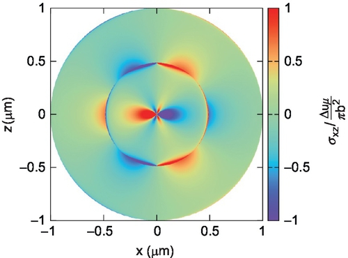
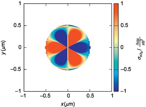
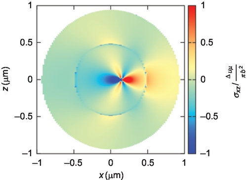
Angular dependence. There exists an angular dependency for the magnitude of the singularities at the front. Determining it is necessary if a cutoff around the singularity is to be imposed. Thus, consider for instance σzzS:
σzzs(x,z,t)=2Δuπb2tz[a2Λr4+μ[6a2x2r2+2t2(z2−3x2)]]r6√t2−r2a2H(t−ra)−2Δuμπb2tz[2t2(z2−3x2)+b2[5x4+4x2z2−z4]]r6√t2−b2r2H(t−rb)

At t = ar, the longitudinal front part is singular, the numerator being
ar2z(a2Λr4+2μa2r2z2)
In polar coordinates, z = r sin θ so that the numerator becomes
a3r6sinθ(Λ+2μsin2θ)
which means that the singularity vanishes at sin θ = 0, i.e., for θ = 0, π (the direction of the x-axis), as it can be readily observed in Fig. 2.36B. The same analysis, performed for the shear front in the same component, shows that
b3r6sinθ(sin2θ−cos2θ)
which implies that the singularity in the transverse front vanishes for θ = nπ and for θ=nπ/4(n∈Z)![]() irrespective of the elastic constant values. This feature is also observed in Fig. 2.36B.
irrespective of the elastic constant values. This feature is also observed in Fig. 2.36B.
Performing the same analysis for σxxS, it can be observed that the singularity vanishes at θ = nπ for the longitudinal front and at θ = nπ and θ=(2n+1)π/4(n∈Z)![]() in the transverse front. For σxzS, the singularity vanishes at θ = (2n + 1)π/2 for the longitudinal front and θ = (2n + 1)π/2 and θ = (2n + 1)π/4 for the transverse front. Again, these features can be readily observed in Fig. 2.36A and C, respectively, and match the observations made by Markenscoff (1982) and Markenscoff, Clifton (1981) for the front ahead of the uniformly moving edge dislocation.
in the transverse front. For σxzS, the singularity vanishes at θ = (2n + 1)π/2 for the longitudinal front and θ = (2n + 1)π/2 and θ = (2n + 1)π/4 for the transverse front. Again, these features can be readily observed in Fig. 2.36A and C, respectively, and match the observations made by Markenscoff (1982) and Markenscoff, Clifton (1981) for the front ahead of the uniformly moving edge dislocation.
Singularities behind the front. The only singularities behind the front are those at the current position of the dislocation—i.e., the current position of the core for mobile contributions alone—and the injection site—for both injection and mobile contributions. However, the latter vanishes when the injection contribution is summed with the mobile contribution.
The injection contributions do not have sources of singularities behind the front other than the aforementioned injection site. And the only additional source of singularities in the mobile contributions comes from terms such as
a2z∂∂t[xz√t2−a2(x2+z2)√x2+z2(a2x−tη′(0))]H(t−ar)

However, the a2x − tη′(0) denominator in those nonintegral terms can only produce a singularity if η′(0) ≠ ∞, which as has already been mentioned cannot occur provided the dislocation is quiescent upon injection. Even then, aside from the Ta0![]() singularity, the a2x − tη′(0) singularity can only mathematically happen ahead of the front, something that is prevented by the Heaviside function.
singularity, the a2x − tη′(0) singularity can only mathematically happen ahead of the front, something that is prevented by the Heaviside function.
Cutoffs at the singularities. As shown, there are two types of singularities: those due to the dislocation core and those due to the propagating injection fronts. As with DDP (Van der Giessen & Needleman, 1995), D3P simulations must ensure that, for numerical purposes, no infinities are present; in DDP, where the only source of infinities is the dislocation core, this is achieved by imposing a radial cutoff distance around the core, within which the stress is assumed to be constant but of a very high value, typically the same magnitude as the one predicted by elasticity at the boundary of the core.
In DDP, in order to prevent the aforementioned presence of infinities, a typical cutoff radius of about 2–10 Burgers vectors is most commonly defined (Van der Giessen & Needleman, 1995). It is proposed that D3P simulations enforce a cutoffradius of similar magnitude around the moving core.
As with the core cutoff, a safety ring needs to be established around the singular regions of the injection front. A ring about 2–10 Burgers vectors wide should suffice, with its angular distribution corresponding to that of the singularities at the front themselves, described above. It must be pointed out that the presence of singularities at the front suggests that when it encounters a dislocation, the dislocation will, for a short time, undergo an unusually large Peach–Koehler force. Under the action of such a force, the mobility law ought to prevent the dislocation from reaching unphysical velocities.
7 The moving fields of dislocations
The main qualitative feature of the dynamic solutions to the elastic fields here discussed is their wave structure. All the fields are composed of terms propagating at the longitudinal speed of sound, followed by terms propagating at the slower transverse speed of sound. This gives rise to a characteristic two-wave structure, with an outer longitudinal wave followed by an inner transverse front, both in the form of concentrical circumferences radiating outward from the dislocation core.
These features are an expression of causality. They signify that, at a given spatial point and instant in time, the effect of a dislocation is experienced only if its elastic perturbations have sufficient time to reach that location. That is to say, the dynamic fields of dislocations cause the interactions between dislocations to be based on a retardation principle. This retardation principle is further complicated by the fact that the dislocation core can move, and do so nonuniformly, in which case the effect that the dislocation's fields have on a given spatial point will vary depending on the exact nature of the perturbation that has reached it; the latter depends upon the dislocation's past history.
As a result, the dynamic fields of dislocations introduce a radical change of paradigm with respect to the DDP methodology; in previous quasi-static discrete dislocation methods, all field interactions were instantaneous. The elastodynamic extension of DDP presented here has been named “dynamic discrete dislocation plasticity” (D3P). In this section, the main features of the dynamic fields are examined, paying particular attention to how these may affect dislocation interactions.
7.1 The injection contribution term
The injection contribution refers to the creation (injection) of a quiescent straight edge dislocation. The analytical form of these fields, the derivation of which is given in Section 5, is presented in Table 2.1. The form of these fields can be seen in Figs. 2.16–2.18.


The main characteristic of these fields is their form as two concentric circles about the dislocation's core. They are the longitudinal and transverse wave perturbations arising as a result of the injection, which travel, respectively, at ct and c1. This can be clearly seen in
σxz(x,z,t)=−4Δuμπb2tx[t2(x2−3z2)+a2(2z4−x4+x2z2)]r6√t2−r2a2H(t−ra)−Δuμπb2tx[−4t4(x2−3z2)+4b2t2(x4−5z4)]r6(t2−b2z2)√t2−b2r2H(t−rb)−Δuμπb2tx[b4(7z6+x2z4−7x4z2−x6)]r6(t2−b2z2)√t2−b2r2H(t−rb)

where two clear terms, one depending on H (t − ra) and another one depending on H (t − rb), can be seen:
σxztransverse(x,z,t)=−4Δuμπb2tx[t2(x2−3z2)+a2(2z4−x4+x2z2)]r6√t2−r2a2H(t−ra)

σxzlongitudinal(x,z,t)=−Δuμπb2tx[−4t4(x2−3z2)+4b2t2(x4−5z4)]r6(t2−b2z2)√t2−b2r2H(t−rb)−Δuμπb2tx[b4(7z6+x2z4−7x4z2−x6)]r6(t2−b2z2)√t2−b2r2H(t−rb)
These two field contributions are depicted in Figs. 2.19 and 2.20. Needless to say, their summation renders Fig. 2.16. The waves are preceded by two injection fronts that display several singularities as discussed in Section 6.4.

As proven in Section 5.3, the solution inside the transverse injection front converges quickly to the traditional elastostatic solution. However, in contrast to the elastostatic “steady-state” solution, the elastodynamic fields do not exist everywhere in the domain. This is seen clearly in Fig. 2.21, which shows the temporal evolution of the σxz (x, z, t) component of stress: spreading outward from the core, the magnitude of the field in Fig. 2.21C converges to that of the elastostatic solution in Fig. 2.21D after a few nanoseconds. However, the elastostatic solution becomes recognizable only after the transverse front has passed, and causation is never violated: the fields are zero in points far away from the point of injection even if they have already converged to the elastostatic solution in points close to the point of injection.

 . The material properties of aluminum were used. (A) t = 0.05 ns. (B) t = 0.1 ns. (C) t = 0.2 ns. (D) Static solution. Image courtesy of Gurrutxaga-Lerma et al. (2013).
These dynamic features make interactions between dislocations all the more interesting, because not only they imply that the effect of dislocations is not experienced instantaneously everywhere in the medium, but that the interactions can be radically different from their elastostatic counterpart. Consider for instance a point first encountered by the longitudinal injection front. This front travels at a speed that in most metals is roughly twice as large as the transverse speed of sound, so for roughly half of the time it takes for a longitudinal perturbation emanating from the core at that precise instant in time to reach the point, the only fields the point will feel are those corresponding to the longitudinal component alone, i.e., those depicted in Fig. 2.19. The further away the point is from the point of injection, the longer it will take for the transverse front to reach it. And, as said above, the injection fields only converge to their elastostatic counterparts inside the transverse front, so for a long while the point are feeling a stress field that has little to do with the elastostatic values.
7.2 The injected uniformly moving edge dislocation
The injected uniformly moving edge dislocation refers to a dislocation that is injected at t = 0 and begins to move with a constant, uniform speed v. The analytic expressions of the fields have been derived in Section 5.5 and are presented in Table 2.2. They are a useful solution to bear in mind because, despite having the simplest of all past history functions, or precisely because of that, they serve to highlight many of the dynamic effects that nonuniformly moving dislocations display.
As with the injected, nonmoving dislocation, here the elastic fields display the characteristic two-wave structure of a longitudinal front followed by a transverse front. However, the fields themselves are affected by the motion of the core. Figure 2.22 shows the σxz stress field component of a straight edge dislocation moving with Mt = 0.3.10 As can be seen, the fields display the characteristic lobular structure also seen in Fig. 2.16, which showed the injected quiescent dislocation. Except for the fact that the dislocation's core has moved in Fig. 2.22, both solutions appear to be remarkably similar both in magnitude of the fields and shape. However, this does not justify invoking a quasi-static argument here, and using the displaced solutions for the nonmoving injected dislocation instead: in Fig. 2.22, the core is not centered about the longitudinal and transverse injection fronts, while in Fig. 2.16 it is. Notice that reversal in the sign between Figs. 2.16 and 2.22 is simply explained because Fig. 2.16 represents the injection contribution, whose sign is the inverse of the moving contribution's.
Furthermore, as it happened with the Eshelby solutions for the preexisting uniformly moving dislocation (q.v. Section 3.1), the fields tend to deform as the speed of the dislocation is increased. Figure 2.23 for instance shows the σxz stress field component at Mt = 0.77, for the same instant in time as in Fig. 2.22. As with the solutions presented in Fig. 2.7, the fields experience a contraction in the direction of motion. Here, however, this contraction overlaps with the injection fronts, causing intense stress gradients about the dislocation's core which, necessarily, is fairly close to the transverse injection front itself (the inner ring). At the same time, the horizontal lobes tend to decrease in size and magnitude, just as it happened with the Eshelby solutions. This contraction becomes exceedingly large for very high speeds; Fig. 2.24 shows the fields at Mt = 0.92, above the Rayleigh wave speed, and Fig. 2.25 at Mt = 0.9999, roughly at the sound barrier.


In these two figures, one can appreciate that the contractions occur fundamentally in the transverse component of the fields; in fact, the intensity of the horizontal lobe of the longitudinal component about the transverse injection front triples as the dislocation's speed increases. This contraction is also present in the σxx and σzz components; Figs. 2.27 and 2.29 show the contracted σxx and σyy fields, respectively, at Mt = 0.93; these contractions are not apparent at lower speeds, as shown in Figs. 2.26 and 2.28 of, respectively, the σxx and σyy components at Mt = 0.3.

7.2.1 Dynamic effects
The contraction and increase in the relative magnitude of the elastodynamic fields of dislocations moving at high speeds is a feature that cannot be captured using traditional static dislocation theory.
As can be seen from Figs. 2.22, 2.26, and 2.28 at Mt = 0.3, the magnitude of the elastodynamic fields are rather weak in the direction of motion ahead of the transverse front but behind the longitudinal one (the outer ring); for Mt = 0.93, as it can be seen in Figs. 2.24, 2.27, and 2.29, the magnitude of the fields has increased, almost doubled, in that very same location (Figs. 2.27–2.29).


These effects are equally reflected when one rotates the elastodynamic fields. Consider a dislocation moving with Mt = 0.93 on a −45° plane with respect to the global x-direction. Upon rotating the stress field components to obtain σxx for such dislocation, the fields obtained in Figs. 2.30 and 2.31 are obtained. As can be seen, the fields are much stronger in the outer ring when Mt = 0.93 (Fig. 2.31) than when Mt = 0.3 (Fig. 2.30).

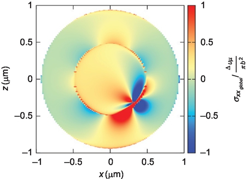
This highlights that the longitudinal components of the fields experience a dramatic increase in magnitude ahead of the core, and that this magnification is not entirely reflected on the transverse components that converge to the quasi-static solution at t → ∞ (Gurrutxaga-Lerma et al., 2013). That its partner in a dipole, moving away from the front, influences the front less because the fields behind the core are comparatively much weaker than their quasi-static counterpart when dynamic effects are accounted for. Hence, fast moving dipoles relax the medium more ahead of themselves than their elastostatic counterparts. These effects are entirely missed unless one uses a fully dynamic formulation such as D3P.