In the previous chapters, you have looked at fully connected networks and all the problems encountered while training them. The network architecture we have used, one in which each neuron in a layer is connected to all neurons in the previous and following layer, is not really good at many fundamental tasks, such as image recognition, speech recognition, time series prediction, and many more. Convolutional neural networks (CNNs) and recurrent neural networks (RNNs) are the advanced architectures most often used today. In this chapter, you will look at convolution and pooling, the basic building blocks of CNNs. Then you will check how RNNs work on a high level, and you will look at a select number of examples of applications. I will also discuss a complete, although basic, implementation of CNNs and RNNs in TensorFlow. The topic of CNNs and RNNs is much too vast to cover in a single chapter. Therefore, I will cover here only the fundamental concepts, to show you how those architectures work, but a complete treatment would require a separate book.
Kernels and Filters
One of the main components of CNNs are filters—square matrices that have dimensions nK × nK, where, usually, nK is a small number, such as 3 or 5. Sometimes, filters are also called kernels. Let’s define four different filters and check their effect later in the chapter, when they are used in convolution operations. For these examples, we will work with 3 × 3 filters. For the moment, consider the following definitions just for reference; you will see how to use them later in the chapter.
The following kernel will allow the detection of horizontal edges:
The following kernel will allow the detection of vertical edges:
The following kernel will allow the detection of edges when luminosity changes drastically:
The following kernel will blur edges in an image:
In the next sections, we will apply convolution to a test image with the filters, and you will see what its effect is.
Convolution
The first step toward understanding CNNs is to understand convolution. The easiest way to see it in action is in a few simple cases. First, in the context of neural networks, convolution is done between tensors. The operation gets two tensors as input and produces a tensor as output. The operation is usually indicated with the operator ∗. Let’s see how it works. Let’s get two tensors, both with dimensions 3 × 3. The convolution operation is performed by applying the following formula:
In this case, the result is simply the sum of each element ai, multiplied by the respective element ki. In a more typical matrix formalism, this formula could be written with a double sum as
But the first version has the advantage of making the fundamental idea very clear: each element from one tensor is multiplied by the corresponding element (the element in the same position) of the second tensor, and then all the values are summed to get the result.
In the previous section, I mentioned kernels, and the reason is that convolution is usually done between a tensor, which we may indicate here with A, and a kernel. Typically, kernels are small, 3 × 3 or 5 × 5, while the input tensors A are normally bigger. In image recognition, for example, the input tensors A are the images that may have dimensions as high as 1024 × 1024 × 3, where 1024 × 1024 is the resolution, and the last dimension (3) is the number of the color channels, the RGB (red, green, blue) values. In advanced applications, the images may have even higher resolution. How do we apply convolution when we have matrices with different dimensions? To understand how, let’s consider a matrix A that is 4 × 4.
And let’s see how to do convolution with a kernel K, which, for this example, we will take to be 3 × 3.
The idea is to start at the top-left corner of matrix A and select a 3 × 3 region. In our example, that would be
or the elements marked in boldface following.
Then we perform the convolution, as explained at the beginning, between this smaller matrix A1 and K, getting (we will indicate the result with B1)
Then we must shift the selected 3 × 3 region in matrix A by one column to the right and select the elements marked in boldface following.
That will give us the second sub-matrix A2
and we perform again the convolution between this smaller matrix A2 and K
Now we cannot shift our 3 × 3 region any more to the right, because we have reached the end of matrix A, so what we do is shift it one row down and start again from the left side. The next selected region would be
Again, we perform the convolution of A3 with K
As you may have guessed by this point, the last step is to shift our 3 × 3 selected region to the right by one column and perform the convolution again. Our selected region will now be
and the convolution will give the result
Now we cannot shift our 3 × 3 region any more, neither right nor down. We have calculated 4 values: B1, B2, B3, and B4. Those elements will form the resulting tensor of the convolution operation, giving us the tensor B.
The same process can be applied when the tensor A is bigger. You will simply get a bigger resulting B tensor, but the algorithm to get the elements Bi is the same. Before moving on, there is still a small detail that I must discuss, and that is the concept of stride. In the preceding process, we always have moved our 3 × 3 region one column to the right and one row down. The number of rows and columns, in this example 1, is called stride and is often indicated with s. Stride s = 2 means simply that we would shift our 3 × 3 region two columns to the right and two rows down. Something else that I must discuss is the size of the selected region in the input matrix A. The dimensions of the selected region that we shifted around in the process must be the same as that of the kernel used. If you use a 5 × 5 kernel, then you must select a 5 × 5 region in A. In general, given a nK × nK kernel, you will select a nK × nK region in A.
A more formal definition is that convolution with stride s, in the neural network context, is a process that takes a tensor A of dimensions nA × nA and a kernel K of dimensions nK × nK and gives as output a matrix B of dimensions nB × nB with
where we have indicated with ⌊x⌋ the integer part of x (in the programming world, this is often called the floor of x). A proof of this formula would take too long to discuss, but it is easy to see why it is true (try to derive it). To make things a bit easier, we will suppose that nK is odd. You will see soon why this is important (although not fundamental). Let me begin explaining formally the case with a stride s = 1. The algorithm generates a new tensor B from an input tensor A and a kernel K, according to the formula
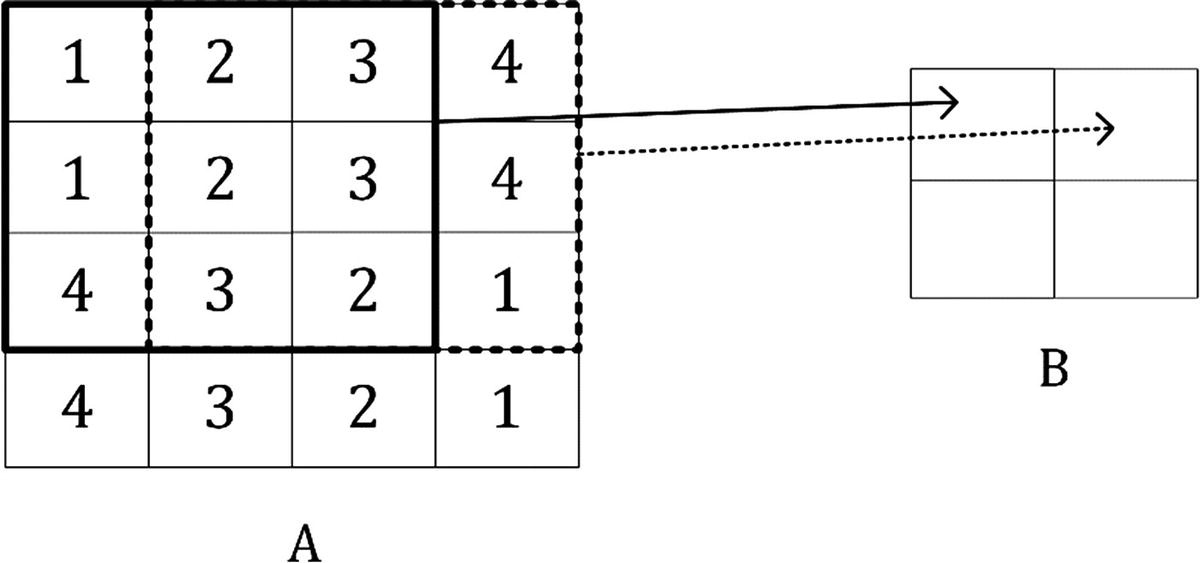
The formula is cryptic and very difficult to understand. Let’s see some more examples, to grasp the meaning better. In Figure 8-1, you can see a visual explanation of how convolution works. Suppose you have a 3 × 3 filter. Then, in the figure, you can see that the top left nine elements of the matrix A, marked by a square drawn with a black continuous line, are the ones used to generate the first element of the matrix B1, according to the preceding formula. The elements marked by the square drawn with a dotted line are the ones used to generate the second element B2, and so on. To reiterate what I discussed in the example at the beginning, the basic idea is that each element of the 3 × 3 square from matrix A is multiplied by the corresponding element of the kernel K, and all the numbers are summed. The sum is then the element of the new matrix B. After having calculated the value for B1, you shift the region you are considering in the original matrix by one column to the right (the square indicated in Figure 8-1 with a dotted line) and repeat the operation. You continue to shift your region to the right, until you reach the border, and then you move one element down and start again from the left and continue in this fashion until reaching the lower right angle of the matrix. The same kernel is used for all the regions in the original matrix.
Figure 8-1
Visual explanation of convolution
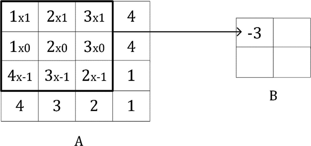
Given the kernel , for example, you can see in Figure 8-2 which element of A gets multiplied by which element in and the result for the element B1, that is nothing else as the sum of all the multiplications
Figure 8-2
Visualization of convolution with the kernel
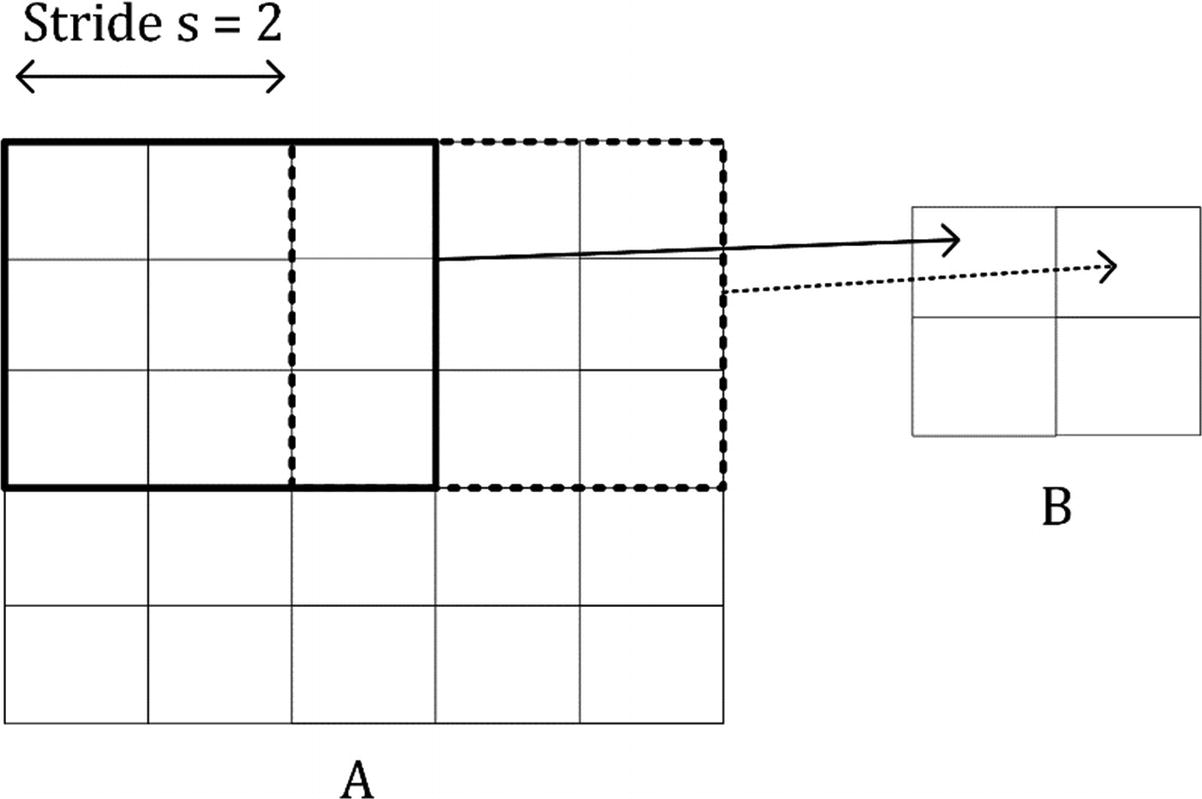
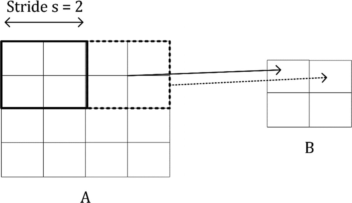
In Figure 8-3, you can see an illustrative example of convolution with stride s = 2.
Figure 8-3
Visual explanation of convolution with stride s = 2
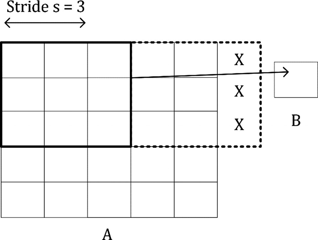
The reason why the dimension of the output matrix takes only the floor (the integer part) of can be seen intuitively in Figure 8-4. If s > 1, what can happen, depending on the dimensions of A, is that at a certain point, you cannot shift your window on matrix A (the black square in Figure 8-3, for example) anymore, and you cannot cover all of matrix A completely. In Figure 8-4, you can see how you would need an additional column on the right of matrix A (marked by many Xs), to be able to perform the convolution operation. In Figure 8-4, s = 3, and since we have nA = 5 and nK = 3, B will a scalar as a result.
Figure 8-4
Visual explanation of why the floor function is required when evaluating the resulting matrix B dimensions
You can easily see from Figure 8-4 how with a 3 × 3 region you can only cover the top-left region of A, because with stride s = 3, you would end up outside A and, therefore, could consider only one region for the convolution operation, thereby ending up with a scalar for the resulting tensor B.
Let’s now consider a few additional examples, to make this formula even clearer. Let’s start with a small matrix 3 × 3.
And let’s consider the kernel
and the stride s = 1. The convolution will be given by
and the result B will be a scalar, because nA = 3, nK = 3, therefore
If you consider now a matrix A with dimensions 4 × 4, or nA = 4, nK = 3 and s = 1, you will get as output a matrix B with dimensions 2 × 2, because
For example, you can verify that given
and
we have with stride s = 1
Let’s verify one of the elements, B11, with the formula I gave you. We have
Note that the formula I gave you for the convolution works only for stride s = 1 but can be easily generalized for other values of s.
This calculation is very easy to implement in Python. The following function can evaluate the convolution of two matrices easily enough for s = 1. (You can do it in Python with already existing functions, but I think it is instructive to see how to do it from scratch.)
Note that the input matrixA does not even need to be a square one, but it is assumed that the kernel is, and that its dimension nK is odd. The previous example can be evaluated with the following code:
A = np.array([[1,2,3,4],[5,6,7,8],[9,10,11,12],[13,14,15,16]])
K = np.array([[1,2,3],[4,5,6],[7,8,9]])
print(conv_2d(A,K))
This gives the result
[[ 348. 393.]
[ 528. 573.]]
Examples of Convolution
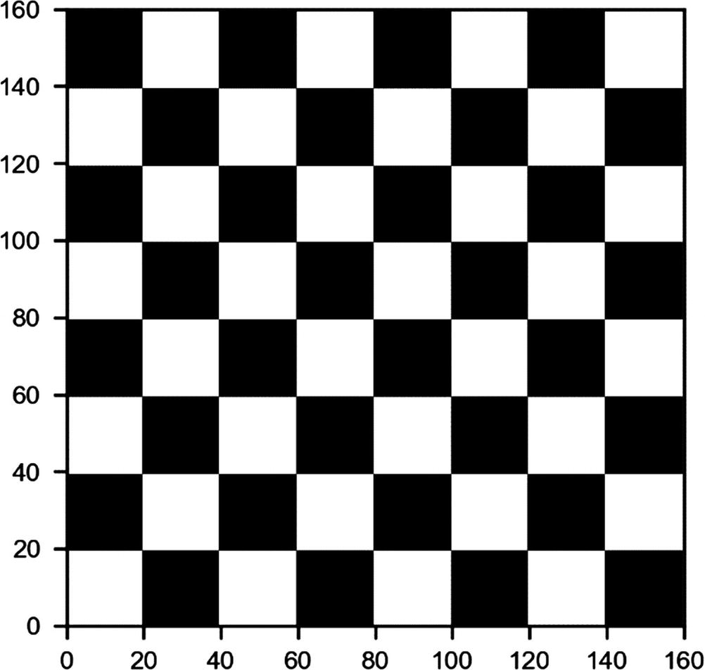
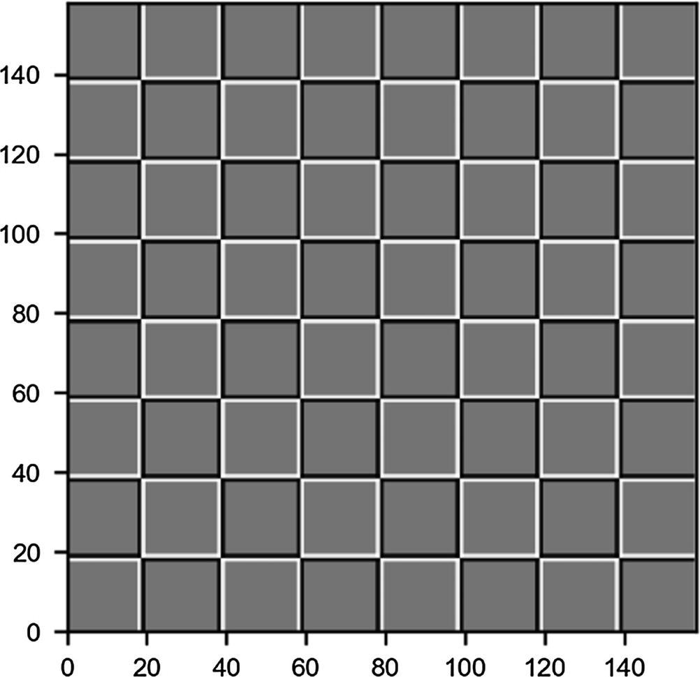
Now let’s try to apply the kernels we have defined at the beginning to a test image and see the results. As a test image, let’s create a chessboard having the dimensions 160 × 160 pixels, with the code
In Figure 8-5, you can see how the chessboard looks.
Figure 8-5
Chessboard image generated with code
Now let’s try to apply convolution to this image with the different kernels with stride s = 1.
Using the kernel will detect the horizontal edges. This can be applied with the code
edgeh = np.matrix('1 1 1; 0 0 0; -1 -1 -1')
outputh = conv_2d (chessboard, edgeh)
In Figure 8-6, you can see what the output looks like.
Figure 8-6
Result of performing a convolution between the kernel and the chessboard image
Now you can understand why I said that this kernel detects horizontal edges. Additionally, this kernel detects if you go from light to dark or vice versa. Note that this image is only 158 × 158 pixels, as expected, because
In Figure 8-9, you can see two plots: on the left, the blurred image, and on the right, the original one. The images show only a small region of the original chessboard, to make the blurring clearer.
Figure 8-9
Effect of the blurring kernel . On the left is the blurred image, and on the right, the original one.
To finish this section let’s try to understand better how the edges can be detected. Let’s consider the following matrix with a sharp vertical transition, because the left part is full of tens and the right part full of zeros.
Now let’s consider the kernel . We can perform the convolution with the code
ex_out = conv_2d (ex_mat, edgev)
The result is
array([[ 0., 0., 30., 30., 0., 0.],
[ 0., 0., 30., 30., 0., 0.],
[ 0., 0., 30., 30., 0., 0.],
[ 0., 0., 30., 30., 0., 0.],
[ 0., 0., 30., 30., 0., 0.],
[ 0., 0., 30., 30., 0., 0.]])
In Figure 8-10, you can see the original matrix (on the left) and the output of the convolution (on the right). The convolution with the kernel has clearly detected the sharp transition in the original matrix, marking with a vertical black line where the transition from black to white occurs. For example, consider B11 = 0.
Note that in the input matrix
there is no transition, as all the values are the same. On the contrary, if you consider B13, you must consider this region of the input matrix
where there is a clear transition, because the rightmost column is made up of zeros, and the rest of tens. You get now a different result.
And this is exactly how, as soon as there is a big change in values along the horizontal direction, the convolution will return a high value, because the values multiplied by the column with 1 in the kernel will be bigger. When, conversely, there is a transition from small to high values along the horizontal axis, the elements multiplied by -1 will give a result that is bigger in absolute value, and, therefore, the final result will be negative and big in absolute value. This is the reason why this kernel can also detect if you pass from a light color to a darker color or vice versa. In fact, if you consider the opposite transition (from 0 to 10) in a hypothetical different matrix A, you would have
because, this time, we move from 0 to 10 along the horizontal direction.
Figure 8-10
Result of the convolution of the matrix ex_mat with the kernel , as described in the text
Note how, as expected, the output matrix has dimensions 5 × 5, because the original matrix has dimensions 7 × 7, and the kernel is 3 × 3.
Pooling
Pooling is the second operation that is fundamental to CNNs. This operation is much easier to understand than convolution. To understand it, let’s again consider a concrete example and what is called max pooling. Let’s again use the 4 × 4 matrix from our discussion of convolution.
To perform max pooling, we must define a region of size nK × nK, analogous to what we did for convolution. Let’s consider nK = 2. What we must do is start at the top-left corner of our matrix A and select a nK × nK region, in our case, 2 × 2, from A. Here, we select
or the elements marked in boldface in matrix A, as follows:
From the elements selected, a1, a2, a5, and a6, the max pooling operation selects the maximum value, giving a result that we will indicate with B1.
Now we must shift our 2 × 2 window two columns, typically the same number of columns the selected region has, to the right and select the elements marked in boldface
or, in other words, the smaller matrix.
The max-pooling algorithm will then select the maximum of the values, giving a result that we will indicate with B2.
At this point, we cannot shift the 2 × 2 region to the right anymore, so we shift it two rows down and start the process again, from the left side of A, selecting the elements marked in boldface and getting the maximum and calling it B3, as follows:
The stride s in this context has the same meaning already covered in the discussion on convolution. It is simply the number of rows or columns you move your region when selecting the elements. Finally, we select the last region, 2 × 2, in the bottom lower part of A, selecting the elements a11, a12, a15, and a16. We then get the maximum, and we then call it B4. With the values we obtain in this process, in our example, the four values B1, B2, B3 and B4, we will build an output tensor.
In the example, we have s = 2. Basically, this operation takes as input a matrix A, a stride s, and a kernel size nK (the dimension of the region we selected in the previous example) and return a new matrix B, with dimensions given by the same formula we applied in the discussion of convolution.
To reiterate, the idea is to start from the top left of your matrix A, take a region of dimensions nK × nK, apply the max function to the selected elements, then shift the region of s elements toward the right, select a new region—again of dimensions nK × nK—apply the function to its values, and so on. In Figure 8-11, you can see how you would select the elements from a matrix A with a stride s = 2
Figure 8-11
Visualization of pooling with stride s = 2
For example, applying max pooling to the input A
will get you the result (it is very easy to verify)
because 4 is the maximum of the values marked in boldface
11 is the maximum of the values marked in boldface, as follows:
and so on. It is worth mentioning another way of doing pooling, although not as widely used as max pooling: average pooling. Instead of returning the maximum of the selected values, it returns the average.
Note
The most used pooling operation is max pooling. Average pooling is not as widely used but can be found in specific network architectures.
Padding
Worth mentioning is the concept of padding. Sometimes, when dealing with images, it is not optimal to get a result from a convolution operation that has dimensions that are different from those of the original image. So, sometimes, you do what is called padding. Basically, the idea is very simple: it consists of adding rows of pixels at the top, bottom, and columns of pixels on the right and on the left of the final images, filled with some values to make the resulting matrices the same size as the original one. Some strategies are to fill the added pixels with zeros, with the values of the closest pixels, and so on. In our example, our ex_out matrix with zero padding would look like this:
array([[ 0., 0., 0., 0., 0., 0., 0., 0.],
[ 0., 0., 0., 30., 30., 0., 0., 0.],
[ 0., 0., 0., 30., 30., 0., 0., 0.],
[ 0., 0., 0., 30., 30., 0., 0., 0.],
[ 0., 0., 0., 30., 30., 0., 0., 0.],
[ 0., 0., 0., 30., 30., 0., 0., 0.],
[ 0., 0., 0., 30., 30., 0., 0., 0.],
[ 0., 0., 0., 0., 0., 0., 0., 0.]])
The use and reasons behind padding are beyond the scope of this book, but it is important to know that it exists. Only as a reference, in case you use padding p (the width of the rows and columns you use as padding), the final dimensions of the matrix B, in case of both convolution and pooling, is given by
Note
When dealing with real images, you always code color images in three channels: RGB. This means that you must execute convolution and pooling in three dimensions: width, height, and color channel. This will add a layer of complexity to the algorithms.
Building Blocks of a CNN
Basically, convolutions and pooling operations are used to build the layers that are used in CNNs. Typically in CNNs, you can find the following layers:
Convolutional layers
Pooling layers
Fully connected layers
Fully connected layers are exactly what you have seen in all previous chapters: a layer in which neurons are connected to all neurons of previous and subsequent layers. You already familiar with the layers listed, but the first two require some additional explanation.
Convolutional Layers
A convolutional layer takes as input a tensor (it can be three-dimensional, due to the three color channels), for example, an image of certain dimensions; applies a certain number of kernels, typically 10, 16, or even more; adds a bias; applies ReLU activation functions (for example), to introduce nonlinearity to the result of the convolution; and produces an output matrix B. If you remember the notation we used in the previous chapters, the result of the convolution will have the role of W[l]Z[l − 1] that was discussed in Chapter 3.
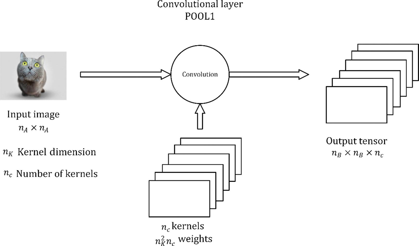
In the previous sections, I have shown you some examples of applying convolutions with just one kernel. How can you apply several kernels at the same time? Well, the answer is very simple. The final tensor (I now use the word tensor, because it will not be a simple matrix anymore) B will now have not 2 dimensions but 3. Let’s indicate the number of kernels you want to apply with nc (the c is used, because people sometimes refer to these as channels). You simply apply each filter to the input independently and stack the results. So, instead of a single matrix B with dimensions nB × nB, you get a final tensor of dimensions nB × nB × nc. That means that
will be the output of convolution of the input image with the first kernel,
will be the output of convolution with the second kernel, and so on. The convolution layer is nothing other than something that transforms the input into an output tensor. But what are the weights in this layer? The weights, or the parameter, that the network learns during the training phase, are the elements of the kernel themselves. We have discussed that we have nc kernels, each of dimensions nK × nK. That means that we have the parameter in a convolutional layer.
Note
The number of parameters that you have in a convolutional layer, , is independent of the input image size. This fact helps in reducing overfitting, especially when dealing with big size input images.
Sometimes, this layer is indicated with the word POOL and a number. In our case, we could indicate this layer with POOL1. In Figure 8-12, you can see a representation of a convolutional layer. The input image gets transformed by applying convolution with nc kernels in a tensor of dimensions nA × nA × nc.
A convolutional layer does not necessarily have to be placed immediately after the inputs. A convolutional layer may get as input the output of any other layer, of course. Keep in mind that usually your input image will have dimensions nA × nA × 3, because an image in color has three channels: RGB. A complete analysis of the tensors involved in a CNN when considering color images is beyond the scope of this book. Very often in diagrams, the layer is simply indicated as a cube or square.
.
Pooling Layers
A pooling layer is usually indicated by POOL and a number: for example, POOL1. It takes as input a tensor and gives as output another tensor, after applying pooling to the input.
Note
A pooling layer has no parameter to learn, but it introduces additional hyperparameters: nK and stride s. Typically, in pooling layers, you don’t use any padding, because one of the reasons to use pooling is often to reduce the dimensionality of the tensors.
Stacking Layers Together
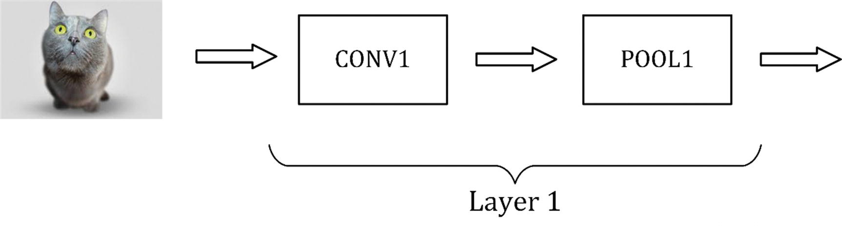
In CNNs, you usually stack convolutional and pooling layers together, one after the other. In Figure 8-13, you can see a convolutional and a pooling layer stack. A convolutional layer is always followed by a pooling layer. Sometimes, the two together are called a layer. The reason is that a pooling layer has no learnable weights, and, therefore, it is seen as a simple operation that is associated with the convolutional layer. So, be aware when you read papers or blogs, and verify what they intend.
Figure 8-13
Representation of how to stack convolutional and pooling layers
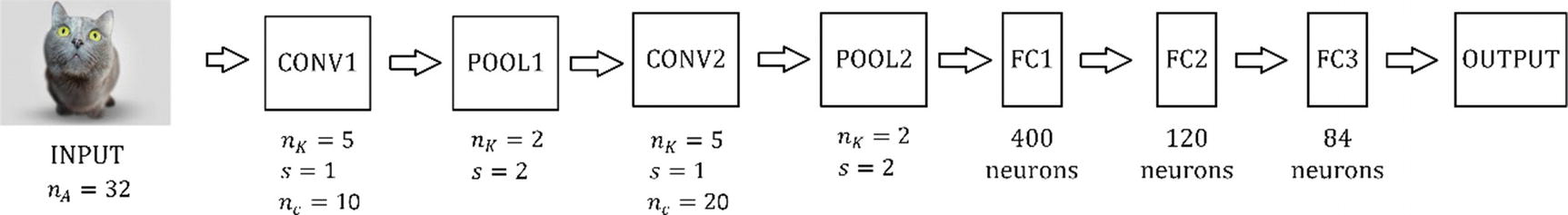
To conclude this discussion of CNNs, in Figure 8-14, you can see an example of a CNN. It is similar to the very famous LeNet-5 network, on which you can read more here: https://goo.gl/hM1kAL. You have the inputs, then two convolution-pooling layers twice, three fully connected layers, and an output layer, in which you may have your softmax function, in case, for example, you perform multiclass classification. I put some arbitrary numbers in the figure, to give you an idea of the size of the different layers.
Figure 8-14
Representation of a CNN similar to the famous LeNet-5 network
Example of a CNN
Let’s try to build one such network, to give you a feel for how the process would work and what the code looks like. We will not do any hyperparameter tuning or optimization, to keep the section understandable. We will build the following architecture with the following layers, in this order:
Convolution layer 1, with six filters 5 × 5, stride s = 1
Max pooling layer 1, with a window 2 × 2, stride s = 2
We then apply ReLU to the output of the previous layer.
Convolution layer 2, with 16 filters 5 × 5, stride s = 1
Max pooling layer 2, with a window 2 × 2, stride s = 2
We then apply ReLU to the output of the previous layer.
Fully connected layer, with 128 neurons and activation function ReLU
Fully connected layer, with 10 neurons for classification of the Zalando dataset
Softmax output neuron
We will import the Zalando dataset, as we did in Chapter 3, as follows:
Note that in this case, unlike in Chapter 3, we will use the transpose of all tensors, meaning that in each row, we will have an observation. In Chapter 3, each observation was in a column. If you check the dimensions with the code
print(labels_.shape)
print(labels_dev_.shape)
you will get the following results:
(60000, 10)
(10000, 10)
In Chapter 3, the dimensions were exchanged. The reason is that to develop the convolutional and pooling layers, we will use functions that are provided by TensorFlow, because developing them from scratch would require too much time. In addition, for some TensorFlow functions, it is easier if the tensors have different observations along the rows. As in Chapter 3, we must normalize the data.
train = np.array(train / 255.0)
dev = np.array(dev / 255.0)
labels_ = np.array(labels_)
labels_test_ = np.array(labels_test_)
We can now start to build our network.
x = tf.placeholder(tf.float32, shape=[None, 28*28])
The one line that requires an explanation is the second: x_image = tf.reshape(x, [-1, 28, 28, 1]). Remember that the convolutional layer will require the two-dimensional image and not a flattened list of gray values of the pixel, as was the case in Chapter 3, where our input was a vector with 784 (28 × 28) elements.
Note
One of the biggest advantages of CNNs is that they use the two-dimensional information contained in the input image. This is why the input of convolutional layers are two-dimensional images and not a flattened vector.
When building CNNs, it is typical to define functions to build the different layers. In this way, hyperparameter tuning later will be easier, as we have seen previously. Another reason is that when we put all the pieces together with the functions, the code will be much more readable. The function names should be self-explanatory. Let’s start with a function to build the convolutional layer. Note that TensorFlow documentation uses the term filter, so this is what we will use in the code.
At this point, we will initialize the weights from a truncated normal distribution, the biases as a constant, and then we will use stride s = 1. The stride is a list, because it gives the stride in different dimensions. In our examples, we have gray images, but we could also have RGB, for example, thereby having more dimensions: the three color channels.
The pooling layer is easier, since it has no weights.
The new TensorFlow functions that we have used are tf.nn.conv2d, which builds a convolutional layer, and tf.nn.max_pool, which builds a pooling layer with max pooling, as you can imagine from the name. We don’t have the space here to go into detail in what each function does, but you can find a lot of information in the official documentation. Now let’s put everything together and actually build the network described at the beginning.
Now let’s evaluate the predictions, to be able to evaluate the accuracy later.
y_pred = tf.nn.softmax(layer_fc2)
y_pred_scalar = tf.argmax(y_pred, axis=1)
The array y_pred_scalar will contain the class number as a scalar. Now we need to define the cost function, and, again, we will use an existing TensorFlow function to make our life easier, and to keep the length of this chapter reasonable.
It is time to train our network. We will use mini-batch gradient descent with a batch size of 100 and train our network for just ten epochs. We can define the variables as follows:
If you run this code (it took roughly ten minutes on my laptop), it will start, after just one epoch, with a training accuracy of 63.7%, and after ten epochs, it will reach a training accuracy of 86% (also on the dev set). Remember that with the first dumb network we developed in Chapter 3 with five neurons in one layer, we reached 66% with mini-batch gradient descent. We have trained our network here only for ten epochs. You can get much higher accuracy if you train longer. Additionally, note that we have not done any hyperparameter tuning, so this would get you much better results, if you spent time tuning the parameters.
As you may have noticed, every time you introduce a convolutional layer, you will introduce new hyperparameters for each layer.
Kernel size
Stride
Padding
These will have to be tuned, to get optimal results. Typically, researchers tend to use existing architectures for specific tasks that already have been optimized by other practitioners and are well documented in papers.
Introduction to RNNs
RNNs are very different from CNNs and, typically, are used when dealing with sequential information, in other words, for data for which the order matters. The typical example given is a series of words in a sentence. You can easily understand how the order of words in a sentence can make a big difference. For example, saying “the man ate the rabbit” has a different meaning than “the rabbit ate the man,” the only difference being the order of the words, and who gets eaten by whom. You can use RNNs to predict, for example, the subsequent word in a sentence. Take, for example, the phrase “Paris is the capital of.” It is easy to complete the sentence with “France,” which means that there is information about the final word of the sentence encoded in the previous words, and that information is what RNNs exploit to predict the subsequent terms in a sequence. The name recurrent comes from how these networks work: they apply the same operation on each element of the sequence, accumulating information about the previous terms. To summarize
RNNs make use of sequential data and use the information encoded in the order of the terms in the sequence.
RNNs apply the same kind of operation to all terms in the sequence and build a memory of the previous terms in the sequence, to predict the next term.
Before trying to understand a bit better how RNNs work, let’s consider a few important use cases in which they can be applied, to give you an idea of the potential range of applications.
Generating text: Predicting probability of words, given a previous set of words. For example, you can easily generate text that looks like Shakespeare with RNNs, as A. Karpathy has done on his blog, available at https://goo.gl/FodLp5.
Translation: Given a set of words in a language, you can get words in a different language.
Speech recognition: Given a series of audio signals (words), we can predict the sequence of letters forming the words as spoken.
Generating image labels: With CNNs, RNNs can be used to generate labels for images. Refer to A. Karpathy’s paper on the subject: “Deep Visual-Semantic Alignments for Generating Image Descriptions,” available at https://goo.gl/8Ja3n2. Be aware that this is a rather advanced paper that requires an extensive mathematical background.
Chatbots: With a sequence of words given as input, RNNs try to generate answers to the input.
As you can imagine, to implement the preceding, you would require sophisticated architectures that are not easy to describe in a few sentences and call for a deeper (pun intended) understanding of how RNNs work, which is beyond the scope of this chapter and book.
Notation
Let’s consider the sequence “Paris is the capital of France.” This sentence will be fed to a RNN one word at a time: first “Paris,” then “is”, then “the,” and so on. In our example,
“Paris” will be the first word of the sequence: w1 = 'Paris'
“is” will be the second word of the sequence: w2 = 'is'
“the” will be the third word of the sequence: w3 = 'the'
“capital” will be the fourth word of the sequence: w4 = 'capital'
“of” will be the fifth word of the sequence: w5 = 'of'
“France” will be the sixth word of the sequence: w6 = 'France'
The words will be fed into the RNN in the following order: w1, w2, w3, w4, w5, and w6. The different words will be processed by the network one after the other, or, as some like to say, at different time points. Usually, it is said that if word w1 is processed at time t, then w2 is processed at time t + 1, w3 at time t + 2, and so on. The time t is not related to a real time but is meant to suggest the fact that each element in the sequence is processed sequentially and not in parallel. The time t is also not related to computing time or anything related to it. And the increment of 1 in t + 1 does not have any meaning. It simply means that we are talking about the next element in our sequence. You may find the following notations when reading papers, blogs, or books:
xt: the input at time t. For example, w1 could be the input at time 1 x1, w2 at time 2 x2, and so on.
st: This the notation with which the internal memory, that we have not defined yet, at time t is indicated. This quantity st contains the accumulated information on the previous terms in the sequence discussed previously. An intuitive understanding of it will have to suffice, because a more mathematical definition would require too detailed an explanation.
ot is the output of the network at time t or, in other words, after all the elements of the sequence until t, including the element xt, have been fed to the network.
Basic Idea of RNNs
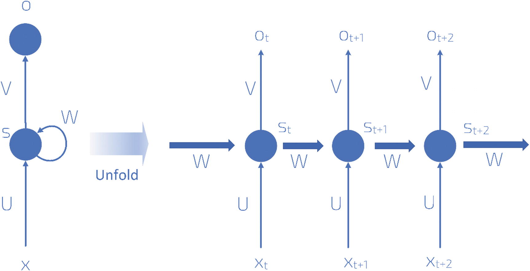
Typically, an RNN is indicated in the literature as the leftmost part of what is illustrated in Figure 8-15. The notation used is indicative—it simply indicates the different elements of the network: x refers to the inputs, s to the internal memory, W to one set of weights, and U to another set of weights. In reality, this schematic representation is simply a way of depicting the real structure of the network, which you can see at the right of Figure 8-15. Sometimes, this is called the unfolded version of the network.
Figure 8-15
Schematic representation of an RNN
The right part of Figure 8-15 should be read left to right. The first neuron in the figure does its evaluation at an indicated time t, produces an output ot, and creates an internal memory statest. The second neuron, which evaluates at a time t + 1, after the first neuron, gets as input both the next element in the sequence, xt + 1, and the previous memory state, st. The second neuron then generates an output, ot + 1, and a new internal memory state, st + 1. The third neuron (the one at the extreme right of Figure 8-15) then gets as input the new element of the sequence xt + 2 and the previous internal memory state st + 1, and the process proceeds in this way for a finite number of neurons. You can see in Figure 8-15 that there are two sets of weights: W and U. One set (indicated by W) is used for the internal memory states, and one, U, for the sequence element. Typically, each neuron will generate the new internal memory state with a formula that will looks like this:
where we have indicated with f() one of the activation functions, we have already seen as ReLU or tanh. Additionally, the previous formula will, of course, be multidimensional. st can be understood as the memory of the network at time t. The number of neurons (or time steps) that can be used is a new hyperparameter that must be tuned, depending on the problem. Research has shown that when this number is too big, the network has big problems during training.
Something very important to note is that at each time step, the weights do not change. The same operation is being performed at each step, simply changing the inputs every time an evaluation is performed. Additionally, in Figure 8-15, I have an output in the diagram (ot, ot + 1 and ot + 2) for every step, but, typically, this is not necessary. In our example, in which we want to predict the final word in a sentence, we may only require the final output.
Why the Name Recurrent?
I would like to discuss very briefly why the networks are called recurrent. I have said that the internal memory state at a time t is given by
The internal memory state at time t is evaluated using the same memory state at time t − 1, the one at time t − 1 with the value at time t − 2, and so on. This is at the origin of the name recurrent.
Learning to Count
To give you an idea of their power, I would like to give you a very basic example of something RNNs are very good at and standard fully connected networks, such as the one you saw in the previous chapters, are really bad at. Let’s try to teach a network to count. The problem we want to solve is the following: given a certain vector, which we will assume as being made of 15 elements and containing just 0 and 1, we want to build a neural network that is able to count the amount of 1s we have in the vector. This is a difficult problem for a standard network, but why? To understand intuitively why, let’s consider the problem we have analyzed of distinguishing the one and two digits in the MNIST dataset.
If you remember that discussion of metric analysis, you will recall that the learning happens because the ones and the twos have black pixels in fundamentally different positions. A digit one will always differ (at least in the MNIST dataset) in the same way as the digit two, so the network identifies these differences, and as soon as they are detected, a clear identification can be made. In our case, this is no longer possible. Consider, for example, the simpler case of a vector with just five elements.
In this case, a one appears exactly one time. We have five possible cases: [1,0,0,0,0], [0,1,0,0,0], [0,0,1,0,0], [0,0,0,1,0], and [0,0,0,0,1]. There is no discernible pattern to be detected here. There is no easy weight configuration that could cover these cases at the same time. In the case of an image, this problem is similar to the problem of detecting the position of a black square in a white image. We can build a network in TensorFlow and check how good such networks are. Owing to the introductory nature of this chapter, however, I will not spend time on a discussion of hyperparameters, metric analysis, and so on. I will simply give you a basic network that can count.
Let’s start by creating our vectors. We will create 105 vectors, which we will split into training and dev sets.
import numpy as np
import tensorflow as tf
from random import shuffle
Now let’s create our list of vectors. The code is slightly more complicated, and we will look at it in a bit more detail.
nn = 15
ll = 2**15
train_input = ['{0:015b}'.format(i) for i in range(ll)]
shuffle(train_input)
train_input = [map(int,i) for i in train_input]
temp = []
for i in train_input:
temp_list = []
for j in i:
temp_list.append([j])
temp.append(np.array(temp_list))
train_input = temp
We want to have all possible combinations of 1 and 0 in vectors of 15 elements. So, an easy way to do this is to take all numbers up to 215 in a binary format. To understand why, let’s suppose we want to do this with only four elements: we want all possible combinations of four 0 and 1. Consider all numbers up to 24 in binary that you can get with this code:
['{0:04b}'.format(i) for i in range(2**4)]
The code simply formats all the numbers that you get with the range(2**4) function, from 0 to 2**4, in binary format, with {0:04b}, limiting the number of digits to 4. The result is the following:
['0000',
'0001',
'0010',
'0011',
'0100',
'0101',
'0110',
'0111',
'1000',
'1001',
'1010',
'1011',
'1100',
'1101',
'1110',
'1111']
As you can easily verify, all possible combinations are listed. You have all possible combinations of the one appearing one time ([0001], [0010], [0100], and [1000]), of the ones appearing two times, and so on. For our example, we will simply do this with 15 digits, which means that we will do it with numbers up to 215. The rest of the preceding code is there to simply transform a string such as '0100' in a list [0,1,0,0] and then concatenate all the lists with all the possible combinations. If you check the dimension of the output array, you will notice that you get (32768, 15, 1). Each observation is an array of dimensions (15, 1). Then we prepare the target variable, a one-hot encoded version of the counts. This means that if we have an input with four ones in the vector, our target vector will look like [0,0,0,0,1,0,0,0,0,0,0,0,0,0,0,0]. As expected, the train_output array will have the dimensions (32768, 16). Now let’s build our target variables.
train_output = []
for i in train_input:
count = 0
for j in i:
if j[0] == 1:
count+=1
temp_list = ([0]*(nn+1))
temp_list[count]=1
train_output.append(temp_list)
Now let’s split our set into a train and a dev set, as we have done now several times. We will do it here in a “dumb” way.
train_obs = ll-2000
dev_input = train_input[train_obs:]
dev_output = train_output[train_obs:]
train_input = train_input[:train_obs]
train_output = train_output[:train_obs]
Remember that this will work, because we have shuffled the vectors at the beginning, so we should have a random distribution of cases. We will use 2000 cases for the dev set and the rest (roughly 30,000) for the training. The train_input will have dimensions (30768, 15, 1), and the dev_input will have dimensions (2000, 15,1).
Now you can build a network with this code, and you should be able to understand almost all of it.
val, state = tf.nn.dynamic_rnn(RNN_cell, data, dtype=tf.float32)
val = tf.transpose(val, [1, 0, 2])
last = tf.gather(val, int(val.get_shape()[0]) - 1)
For performance reasons, and to let you realize how efficient RNNs are, I am using here a long short-term memory (LSTM) kind of neuron. This has a special way of calculating the internal state. A discussion of LSTMs is well beyond the scope of this book. For the moment, you should focus on the results and not on the code. If you let the code run, you will get the following result:
Epoch 0 error 80.1%
Epoch 10 error 27.5%
Epoch 20 error 8.2%
Epoch 30 error 3.8%
Epoch 40 error 3.1%
Epoch 50 error 2.0%
After just 50 epochs, the network is right in 98% of the cases. Just let it run for more epochs, and you can reach incredible precision. After 100 epochs, you can achieve an error of 0.5%. An instructive exercise is to attempt to train a fully connected network (as the ones we have discussed so far) to count. You will see how this is not possible.
You should now have a basic understanding of how CNNs and RNNs work, and on what principles they operate. The research on those networks is immense, since they are really flexible, but the discussion in the previous sections should have given you enough information to understand how these architectures work.


 , for example, you can see in Figure 8-2 which element of A gets multiplied by which element in
  and the result for the element B1, that is nothing else as the sum of all the multiplications

 can be seen intuitively in Figure 8-4. If s > 1, what can happen, depending on the dimensions of A, is that at a certain point, you cannot shift your window on matrix A (the black square in Figure 8-3, for example) anymore, and you cannot cover all of matrix A completely. In Figure 8-4, you can see how you would need an additional column on the right of matrix A (marked by many Xs), to be able to perform the convolution operation. In Figure 8-4, s = 3, and since we have nA = 5 and nK = 3, B will a scalar as a result.


 will detect the horizontal edges. This can be applied with the code
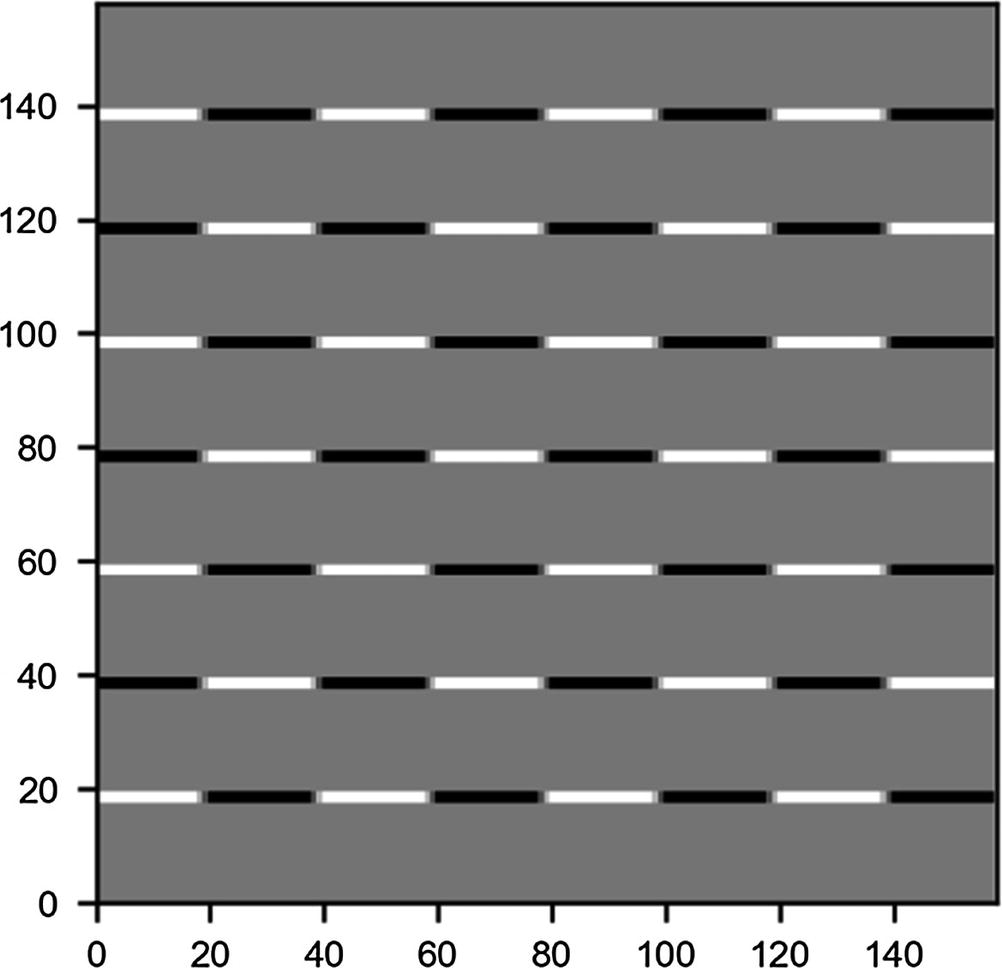
 and the chessboard image
![$$ {n}_B=left[frac{n_A-{n}_K}{s}+1
ight]=left[frac{160-3}{1}+1
ight]=left[frac{157}{1}+1
ight]=left[158
ight]=158 $$](http://images-20200215.ebookreading.net/10/2/2/9781484237908/9781484237908__applied-deep-learning__9781484237908__images__463356_1_En_8_Chapter__463356_1_En_8_Chapter_TeX_Equag.png)
 with the code
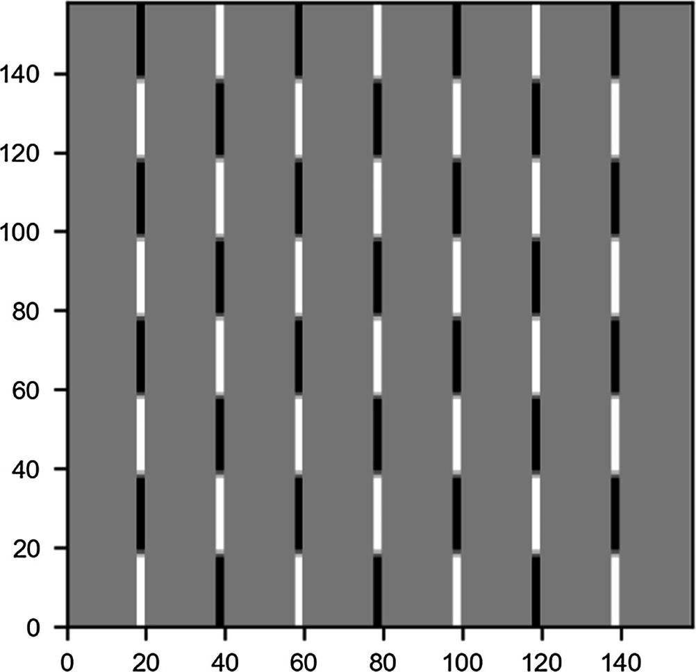
 and the chessboard image
 and the chessboard image
 .
.
 . On the left is the blurred image, and on the right, the original one.
 . We can perform the convolution with the code
 has clearly detected the sharp transition in the original matrix, marking with a vertical black line where the transition from black to white occurs. For example, consider B11 = 0.


 , as described in the text


 of dimensions nB × nB × nc. That means that
![$$ { ilde{B}}_{i,j,1}kern1em forall i,jin left[1,{n}_B
ight] $$](http://images-20200215.ebookreading.net/10/2/2/9781484237908/9781484237908__applied-deep-learning__9781484237908__images__463356_1_En_8_Chapter__463356_1_En_8_Chapter_TeX_Equbb.png)
![$$ { ilde{B}}_{i,j,2}kern1em forall i,jin left[1,{n}_B
ight] $$](http://images-20200215.ebookreading.net/10/2/2/9781484237908/9781484237908__applied-deep-learning__9781484237908__images__463356_1_En_8_Chapter__463356_1_En_8_Chapter_TeX_Equbc.png)
 parameter in a convolutional layer.
 , is independent of the input image size. This fact helps in reducing overfitting, especially when dealing with big size input images.