In this chapter, you will look at the problem of finding the best hyperparameters to get the best results from your models. First, I will describe what a black-box optimization problem is, and how that class of problems relate to hyperparameter tuning. You will see the three best-known methods to tackle these kind of problems: grid search, random search, and Bayesian optimization. I will show you, with examples, which one works under which conditions, and I will give you a few tricks that are very helpful for improving optimization and sampling on a logarithmic scale. At the end of the chapter, I will show you how you can use those techniques to tune a deep model, using the Zalando dataset.
Black-Box Optimization

Finding the hyperparameter for a given machine-learning model that maximizes the chosen optimizing metric
Finding the maximum or minimum of a function that can only be evaluated numerically or with code that we cannot look at. In some industry contexts, there can be legacy code that is very complicated, and there are some functions that must be maximized, based on its outcome.
Finding the best place to drill for oil. In this case, your function would be how much oil you can find and x your location.
Finding the best combination of parameters for situations that are too complex to model, for example, when launching a rocket in space, how to optimize the amount of fuel, diameter of each stage of the rocket, precise trajectory, etc.
This is a very fascinating class of problems, which has produced smart solutions. You will see three of them: grid search, random search, and Bayesian optimization. If you are curious about the subject, you can check out the black-box optimization competition at https://goo.gl/LY7huY . The rules of the competition mirror real-life problems. A problem is set up for which you must optimize a function (find the maximum or minimum) through a black-box interface . You can get the value of the function for all values of x, but you cannot get any other information, as its gradients, for example.
Why does finding the best hyperparameters for neural networks constitute a black-box problem? Because we cannot calculate information, such as the gradients of our network output, with respect to the hyperparameters, especially when using complex optimizers or custom functions, we require other approaches, to be able to find the best hyperparameters that maximize the chosen optimizing metric. Note that if we could have the gradients, we could use an algorithm as the gradient descent to find the maximum or minimum.
Note
Our black-box function f will be our neural network model (including things such as the optimizer, cost function form, etc.) that gives as output our optimizing metric, given the hyperparameters as input, and x will be the array containing the hyperparameters.
Learning rate: Suppose we want to try the values n · 10−4 for n = 1, …, 102. (100 values)
Regularization parameter: 0, 0.1, 0.2, 0.3, 0.4, and 0.5 (6 values)
Choice of optimizer: GD, RMSProp, or Adam (3 values)
Number of hidden layers: 1, 2, 3, 5, and 10 (5 values)
Number of neurons in the hidden layers: 100, 200, and 300 (3 values)

times, if you want to test all possible combinations. If your training takes 5 minutes, you will require 13.4 weeks of computing time. If the training takes hours or days, you will not have any chance. If the training takes one day, for example, you will require 73.9 years to try all possibilities. Most of the hyperparameter choices will come from experience. For example, you can always use Adam safely, because it is the better optimizer available (in almost all cases). But you will not be able to avoid trying to tune other parameters, such as the number of hidden layers or learning rate. You can reduce the number of combinations you need with experience (as with the optimizer), or with some smart algorithm, as you will see later in this chapter.
Notes on Black-Box Functions
Cheap functions: Functions that can be evaluated thousands of times
Costly functions: Functions that can only be evaluated a few times, usually less than 100 times
If the black-box function is cheap, the choice of the optimization method is not critical. For example, we can evaluate the gradient with respect to the x numerically, or simply search the maximum evaluating the functions on a high number of points. If the function is costly, we need much smarter approaches. One of these is Bayesian optimization, which I will discuss later in this chapter, to give you an idea of how these methods work and how complex they are.
Note
Especially in the deep-learning world, neural networks are almost always costly functions.
For costly functions, we must find methods that solve our problem with the smallest number of evaluations possible.
The Problem of Hyperparameter Tuning
Number of epochs : Sometimes, simply training your network longer will give you better results.
Choice of optimizer : You can try choosing a different optimizer. If you are using plain gradient descent, you may try Adam and see if you get better results.
Varying the regularization method : As discussed previously, there are several ways of applying regularization. Varying the method may well be worth trying.
Choice of activation function : Although the activation function always used in the previous chapters for neurons in hidden layers was ReLU, others may work a lot better. Trying sigmoid or Swish, for example, may help you get better results.
Number of layers and number of neurons in each layer: try different configurations: Try layers with different numbers of neurons, for example.
Learning rate decay methods : Try (if you are not using optimizers that do this already) different learning rate decay methods.
Mini-batch size : Vary the size of mini-batches. When you have little data, you can use batch gradient descent. When you have a lot of data, mini-batches are more efficient.
Weight initialization methods
Parameters that are continuous real numbers or, in other words, that can assume any value. Example: learning rate, regularization parameter
Parameters that are discrete but can theoretically assume an infinite number of values. Example: number of hidden layers, number of neurons in each layer, or number of epochs
Parameters that are discrete and can only assume a finite number of possibilities. Example: optimizer, activation function, learning rate decay method.
For category 3, there is not much to do except try all possibilities. Typically, these parameters will completely change the model itself, and, therefore, it is impossible to model their effects, making a test the only possibility. This is also the category for which experience may help the most. It is widely known that the Adam optimizer is almost always the best choice, for example, so you may concentrate your efforts somewhere else at the beginning. For categories 1 and 2, this is a bit more difficult, and we will have to come up with some smart ideas to find the best values.
Sample Black-Box Problem

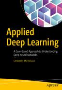
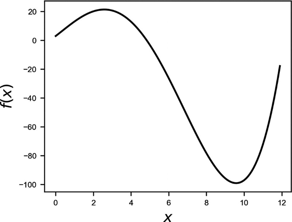
Plot of the function f(x), as described in the text
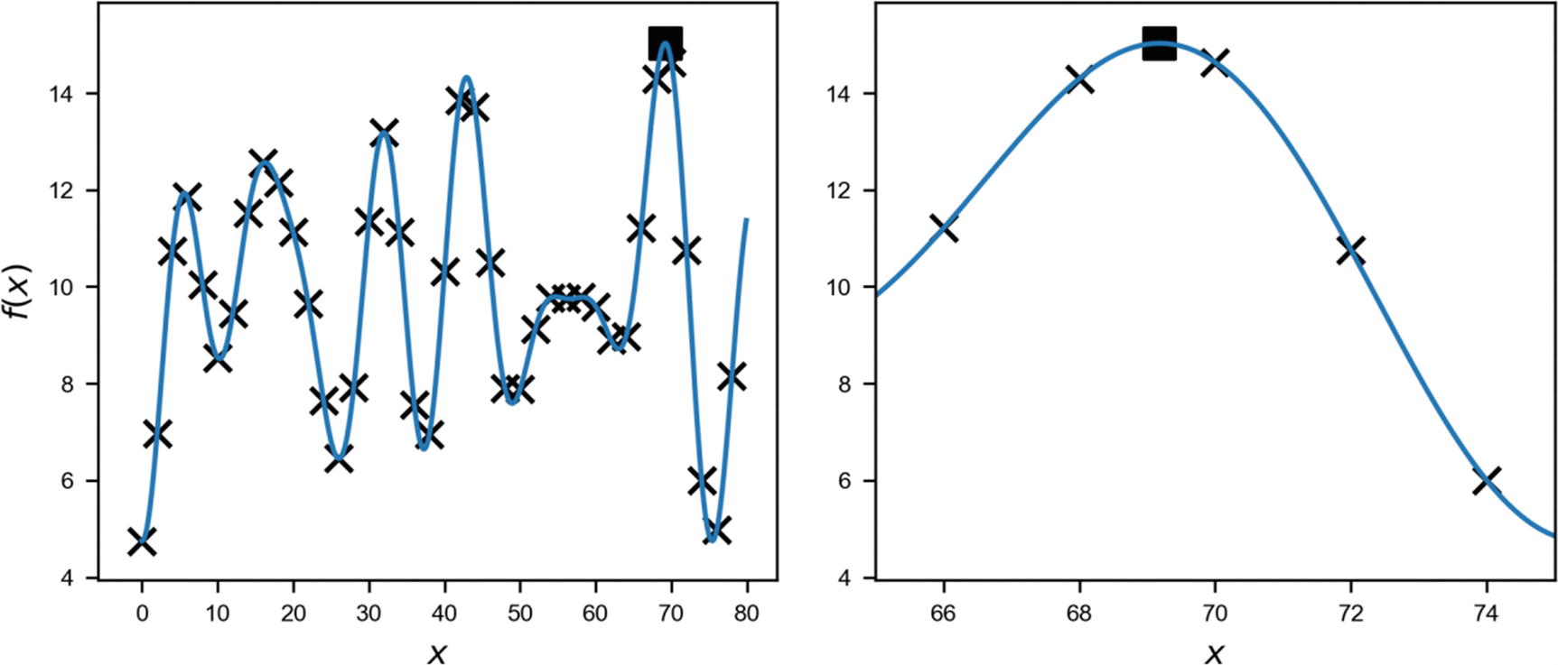
The maximum is at an approximate value x = 69.18 and has a value of 15.027. Our challenge is to find this maximum in the most efficient way possible, without knowing anything about f(x), except its value at any point we want. When we say “efficient,” we mean, of course, with the smallest number of evaluations possible.
Grid Search


 will then be
 , we will also have
 . We can create the vector x easily in Python with the following code:
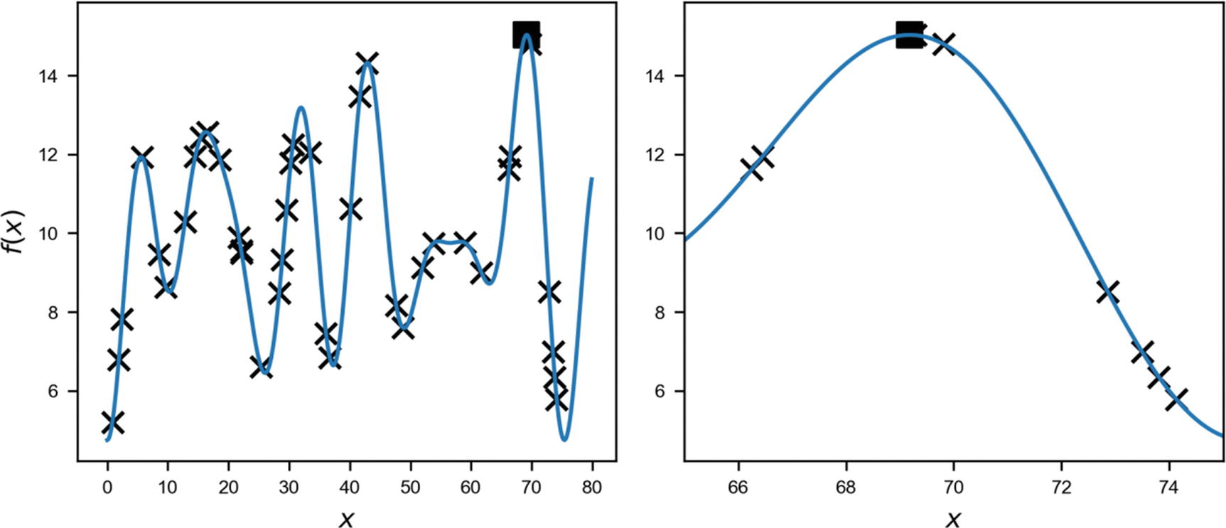
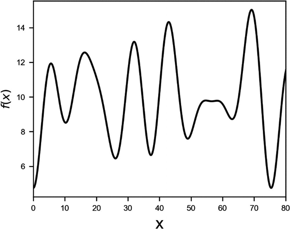
Function f(x) on the range [0, 80]. The crosses mark the point we sample in the grid search, and the black square marks the maximum.
 easily with the trivial code
In the lists xlistg and flistg, we will find the position of the maximum found and the value of the maximum for the various values of n.
Distribution of the results for  obtained by varying the number of points n sampled in the grid search. The black vertical line indicates the real maximum of f(x).
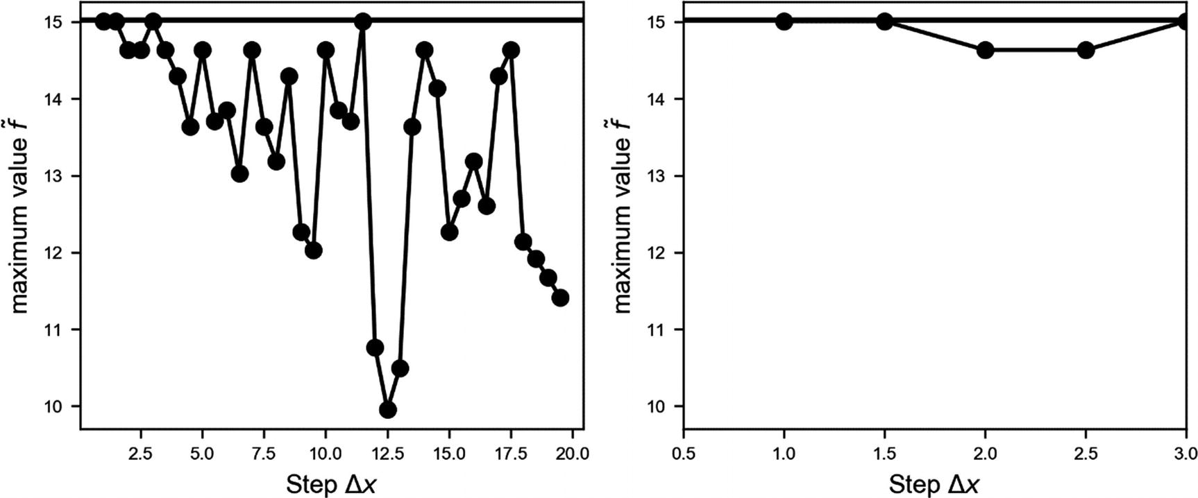
Behavior of the found value of the maximum vs. the x step Δx
In the zoom in the right plot in Figure 7-4, it is evident how smaller values of Δx get you better values of  . Note that a step of 1.0 means sampling 80 values of f(x). If, for example, the evaluation takes 1 day, you will have to wait 80 days to get all the measurements you require.
Note
Grid search is a method that is efficient only when the black-box function is cheap. To get good results, a big number of sampling points is usually needed.
To make sure you are really getting the maximum, you should decrease the step Δx, or increase the number of sampling points, until the maximum value you find does not change appreciably anymore. In the preceding example, as you see from the right plot in Figure 7-4, we are sure we are close to the maximum when our step Δx gets smaller than roughly 2.0, or, in other words, when the number of sampled points is greater or roughly equal to 40. Remember: 40 may seem quite a small number at first sight, but if f(x) evaluates the metric of your deep-learning model, and the training takes 2 hours, for example, you are looking at 3.3 days of computer time. Normally, in the deep-learning world, 2 hours is not much for training a model, so make a quick calculation before starting a long grid search. Additionally, keep in mind that when doing hyperparameter tuning, you are moving in a multidimensional space (you are not optimizing only one parameter, but many), so the number of evaluations needed gets big very fast.
Optimizer (RMSProp, Adam, or plain GD) (3 values)
Number of epochs (1000, 5000, or 10,000) (3 values)
you are already looking at nine evaluations. How many values of the learning rate can you then afford to try? Only five! And with five values, it is not probable to get close to the optimal value. This example has the goal of helping you to understand how grid search is viable only for cheap black-box functions. Remember that often time is not the only problem. For example, if you are using the Google cloud platform to train your network, you are paying for the hardware you use by the second. Maybe you have lots of time at your disposal, but costs may exceed your budget very quickly.
Random Search
Function f(x) on the range [0, 80]. The crosses mark the point we sampled with random search, and the black square marks the maximum.
 is plotted in Figure 7-6.
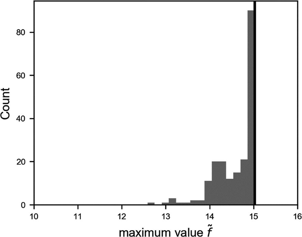
Distribution of the results for  obtained by 200 different random sets of 40 points sampled in the random search. The black vertical line indicates the real maximum of f(x).
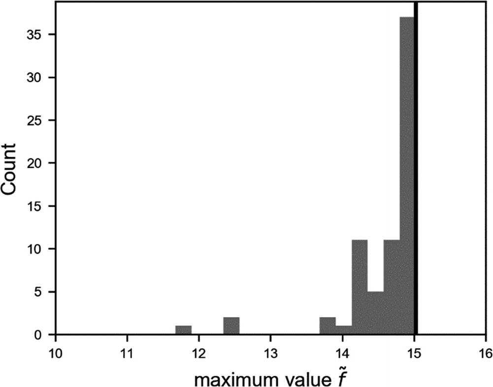
Distribution of the results for  obtained by varying the number of points n sampled in the random search, from 10 to 80. The black vertical line indicates the real maximum of f(x).
 when using a different number of sampling points n with random and grid searches. In both cases, the plots were generated with 38 different sets, so that the total count is the same.
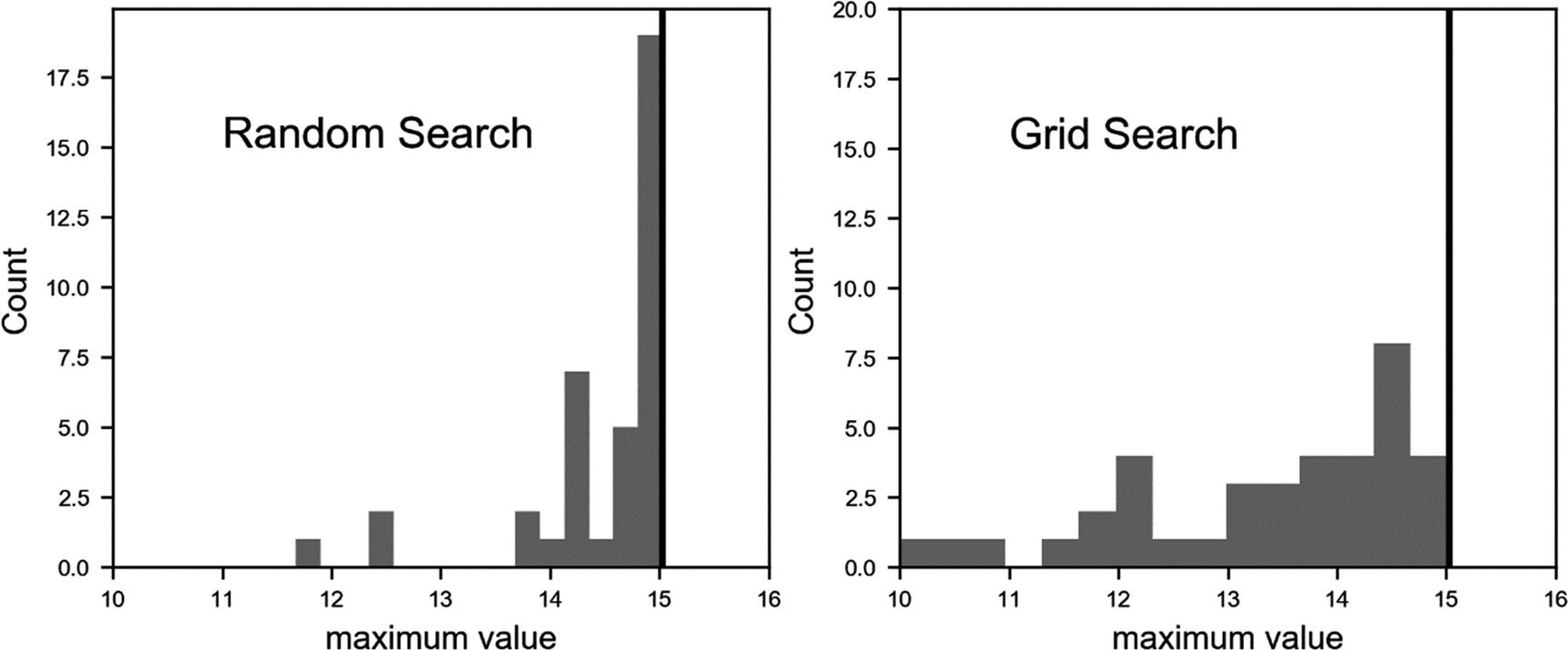
Comparison of the distribution of  between grid (right) and random (left) searches
, while varying the number of sampling points n. Both plots count sums to 38, the number of different numbers of sampling points used. The correct value of the maximum is marked by the vertical black line in both plots.
between grid (right) and random (left) searches
, while varying the number of sampling points n. Both plots count sums to 38, the number of different numbers of sampling points used. The correct value of the maximum is marked by the vertical black line in both plots.
It is easy to see how on average random search is better than grid search. The values you get are consistently closer to the right maximum.
Note
Random search is consistently better than grid search, and you should use it whenever possible. The difference between random search and grid search becomes even more marked when dealing with a multidimensional space for your variable x. Hyperparameter tuning is practically always a multidimensional optimization problem.
If you are interested in a very good paper on how random search scales for high dimensional problems, read James Bergstra and Yoshua Bengio, Random Search for Hyper-Parameter Optimization, available at https://goo.gl/efc8Qv .
Coarse-to-Fine Optimization
- 1.
Do a random search in the region R1 = (xmin, xmax). Let’s indicate the maximum found with (x1, f1).
- 2.
Consider now a smaller region around x1, R2 = (x1 − δx1, x1 + δx1), for some δx1, which I will discuss later, and again do a random search in this region. The hypothesis is, of course, that the real maximum lies in this region. We will indicate the maximum you find here with (x2, f2).
- 3.
Repeat step 2 around x2, in the region we will indicate with R3, with a δx2 smaller than δx1, and indicate the maximum you find in this step with (x3, f3).
- 4.
Now repeat step 2 around x3, in the region we will indicate with R4, with a δx3 smaller than δx2.
- 5.
Continue in the same way as often as you require, until the maximum (xi, fi) in the region Ri + 1 no longer changes.
 and take again 10 points in region R2 = (x1 − δx, x1 + δx). In the interval (x1 − δx, x1 + δx), we will have on average a distance between the points of 1% of xmax − xmin, but we just sampled our functions only 20 times, instead of 100, so by a factor 5 fewer! For example, let’s just sample the function we used previously between xmin = 0 and xmax = 80 with 10 points, with the code
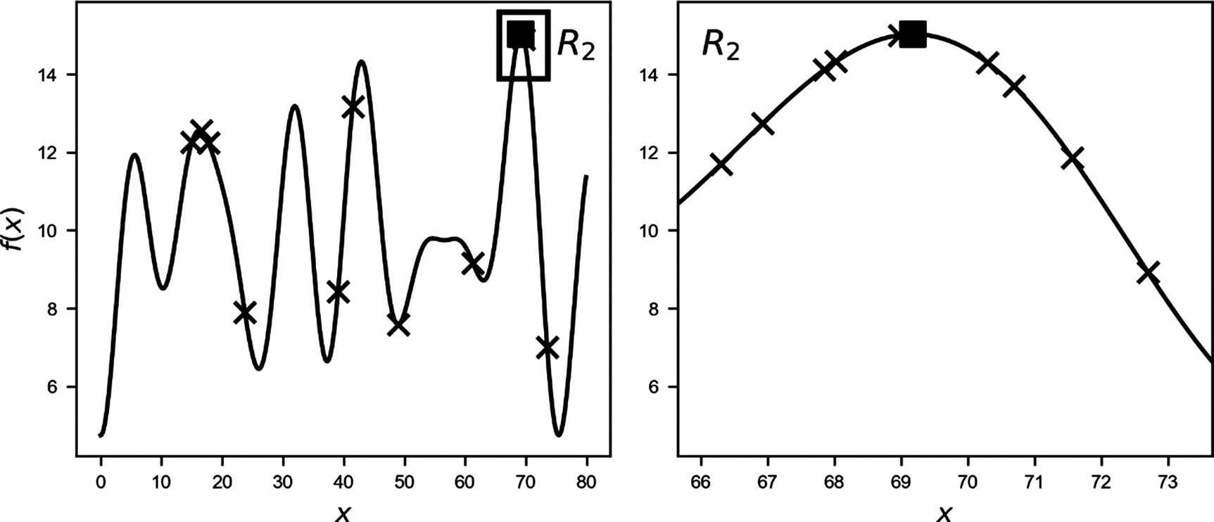
Function f(x). The crosses mark the sampled points: on the left, the 10 points sampled in the regions R1 (entire range), on the right, the 10 points sampled in R2. The black square marks the real maximum. The plot on the right is a zoom of the region R2.
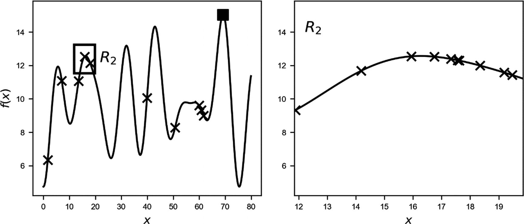
Function f(x). The crosses mark the sampled points: on the left, the 10 points sampled in the regions R1 (entire range), on the right, the 10 points sampled in R2. The black square marks the real maximum. The algorithm finds a maximum very well around 16, simply not the absolute maximum. The small rectangle on the left marks the region R2. The plot on the right is a zoom of the region R2.
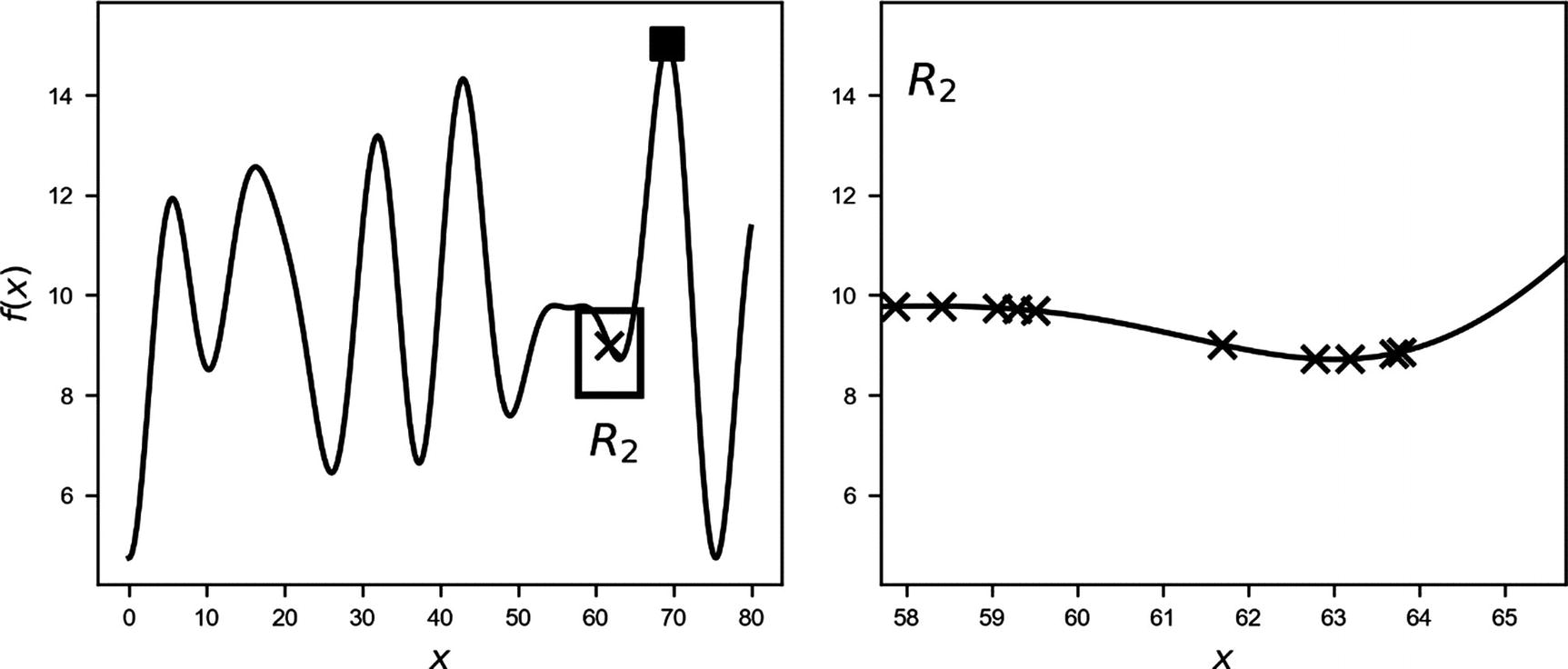
Function f(x). The crosses mark the sampled points: on the left, the 1 point is sampled in the regions R1 (entire range), on the right, the 10 points are sampled in R2. The black square marks the real maximum. The algorithm does not find any maximum, because none is present in the region R2. The plot on the right is the zoom of the region R2.
If you decide to use this method, keep in mind that you will still require a good number of points at the beginning, to get close to the maximum, before refining your search. After you are relatively sure to have points around your maximum, you can use this technique to refine your search.
Bayesian Optimization
In this section, we will look at a specific and efficient technique for finding the minimum (or maximum) of a black-box function. This is a rather clever algorithm that basically consists of choosing the sampling points from which to evaluate the function in a much more intelligent way than simply choosing them randomly or on a grid. To understand how this works, you must first look at a few new mathematical concepts, because the method is not trivial and requires some understanding of more advanced concepts. Let’s start with the Nadaraya-Watson regression.
Nadaraya-Watson Regression


The parameter l makes the Gaussian shape wider or narrower. The σ is typically the variance of your data, but, in this case, it plays no role, because the weights are normalized to one. This is at the basis of Bayesian optimization, as you will see later.
Gaussian Process

 . Remember that a random variable with a Gaussian distribution is said to be normally distributed. From this comes the name Gaussian process. The probability distribution of the normal distribution is given by the function

![$$ mathit{operatorname{cov}}left[fleft({x}_1
ight),fleft({x}_2
ight)
ight]=Kleft({x}_1,{x}_2
ight) $$](http://images-20200215.ebookreading.net/10/2/2/9781484237908/9781484237908__applied-deep-learning__9781484237908__images__463356_1_En_7_Chapter__463356_1_En_7_Chapter_TeX_Equo.png)
The choice of the letter K has a reason. We will assume in what follows that the covariance will have a Gaussian shape , and we will use for K the RBF function defined previously.
Stationary Process

Note that to apply the method we are describing, first you must convert your data to be stationary, if that is not already the case, eliminating seasonality or trends in time, for example.
Prediction with Gaussian Processes

Or, in other words, the probability of getting the value f(x), given the vector f, composed by all the points f(x1), …, f(xn).

Where, with  , we have indicated the normal distribution calculated on the points with average 0 and covariance matrix
  of dimensions n + 1 × n + 1, because we have n + 1 points in the numerator. The derivation is somewhat involved and is based on several theorems, such as Bayes’ theorem. For more information, you can refer to the (advanced) explanation by Chuong B. Do in “Gaussian Processes” (2007), available at
https://goo.gl/cEPYwX
, in which everything is explained in elaborate detail. To understand what Bayesian optimization is, we can simply use the formula without derivation. C will have dimensions n × n, because we have only n points in the denominator.
of dimensions n + 1 × n + 1, because we have n + 1 points in the numerator. The derivation is somewhat involved and is based on several theorems, such as Bayes’ theorem. For more information, you can refer to the (advanced) explanation by Chuong B. Do in “Gaussian Processes” (2007), available at
https://goo.gl/cEPYwX
, in which everything is explained in elaborate detail. To understand what Bayesian optimization is, we can simply use the formula without derivation. C will have dimensions n × n, because we have only n points in the denominator.


Plot of our unknown test function, as described in the text
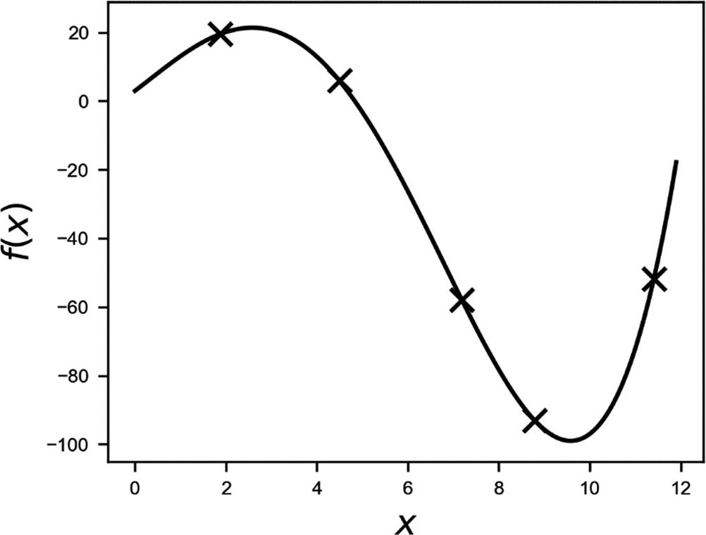
Plot of the unknown function. The crosses mark the random point chosen in the text.
We do a loop over a range of x points, where we want to evaluate our function, with the code for x in xsampling:.
We build our k and f vectors with the code for each element of the vectors: k = K(x-randompoints, 2 , sigm_) and f1 = f(randompoints). For the kernel, we have chosen a value for the parameter l, as defined in the function of 2. We have subtracted, in the vector f, the average to obtain m(x) = 0, to be able to apply the formulas as derived.
We build the matrices C and
 .
.We calculate μ with mu = np.dot(np.dot(np.transpose(k), np.linalg.inv(C)), f_) and the standard deviation.
At the end, we reapply all the transformation that we have done to make our process stationary in the opposite order, simply adding the average of f(x) again to the evaluated surrogate function ybayes = np.asarray(ybayes_)+np.average(f1).
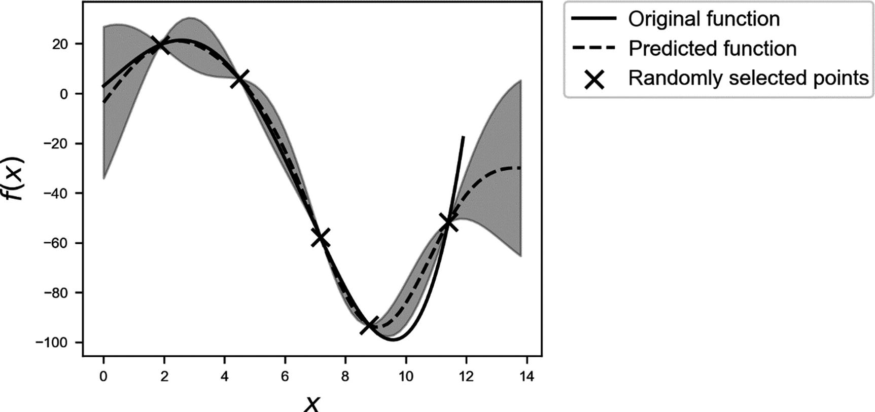
Predicted function (dashed line), calculated by evaluating μ(x). The gray area is the region between the estimated function and +/- σ.
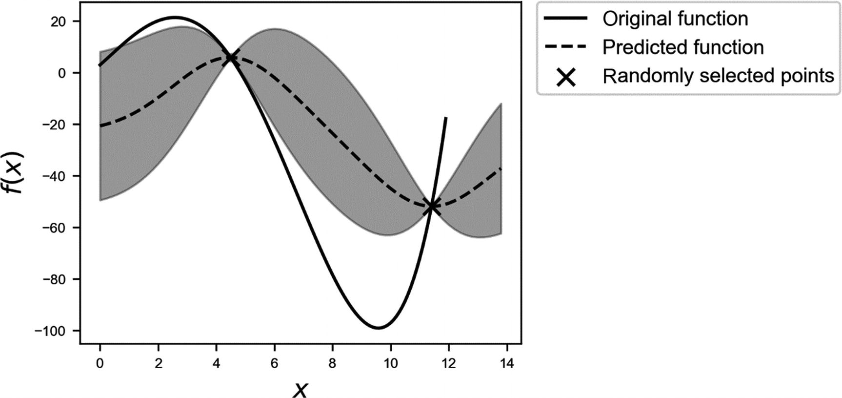
Predicted function (dashed line), when we have only two points at our disposal. The gray area is the region between the estimated function +/- σ.
 that approximates our function f and has the property
This surrogate function must have another very important property: it must be cheap to evaluate. In this way, we can find easily the maximum of  , and, using the previous property, we will have the maximum of f, which, by hypothesis, is costly.
But as you have seen, it may be very difficult to know if we have enough points to find the right value of the maximum . After all, by definition, we don’t have any idea how our black-box function looks. So, how to solve this problem?
- 1.
We start with a small number of sample points randomly chosen (how small it should be will depend on your problem).
- 2.
We use this set of points to get a surrogate function, as described.
- 3.
We add an additional point to our set, with a specific method that I will discuss later, and reevaluate the surrogate function.
- 4.
If the maximum we find with the surrogate function continues to change, we will continue adding points, as in step 3, until the maximum does not change anymore, or we run out of time or budget and cannot perform any further evaluation.
If the method I hinted at in step 3 is smart enough, we will be able to find our maximum relatively quickly and accurately.
Acquisition Function
- 1.
We choose a function (and we will see a few possibilities in a moment) called an acquisition function.
- 2.
Then we choose, as additional point x, the one at which the acquisition function has a maximum.
There are several acquisition functions we can use. I will describe here only one that we will use to see how this method works, but there are several that you may want to check out, such as entropy search, probability of improvement, expected improvement, and upper confidence bound.
Upper Confidence Bound (UCB)

where we have indicated with  the “expected” value of the surrogate function on the x-range we have in our problem. The expected value is nothing other than the average of the function over the given x range. σ(x) is the variance of the surrogate function that we calculate with our method at point x. The new point we select is the one in which aUCB(x) is maximum. η > 0 is a trade-off parameter. This acquisition function basically selects the points where the variance is biggest. Review Figure 7-15. The method selects the points at which the variance is greater, so, points as far as possible from the points we have already. In this way, the approximation tends to get better and better.

This time, the acquisition function will make a trade-off between choosing points around the surrogate function maximum and points where its variance is biggest. This second method works best to find quickly good approximation of the maximum of f, while the first tends to give good approximation of f over the entire x range. In the next section, we will see how these methods works.
Example
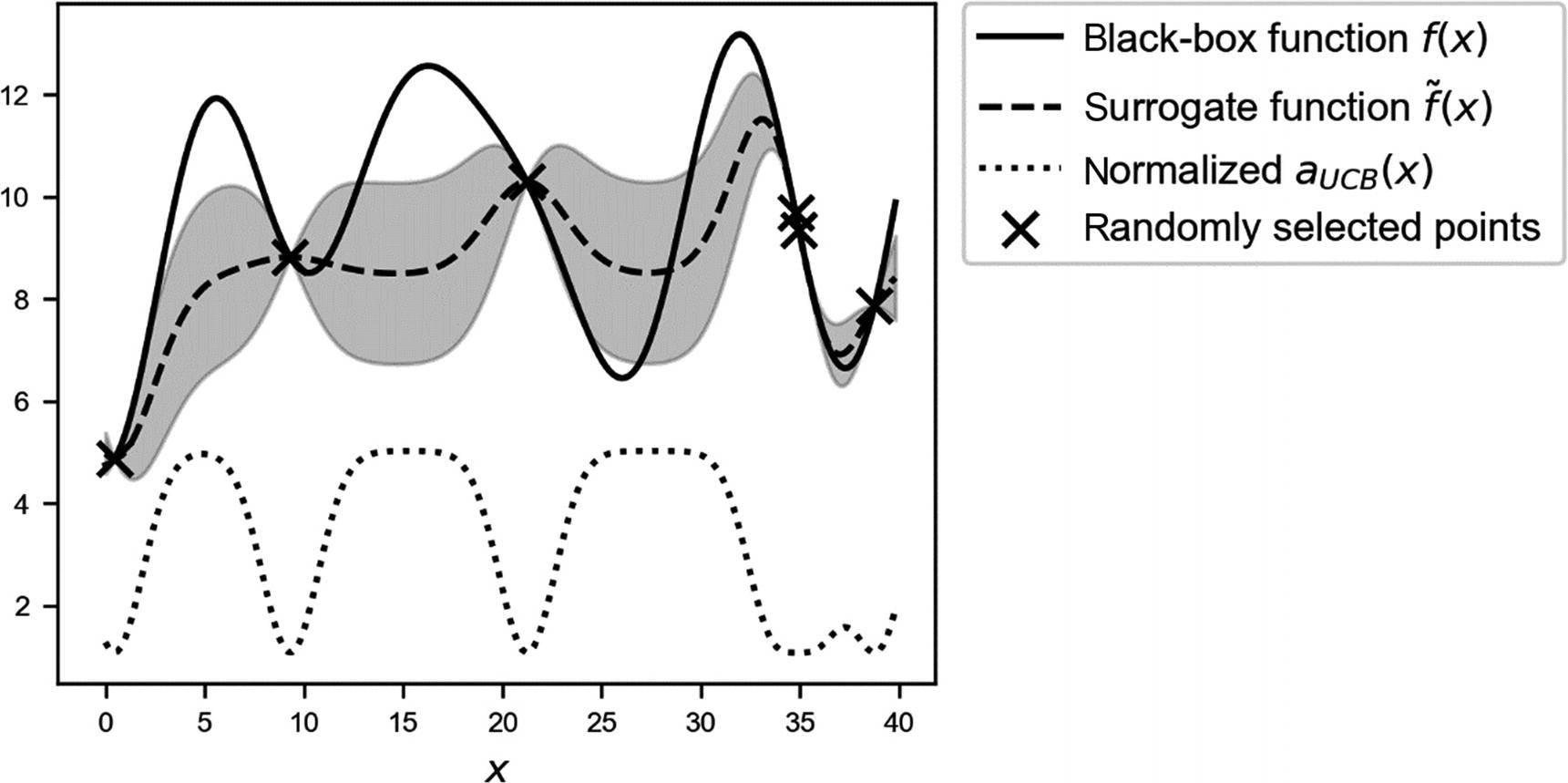
Overview of the black-box function f(x) (solid line), the randomly selected points (marked by crosses), the surrogate function (dashed line), and the acquisition function aUCB(x) (dotted line), shifted to fit in the plot. The gray area is the region contained between the lines  and
and  .
.
 and with η = 3.0.
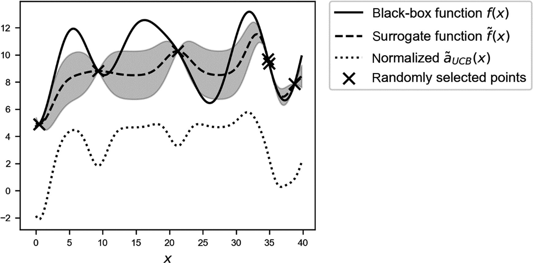
Overview of the black-box function
f(x) (solid line), the randomly selected points (marked by crosses), the surrogate function (dashed line), and the acquisition function  (dotted line), shifted to fit in the plot. The gray area is the region contained between the lines
  and
and  .
.
As you can see,  tends to have a maximum around the maximum of the surrogate function. Keep in mind that if η is big, the maximum of the acquisition function will shift toward regions with high variance. But this acquisition function tends to find “a” maximum slightly faster. I said “a,” because it depends on where the maximum of the surrogate function is, and not where the maximum of the black-box function is.
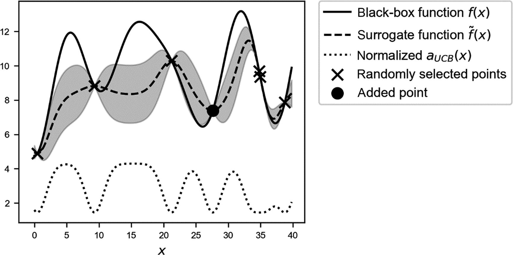
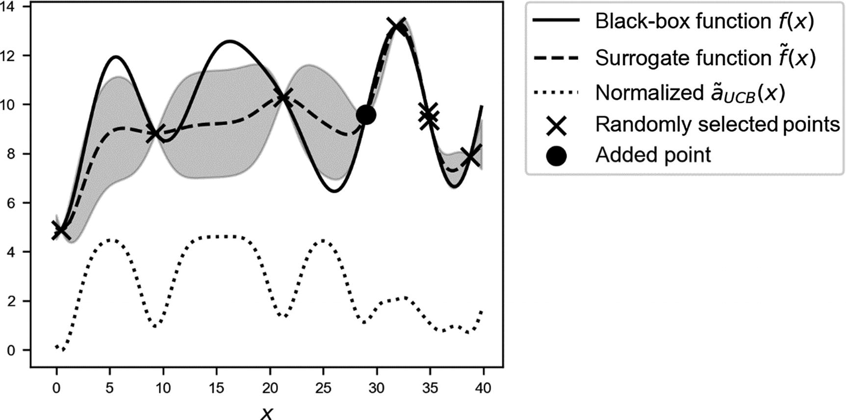
Overview of the black-box function
f(x) (solid line), the randomly selected points (marked with crosses), and with the new selected point around x ≈ 27 (marked by a circle), the surrogate function (dashed line), and the acquisition function aUCB(x) (dotted line), shifted to fit in the plot. The gray area is the region contained between the lines  and
and  .
.
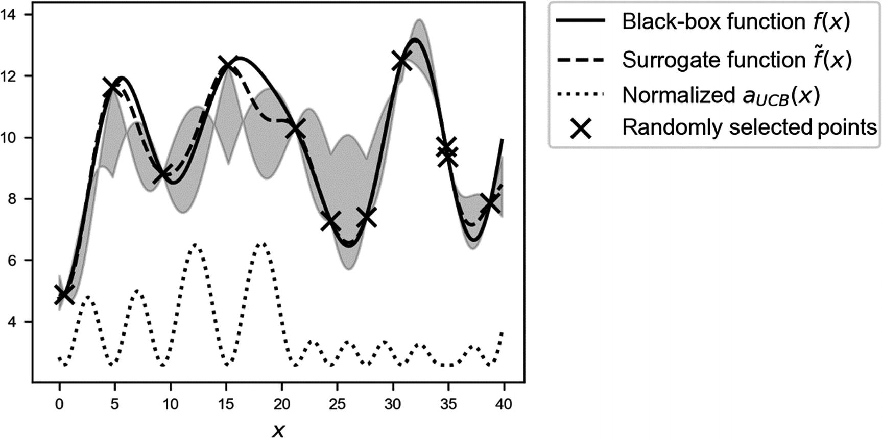
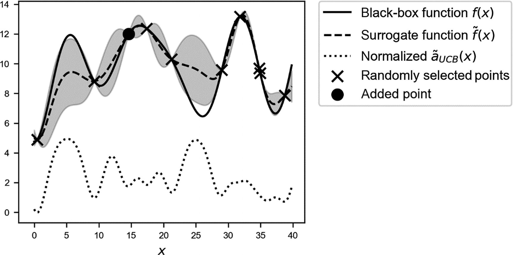
Overview of the black-box function
f(x) (solid line), the randomly selected points with the six selected new points (marked by crosses), the surrogate function (dashed line), and the acquisition function  (dotted line), shifted to fit in the plot. The gray area is the region contained between the lines
  and
and  .
.
Note the dashed line. Now our surrogate function approximates the black-box function quite well, especially around the real maximum. Using this surrogate function, we can find a very good approximation of our original function with just 11 evaluations in total! Keep in mind that we don’t have any additional information about f, except the 11 evaluations.
 , and let’s check how fast we can find the maximum. In this case, we’ll use η = 3.0, to get a better balance between the maximum of the surrogate function and its variance. In Figure 7-20, you can see the result after just adding one single additional point, marked by a black circle. We have already a quite good approximation of the real maximum!
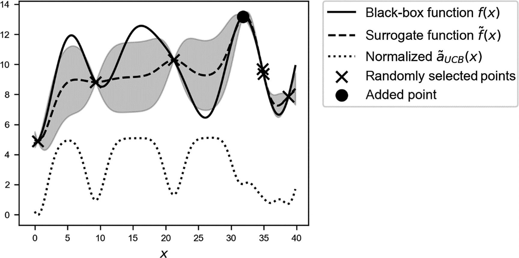
Overview of the black-box function
f(x) (solid line), the randomly selected points with the additional selected points (marked by crosses), the surrogate function (dashed line), and the acquisition function  (dotted line), shifted to fit in the plot. The gray area is the region contained between the lines
  and
and  .
.
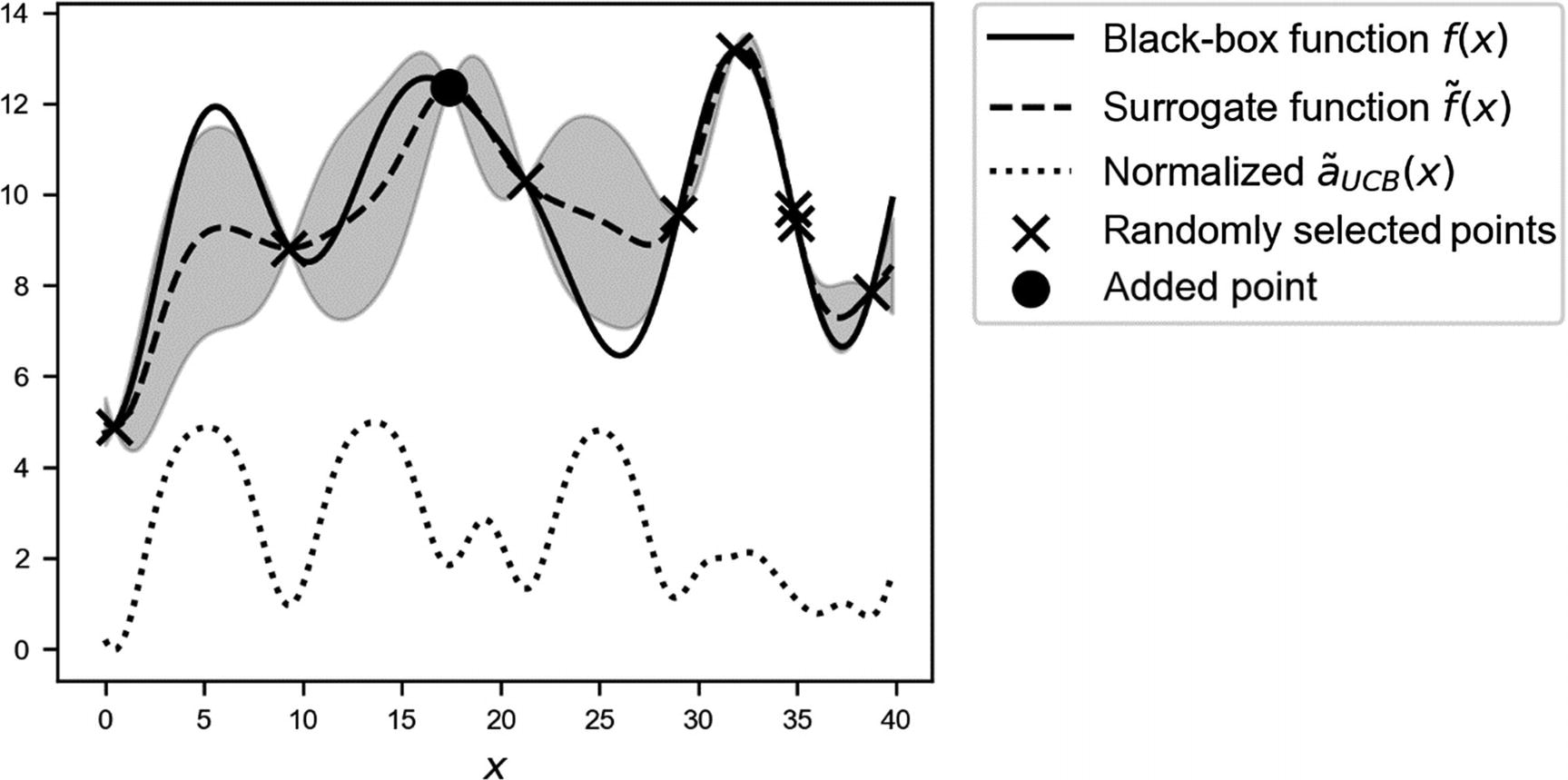
Overview of the black-box function
f(x) (solid line), the randomly selected points (marked by crosses), and the additional selected point (marked by a black circle), the surrogate function (dashed line), and the acquisition function  (dotted line), shifted to fit in the plot. The gray area is the region contained between the lines
  and
and  .
.
Overview of the black-box function
f(x) (solid line), the randomly selected points with the additional selected points (marked by crosses), the surrogate function (dashed line), and the acquisition function  (dotted line), shifted to fit in the plot. The gray area is the region contained between the lines
  and
and  .
.
The previous discussion and comparison of the behavior of the two types of acquisition functions should have made clear how, depending on what strategy you want to apply to approximate your black-box function, you should choose the right acquisition function.
Note
Different types of acquisition functions will give different strategies in approximating the black-box function. For example, aUCB(x) will add points in regions with the highest variance, while  will add points finding a balance, regulated by η, between the maximum of the surrogate function and areas with high variance.
An analysis of all the different types of acquisition functions would exceed the scope of this book. A good deal of research and reading of published papers is required to gain sufficient experience and understand how different acquisition functions work and behave.
If you want to use Bayesian optimization with your TensorFlow model, you don’t have to develop the method completely from scratch. You can try the library GPflowOpt that is described in a paper by Nicolas Knudde et al., “GPflowOpt: A Bayesian Optimization Library using TensorFlow,” available at https://goo.gl/um4LSy or arXiv.org .
Sampling on a Logarithmic Scale
0 points between 10−4 and 10−3
8 points between 10−3 and 10−2
89 points between 10−1 and 10−2
899 points between 1 and 10−1
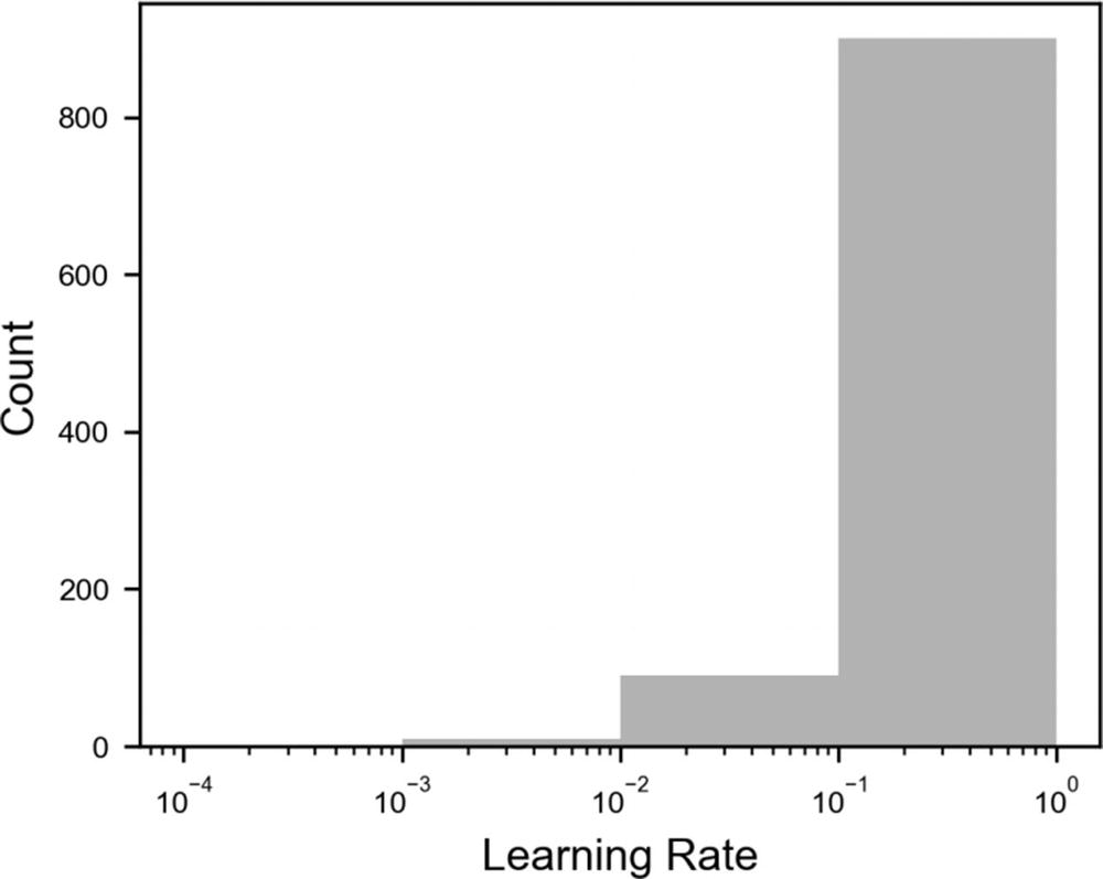
Distribution of 1000 points selected with grid search on a logarithmic x scale
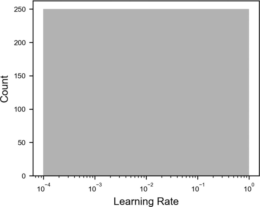
Distribution of 1000 points selected with grid search on a logarithmic x scale , with the modified selection method
Now you can see how you have the same number of points between the different powers of 10. With this simple trick, you can ensure that you also get enough points in the region of your chosen range, where, otherwise, you would get almost no points. Remember that in this example, with 1000 points, with the standard method, we get zero points between 10−3 and 10−4. This range is the most interesting for the learning rate, so you want to have enough points in this range to optimize your model. Note that the same applies to random search. It works in the exact same way.
Hyperparameter Tuning with the Zalando Dataset
To give you a concrete example of how hyperparameter tuning works, let’s apply what we have learned in a simple case. Let’s start with the data, as usual. We’ll use the Zalando dataset from Chapter 3. For a complete discussion, please refer to that chapter. Let’s quickly load and prepare the data and then discuss tuning.
and, additionally, we evaluate the accuracy on the train dataset and on the dev dataset and return the values to the caller. In this way, we can run a loop for several values of the number of neurons in the hidden layer and get the accuracies. Note, this time, that the function has an additional input parameter: number_neurons. We must pass this number to the function that builds the model.
Let’s suppose we choose the following parameters: minibatch size = 50, we train for 100 epochs, the learning rate =0.00 , and we build our model with 15 neurons in the hidden layer.
Overview of the Accuaracy on the Train and Test Datasets for a Different Number of Neurons
Number of Neurons | Accuracy on the Train Dataset | Accuracy on the Test Dataset |
|---|---|---|
1 | 0.201383 | 0.2042 |
5 | 0.639417 | 0.6377 |
10 | 0.639183 | 0.6348 |
15 | 0.687183 | 0.6815 |
25 | 0.690917 | 0.6917 |
30 | 0.6965 | 0.6887 |
50 | 0.73665 | 0.7369 |
150 | 0.78545 | 0.7848 |
300 | 0.806267 | 0.8067 |
1000 | 0.828117 | 0.8316 |
3000 | 0.8468 | 0.8416 |
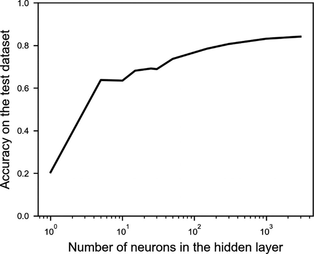
Accuracy on the test dataset vs. the number of neurons in the hidden layer
Number of neurons: Between 35 and 60
Learning rate: We will use the search on the logarithmic scale between 10−1 and 10−3.
Mini-batch size: Between 20 and 80
Number of epochs: Between 40 and 100
If you run this code, you will get a few combinations that end up in nan, and, therefore, it gets you an accuracy of 0.1 (basically random, because we have ten classes) and a few good combinations. You will find that the combinations with 41 epochs, 41 neurons in each layer, a learning rate of 0.0286, and a mini-batch size of 61 gives you an accuracy on the dev dataset of 0.86. Not bad, considering that this run took 2.5 minutes, so 14 times faster than the model with 1 layer and 3000 neurons and 6% better. Our naive initial test gave us an accuracy of 0.75, so with hyperparameter tuning, we got 11% better than our initial guess. Eleven percent increased accuracy in deep learning is an incredible result. Even 1% or 2% better is considered a great result, normally. What we did should give you an idea of how powerful hyperparameter tuning can be, if done properly. Keep in mind that you should spend quite some time doing it, thinking especially about how to do it.
Note
Always think about how you want to do your hyperparameter tuning, and use your experience, or ask for help from someone with experience. It is useless to invest time and resources to try combinations of parameters that you know will not work. For example, it is better to spend time testing learning rates that are very small than to test learning rates around one. Remember that every training round of your network will cost time, even if the results are not useful!
The point of this last section is not to get the best model possible but to give you an idea of how the tuning process may work. You could continue, trying different optimizers (for example Adam), considering wider ranges for the parameters, more parameter combinations, and so on.
A Quick Note on the Radial Basis Function

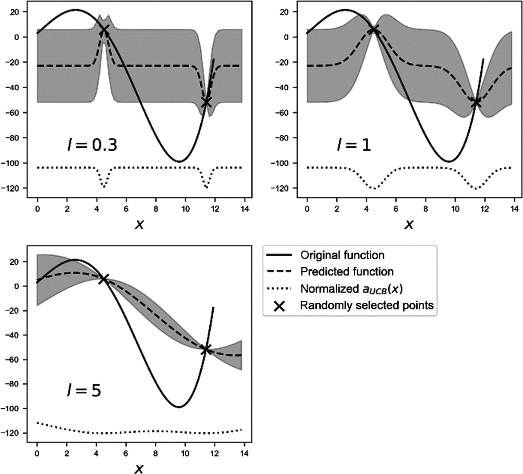
Effect of changing the parameter l in the radial basis function
Usually, it is good practice to avoid values for l that are too small or too big, to be able to have a variance that varies in a smooth way between known points, as in Figure 7-27, for l = 1. Having a very small l will make the variance between points almost constant and, therefore, make the algorithm almost always choose the middle point between points, as you can see from the acquisition function. Choosing a big l will make the variance small and, therefore, with some acquisition functions, difficult to use. As you can see for l = 5 in Figure 7-27, the acquisition function is almost constant. Typical values that are used are around 1 or 2.