11

Understanding Common Industry Challenges and Solutions

The use of ML in healthcare and life sciences can have a transformational impact on the industry. It can help find a cure for incurable diseases, prevent the next pandemic, and help healthcare professionals become more efficient at providing care. All of this helps uplift an entire population with a better quality of life and timely care. However, there are some challenges in applying ML to the healthcare and life sciences industry. Healthcare data is extremely private, requiring the highest levels of security. This prevents open sharing and collaboration among researchers to advance this field, getting in the way of innovation. There are also a variety of regulations in place that make it difficult for practical ML applications to be readily used in mission-critical workloads in the industry. Moreover, as ML models become better, they also become more complex. Neural networks (NNs) that have known to be state-of-the-art (SOTA) are usually made of extremely complicated architectures and may contain billions of parameters. This makes it extremely difficult to understand why the model is predicting the way it is. Without a good understanding of this, we are looking at a “black box” that predicts an output without ensuring whether it’s fair or transparent. This is a deterrent for adoption in the healthcare and life sciences industry, which promotes transparency and reporting to regulatory bodies.

However, not all is lost. While there are still many challenges, there are a good number of success stories around the application of ML to healthcare and life sciences workloads. For example, we have seen both Pfizer-BioNTech and Moderna develop an entirely new vaccine for the novel coronavirus in record time by applying ML to different stages of the drug discovery and clinical trial pipeline. We have seen companies such as Philips and GE Healthcare that have revolutionized medical imaging by using computer vision (CV) models on their equipment. We also see numerous examples of start-ups being formed with the goal of curing cancer by utilizing ML models that can find a variety of characteristics from genomic and proteomic data. All these examples prove that there are ways in which you can apply ML technology successfully in this industry. This is happening by utilizing workarounds and solutions that enable you to address and meet these challenges head-on. It is a matter of knowing how to address them and finding the best alternative by balancing complexity, transparency, and usefulness.

In this chapter, we will look at some of the common challenges that come in the way of applying ML to workloads in the healthcare and life sciences industry. We will then look at some ways to address those challenges by understanding workarounds and solutions. We will get introduced to new features of SageMaker, SageMaker Clarify and SageMaker Model Monitor, that help you create fair and transparent AI models for healthcare and life sciences workloads. Lastly, we will use this feature to get a better understanding of an ML model that predicts healthcare coverage amounts for patients across different demographics.

Here are the main topics we will cover in this chapter:

• Understanding challenges with implementing ML in healthcare and life sciences
• Understanding solution options for solving these challenges
• Introducing SageMaker Clarify and Model Monitor
• Detecting bias and explaining model predictions for healthcare coverage amounts
• Viewing bias and explainability reports in SageMaker Studio

Technical requirements

You need to complete the following technical requirements before building the example implementation at the end of this chapter:

1. Complete the steps to set up the prerequisites for Amazon SageMaker, as described here: https://docs.aws.amazon.com/sagemaker/latest/dg/gs-set-up.html.
2. Onboard to SageMaker Domain using Quick setup, as described here: https://docs.aws.amazon.com/sagemaker/latest/dg/onboard-quick-start.html.

Note

If you have already onboarded a SageMaker Domain from a previous exercise, you do not need to perform step 2 again.

3. Once you are in the SageMaker Studio interface, click on File | New | Terminal.
4. Once in the terminal, type the following commands:

   git clone https://github.com/PacktPublishing/Applied-Machine-Learning-for-Healthcare-and-Life-Sciences-using-AWS.git

You should now see a folder named Applied-Machine-Learning-for-Healthcare-and-Life-Sciences-using-AWS.

Note

If you have already cloned the repository in a previous exercise, you should already have this folder. You do not need to do step 4 again.

5. Familiarize yourself with the SageMaker Studio UI components, as described here: https://docs.aws.amazon.com/sagemaker/latest/dg/studio-ui.html.

Once you have completed these steps, you should be all set to execute the steps in the example implementation in the last section of this chapter.

Understanding challenges with implementing ML in healthcare and life sciences

We have seen multiple examples of the use of ML in healthcare and life sciences. These include use cases for providers, payers, genomics, drug discovery, and many more. While we have shown how ML can solve some of the biggest challenges that the healthcare industry is facing, implementing it at scale for healthcare and life sciences workloads has some inherent challenges. Let us now review some of those challenges in more detail.

Healthcare and life sciences regulations

Healthcare and life sciences is a highly regulated industry. There are laws that protect a patient’s health information and ensure the security and privacy of healthcare systems. There are some laws that are specific to countries that the patients reside in, and any entity that interacts with data for those patients needs to comply with those rules. Let’s look at some examples of such regulations:

• Health Insurance Portability and Accountability Act (HIPAA): In the US, the Department of Health and Human Services (HHS) created a set of privacy rules under HIPAA that standardized the protection of personally identifiable health information also known as protected health information (PHI). As part of these standards, it included provisions to allow individuals to understand and control how their health information is used. This applies to all covered entities as defined in HIPAA. They include healthcare providers, health plans, healthcare clearinghouses, and business associates.
• Health Information Technology for Economic and Clinical Health (HITECH): HITECH is another regulation specific to US healthcare. HITECH was created to increase the adoption of the electronic health record (EHR) system. It includes provisions for grants and training for employees who are required to support health IT infrastructure. It also includes requirements for data breach notifications and increased penalties for HIPAA violations. As a matter of fact, HIPAA and HITECH are closely related in the way they reinforce each other. For example, under HITECH, the system requirements that were put in place ensure that they do not violate any HIPAA laws.
• General Data Protection Regulation (GDPR): GDPR is a European law that was implemented in 2018. It intends to harmonize data protection and privacy laws across the European Union (EU). It applies to any organization (operating within or outside of the EU) that processes and accesses the personal data (personally identifiable information, or PII) of anyone in the EU and aims to create consistency across EU member states on how personal data can be processed, used, and exchanged securely.
• GxP: GxP compliance broadly refers to good practices for life sciences organizations that manufacture medical products such as drugs, medical devices, and medical software applications. It can have variations depending on the area of life sciences that it’s applied in. For example, you can have Good Manufacturing Practices (GMPs), Good Laboratory Practices (GLPs), and Good Clinical Practices (GCPs). The goal of all GxP compliance variations is to ensure safety and quality through the use of validated systems that operate per their intended use.

Let us now look at some security- and privacy-related requirements when it comes to healthcare and life sciences workloads.

Security and privacy

Healthcare data needs to be handled with care to ensure there are no violations of any of the regulatory guidelines such as HIPAA or GDPR. There are huge penalties for organizations that do not comply. For example, the total fines for healthcare organizations that reported HIPAA violations between 2017 and 2020 were approximately USD $80 million. Moreover, the laws require you to report violations of data breaches in a timely manner to the public. This creates further embarrassment for the organizations concerned and leads to a lack of trust and negative consumer sentiment. There is no doubt that it is absolutely essential for healthcare organizations to adhere to these regulations by keeping security and privacy as an integral part of their architecture. The rules are carefully thought out and created to protect patients and keep them and their data safe.

ML is no exception when it comes to implementing security and privacy. ML data needs to be properly secured and anonymized. It needs to be access-controlled so that only authorized people or systems have access to it. The environment in which the model is trained and hosted needs to have appropriate security controls in place so that it cannot be breached. All of these are essential steps that may sometimes slow down the pace of the adoption of ML in healthcare. Nonetheless, the risk of not having these measures in place outweighs the reward that any innovation could bring.

Bias and transparency in ML

Another challenge for implementing ML technology in healthcare and life sciences workflows is the emphasis on fairness. A model that predicts a positive outcome for one demographic more often than another is said to be biased toward that demographic and cannot be considered fair. In healthcare, a biased model can be detrimental in a variety of scenarios. For example, a claims adjudication model can be biased toward approving claims for a certain gender or ethnicity more often than others. This provides better healthcare coverage for a certain group of people compared to others. We are all working toward creating a world where health equity is prioritized. This means healthcare should be available to all and should provide equal benefits for everyone. An unfair model goes against this principle. As a result, when building models for healthcare use cases, data scientists should take into account the necessary steps that ensure fairness in model predictions.

Reproducibility and generalizability of ML models

Another challenge for the adoption of ML in healthcare is the concept of generalizability. This essentially underscores the importance of the model results being reproducible across different samples of real-world data. It happens very often that we see a model that performs really well in research environments on specific test datasets but does not retain the same performance in real-world scenarios. This may be for a variety of reasons. One common reason is that the data on which the model is trained and evaluated does not mimic real-world behavior. It may also be biased toward one group or class.

Now that we have an understanding of some of the common challenges that organizations face in the adoption of ML in healthcare and life sciences workflows, let us dive into some solutions that may help address these challenges.

Understanding options for solving these challenges

While there are known challenges, there are ways organizations can successfully adopt ML in healthcare and life sciences workloads. One important factor to consider is at what stage in the workflow you apply ML. While there have been improvements to the technology, it is not a replacement for a trained medical professional. It cannot replace the practical experience and knowledge gathered through years of practice and training. However, technology can help make medical professionals more efficient at what they do. For example, instead of relying on an ML model to make diagnostic decisions for a patient, it can be used to recommend a diagnosis to a healthcare provider and let them make a final decision. It can act as a tool for them to search through a variety of case reports and medical history information that will help them in their decision-making process. The medical professional is still in control while getting a superpower that has the ability to automate mundane and repeatable tasks and also augment the practical experience of a provider instead of replacing it. Let us now look at some common technical methods to consider in your ML pipeline to make it suitable for healthcare and life sciences workloads.

Encrypting and anonymizing your data

Data encryption is a common way to protect sensitive information. It involves transforming your original data into another form or code that is impossible to understand or decipher. The only way to retrieve the original plain text information is via decryption, which reverses the operation. To achieve this, you must have access to the encryption/decryption key, which is a unique secret key. No one without access to this secret key can access the underlying data, hence making it useless.

Utilizing encryption algorithms to transform your sensitive healthcare information helps keep the data safe. The customers need to just keep the secret key secure instead of a whole database, which makes the process much more manageable and reduces the risk involved. There are some things to keep in mind, though. Firstly, using these algorithms involves extra processing, both while encrypting and decrypting. This introduces more compute overhead on your systems. Applications that rely on reading and displaying encrypted data may perform sluggishly and impact user experience. Moreover, there is a risk of hackers breaking encryption keys and getting access to sensitive information if they are too simple. Hackers rely on trial and error and run software that can generate multiple permutations and combinations until they find the right one. This pushes organizations to create more complicated and lengthy keys, which in turn adds to the processing overhead. Therefore, it is important to come up with the correct encryption setup for your data, both in transit and at rest. Understand the compute overhead, plan for it, and ensure you have enough capacity for the types of queries you run on your encrypted data.

Another way to de-sensitize your data is by using anonymization. Though encryption may be considered a type of anonymization technique, data anonymization involves methods to erase sensitive fields containing personally identifiable data from your datasets. One common way of data anonymization is data masking, which involves removing or masking sensitive fields from your dataset. You can also generate synthetic versions of the original data by utilizing statistical models that can generate a representative set similar to the original dataset. The obvious consideration here is the method of anonymization. While methods such as data masking and erasing are easy to implement, they may remove important information from the dataset that can be critical to the performance of the downstream analytics or ML models. Moreover, removing all sensitive information from the data affects its usability for personalization or recommendations. This can affect end-user experience and engagement. Security should always be the top priority for any healthcare organization, and striking a balance between technical complexity and user experience and convenience is a key aspect when deciding between data anonymization and encryption.

Explainability and bias detection

The next consideration for implementing ML models in healthcare workflows is how open and transparent the underlying algorithm is. Are we able to understand why a model is predicting a particular output? Do we have control over the parameters to influence its prediction when we choose to do so? These are the questions that model explainability attempts to answer. The key to explaining model behavior is to interpret it. Model interpretation helps increase trust in the model and is especially critical in healthcare and life sciences. It also helps us understand whether the model is biased toward a particular class or demographic, enabling us to take corrective action when needed. This can be due to a bias in the training dataset or in the trained model. The more complicated a model is, the more difficult it is to interpret and explain its output. For example, in NNs that consist of multiple interconnected layers that transform the input data, it is difficult to understand how the input data impacts the final prediction. However, a single-layer regression model is far easier to understand and explain. Hence, it is important to balance SOTA with simplicity. It is not always necessary to use a complicated NN if you can achieve acceptable levels of performance from a simple model. Similarly, it may not always be necessary to explain model behavior if the use case it’s being implemented for is not mission-critical.

Model explanations can be generated at a local or a global level. Local explanations attempt to explain the prediction from a model for a single instance in the data. A way to generate a local explanation for your model is to utilize Local Interpretable Model-Agnostic Explanations (LIME). LIME provides local explanations for your model by building surrogate models using permutations of feature values of a single dataset and observing its overall impact on the model. To know more about LIME, visit the following link: https://homes.cs.washington.edu/~marcotcr/blog/lime/. Another common technique for generating local explanations is by using SHapley Additive exPlanations (SHAP). The method relies on the computation of Shapley values that represents the feature contribution for each feature toward a given prediction. To learn more about SHAP, visit the following link: https://shap.readthedocs.io/en/latest/index.html. Global explanations are useful to understand the model behavior on the entire dataset to get an overall view of the factors that influence model prediction. SHAP can also be used to explain model predictions at a global level by computing feature importance values over the entire dataset and taking an average for it. Or, you can use a technique called permutation importance. This method selectively replaces features with noise and computes the model performance to adjudicate how much impact the particular feature has in overall predictions.

Building reproducible ML pipelines

As ML gets more integrated with regular production workflows, it is important to get consistent results from the model under similar input conditions. However, model outputs may change over a period of time as the model and data evolve. This could be for a variety of reasons, such as a change in business rules that influence real-world data. This is commonly referred to as model drift in ML. As you may recall, ML is an iterative process, and the model results are a probabilistic determination of the most likely outcome. This introduces a new problem of reproducibility in ML. A model or a pipeline is said to be reproducible if its results can be recreated with the given assumptions and features. It is an important factor for GxP compliance, which requires validating a system for its intended use. There are various factors that may influence inconsistent model outputs; it mostly has to do with how the model is trained. Retraining a model with a different dataset or a different set of features will most likely influence the model output. It can also be influenced by your choice of training algorithm and the associated hyperparameters.

Versioning is a key factor in model reproducibility. Versioning each step of the ML pipeline will help ensure there are no variations between them. For example, the training data, feature engineering script, training script, model, and deployed endpoint should all be versioned for each variation. You should be able to associate a version of the training dataset with a version of the feature engineering script, a version of a training script, and so on. You should then version this entire setup as a pipeline. The pipeline allows you to create traceability between each step in the pipeline and maintain it as a separate artifact. Another aspect that could influence model output variation is the compute environment on which the pipeline is run. Depending on the level of control you need on this aspect, you may choose to create a virtual environment or a container for running your ML model pipeline. By utilizing these methods, you should be able to create a traceable and reproducible ML model pipeline that runs in a controlled environment, reducing the chances of inconsistency across multiple model outputs.

Auditability and review

Auditability is key for a transparent ML model pipeline. An ideal pipeline logs each step that might need to be analyzed. Auditing may be needed to fulfill regulatory requirements, or it may also be needed to debug an issue in the model pipeline. For auditing to occur, you need to ensure that there is centralized logging set up for your ML pipeline. This logging platform is like a central hub where model pipelines can send logs. The logging platform then aggregates these logs and makes them available for end users who have permission to view them. A sophisticated logging platform also supports monitoring of real-time events and generates alerts when a certain condition is fulfilled. Using logging and monitoring together helps prevent or fix issues with your model pipeline. Moreover, the logging platform is able to aggregate logs from multiple jobs and provide log analytics for further insights across your entire ML environment. You can automatically generate audit reports for your versioned pipeline and submit them for regulatory reviews. This saves precious time for both the regulators and your organization.

While logging and monitoring are absolutely essential for establishing trust and transparency in ML pipelines, they may sometimes not be enough by themselves. Sometimes, you do need the help of humans to validate model output and override those predictions if needed. In ML, this is referred to as a human-in-the-loop pipeline. It essentially involves sending model predictions to humans with subject-matter expertise to determine whether the model is predicting correctly. If not, they can override the model predictions with the correct output before sending the output downstream. This intervention by humans can also be enabled for selected predictions. Models can generate a confidence score for each prediction that can be used as a threshold for human intervention. Predictions with high confidence scores do not require validation by humans and can be trusted. The ones with confidence scores below a certain threshold can be selectively routed to humans for validation. This ensures only valid cases are being sent for human review instead of increasing human dependency on all predictions. As more and more data is generated with validated output, it can be fed back to the training job to train a new version of the model. Over multiple training cycles, the model can learn the new labels and begin predicting more accurately, requiring even lesser dependency on humans. This type of construct in ML is known as an active learning pipeline.

These are some common solutions available to you when you think about utilizing ML in healthcare and life sciences workflows. While there is no single solution that fits all use cases and requirements, utilizing the options discussed in this section will help ensure that you are following all the best practices in your model pipeline. Let us now learn about two new features of SageMaker, SageMaker Clarify and Model Monitor, and see how they can help you detect bias, explain model results, and monitor models deployed in production.

Introducing SageMaker Clarify and Model Monitor

SageMaker Clarify provides you with greater visibility into your data and the model it is used to train. Before we begin using a dataset for training, it is important to understand whether there is any bias in the dataset. A biased dataset can influence the prediction behavior of the model. For instance, if a model is trained on a dataset that only has records for older individuals, it will be less accurate when applied to predict outcomes for younger individuals. SageMaker Clarify also allows you to explain your model by showing you reports of which attributes are influencing the model’s prediction behavior. Once the model is deployed, it needs to be monitored for changes in behavior over time as real-world data changes. This is done using SageMaker Model Monitor, which alerts you if there is a shift in the feature importance in the real-world data.

Let us now look at SageMaker Clarify and Model Monitor in more detail.

Detecting bias using SageMaker Clarify

SageMaker Clarify uses a special processing container to compute bias in your dataset before you train your model with it. These are called pre-training bias metrics. It also computes bias metrics in the model predictions after training. These are known as post-training bias metrics. Both of these metrics are computed using SageMaker Processing jobs. You have the option to use Spark to execute processing jobs, which is especially useful for large datasets. SageMaker Clarify automatically uses Spark-based distributed computing to execute processing jobs when you provide an instance count greater than 1. The processing job makes use of the SageMaker Clarify container and takes specific configuration inputs to compute these metrics. The reported metrics can then be visualized on the SageMaker Studio interface or downloaded locally for post-processing or integration with third-party applications. Let us now look at some of the common pre-training and post-training bias metrics that SageMaker Clarify computes for you.

Pre-training bias metrics

Pre-training bias metrics attempt to understand the data distributions for all features in the training data and how true they are to the real world. Here are some examples of metrics that help us determine this:

• Class Imbalance (CI): CI occurs when a certain category is over- or under-represented in the training dataset. An imbalanced dataset may result in model predictions being biased toward the over-expressed class. This is not desirable, especially if it doesn’t represent real-world data distribution.
• Difference in Proportions in Labels (DPL): This metric tries to determine whether the labels of target classes are properly distributed among particular groups in the training dataset. In the case of binary classification, it determines the proportion of positive labels in one group compared to the proportion of positive labels in another group. It helps us measure whether there is an equal distribution of the positive class within each group in the training dataset.
• Kullback-Leibler (KL) divergence: The KL divergence metric measures how different the probability distribution of labels of one class is from another. It’s a measure of distance (divergence) between one probability distribution and another.
• Conditional Demographic Disparity in Labels (CDDL): This metric determines the disparity in label distribution within subgroups of training data. It measures whether the positive class and negative class are equally distributed within each subgroup. This helps us determine whether one subgroup (say, people belonging to an age group of 20–30 years) has more positive classes (say, hospital readmissions) than another subgroup (people belonging to a different age group).

These are just four of the most common pre-training metrics that SageMaker Clarify computes for you. For a full list of pre-training metrics, refer to the white paper at the following link: https://pages.awscloud.com/rs/112-TZM-766/images/Amazon.AI.Fairness.and.Explainability.Whitepaper.pdf.

Post-training bias metrics

SageMaker Clarify provides 11 post-training bias metrics for models and data that help you determine whether the model predictions are fair and representative of real-world outcomes. Users have a choice to use a subset of these metrics depending on the use case they are trying to implement. Moreover, the definition of fairness for a model also differs from use case to use case, and so does the computation of metrics that determine the concept of fairness for that particular model. In a lot of cases, human intervention and stakeholder involvement are needed to ensure correct metrics are being tracked to measure model fairness and bias. Let us now look at some of the common post-training metrics that SageMaker Clarify can compute for us:

• Difference in Positive Proportions in Predicted Labels (DPPL): This metric measures the difference between the positive predictions in one group versus another group. For example, if there are two age groups in the inference data for which you need to predict hospital readmissions, DPPL measures whether one age group is predicted to have more readmissions than the other.
• Difference in Conditional Outcome (DCO): This metric measures the actual values for different groups of people in the inference dataset, compared to the predicted values. For example, let’s assume there are two groups of people in the inference dataset: male and female. The model is trying to predict whether their health insurance claim would be accepted or rejected. This metric looks at the actual approved claims compared to rejected applications for both male and female applicants in the training dataset and compares it with the predicted values from the model in the inference dataset.
• Recall Difference (RD): Recall is a measure of a model’s ability to predict a positive outcome in cases that are actually positive. RD measures the difference between the recall values of multiple groups with the inference data. If the recall is higher for one group of people in the inference dataset compared to another group, the model may be biased toward the first group.
• Difference in Label Rates (DLR): Label rate is a measure of the true positive versus predicted positive (label acceptance rate) or a measure of true negative versus predicted negative (label rejection rate). The difference between this measure across different groups in the dataset is captured by the DLR metric.

These are just four of the common metrics that SageMaker Clarify computes for you post-training. For a full list of these metrics and their details, refer to the SageMaker Clarify post-training metrics list here: https://docs.aws.amazon.com/sagemaker/latest/dg/clarify-measure-post-training-bias.html.

SageMaker Clarify also helps explain our model prediction behavior by generating an importance report for the features. Let us now look at model explainability with SageMaker Clarify in more detail.

Explaining model predictions with SageMaker Clarify

A model explanation is essential for building trust and understanding what is influencing a model to predict in a certain way. For example, it lets you understand why a particular patient might be at a higher risk of congestive heart failure than another. Explainability builds trust in the model by making it more transparent instead of treating it as a black box. SageMaker Clarify generates feature importance for the model using Shapley values. This helps determine the contribution of each feature in the final prediction. Shapley values are standard for the determination of feature importance and compute the effects of each feature in combination with another. SageMaker Clarify uses an optimized implementation of the Kernel SHAP algorithm. To learn more about SHAP, you can refer to the following link: https://en.wikipedia.org/wiki/Shapley_value.

SageMaker Clarify also allows you to generate a partial dependence plot (PDP) for your model. It shows the dependence of the predicted target on a set of input features of interest. You can configure inputs for the PDP using a JSON file. The results of the analysis are stored in the analysis.json file and contain the information needed to generate these plots. You can then generate a plot yourself or visualize it in the SageMaker Studio interface.

In addition to Shapley values and PDP analysis, SageMaker Clarify can also generate heatmaps for explaining predictions on image datasets. The heatmaps explain how CV models classify images and detect objects in those images. In the case of image classification, the explanations consist of images, with each image showing a heatmap of the relevant pixels involved in the prediction. In the case of object detection, SageMaker Clarify uses Shapley values to determine the contribution of each feature in the model prediction. This is represented as a heatmap that shows how important each of the features in the image scene was for the detection of the object.

Finally, SageMaker Clarify can help explain prediction behavior for natural language processing (NLP) models with classification and regression tasks. In this case, the explanations help us understand which sections of the text are the most important for the predictions made by the model. You can define the granularity of the explanations by providing the length of the text segment (such as phrases, sentences, or paragraphs). This can also extend to multimodal datasets where you have text, categorical, and numerical values in the input data.

Now that we have an idea of how SageMaker Clarify helps in bias detection and explaining model predictions, let us look at how we can monitor the performance of the models once they are deployed using real-world inference data. This is enabled using SageMaker Model Monitor.

Monitoring models with SageMaker Model Monitor

SageMaker Model Monitor allows you to continuously monitor model quality and data quality for a deployed model. It can notify you if there are deviations in data metrics or model metrics, allowing you to perform corrective actions such as retraining the model. The process of monitoring models with SageMaker Model Monitor involves four essential steps:

1. Enable the endpoint to capture data from incoming requests.
2. Create a baseline from the training dataset.
3. Create a monitoring schedule.
4. Inspect the monitoring metrics in the monitoring reports.

We will go through these steps during the exercise at the end of this chapter.

In addition, you can also enable data quality and model quality monitoring in SageMaker Studio and visualize the result on the SageMaker Studio interface. Let us now look at the details of how to set up a data quality and a model quality monitoring job on SageMaker Model Monitor.

Setting up data quality monitoring

SageMaker Model Monitor can detect drift in the dataset by comparing it against a baseline. Usually, the training data is a good baseline to compare against. SageMaker Model Monitor can then suggest a set of baseline constraints and generate statistics to explore the data. These are available inside statistics.json and constraints.json files. You can also enable SageMaker Model Monitor to directly emit data metrics to CloudWatch metrics. This allows you to generate alerts from CloudWatch if there is a violation in any of the constraints you are monitoring.

Setting up model quality monitoring

SageMaker Model Monitor can monitor the performance of a model by comparing the predicted value with the actual ground truth. It then evaluates metrics depending on the type of problem at hand. The steps to configure model quality monitoring are the same as the steps for data quality monitoring, except for an additional step to merge the ground-truth labels with the predictions. To ingest ground-truth labels, you need to periodically label the data captured by the model endpoint and upload it to a Simple Storage Service (S3) location from where SageMaker Model Monitor can read it. Moreover, there needs to be a unique identifier (UID) in the ground-truth records and a unique path on S3 where the ground truth is stored so that it can be used by SageMaker Model Monitor to access it.

It’s important to note that SageMaker Model Monitor also integrates with SageMaker Clarify to enable bias-drift detection and feature attribution-drift detection on deployed models. This provides you the ability to carry out these monitoring operations on real-time data that is captured from an endpoint invocation. You can also define a monitoring schedule and a time window for when you want to monitor the deployed models.

SageMaker Clarify and Model Monitor provide you with the ability to create fair and explainable models that you can monitor in real time. Let us now use SageMaker Clarify to create a bias detection workflow and explain model predictions.

Detecting bias and explaining model predictions for healthcare coverage amounts

Bias in ML models built to predict critical healthcare metrics can erode trust in this technology and prevent large-scale adoption. In this exercise, we will start with some sample data about healthcare coverage and expenses for about 1,000 patients belonging to different demographics. We will then train a model to predict how much the coverage-to-expense ratio is for patients in different demographics. Following that, we will use SageMaker Clarify to generate bias metrics on our training data and trained model. We will also generate explanations of our prediction to understand why the model is predicting the way it is. Let’s begin by acquiring the dataset for this exercise.

Acquiring the dataset

The dataset used in this exercise is synthetically generated using Synthea, an open source synthetic patient generator. To learn more about Synthea, you can visit the following link: https://synthetichealth.github.io/synthea/. Follow the next steps:

1. We use a sample dataset from Synthea for this exercise that can be downloaded from the following link: https://synthetichealth.github.io/synthea-sample-data/downloads/synthea_sample_data_csv_apr2020.zip.
2. The link will download a ZIP file. Unzip the file, which will create a directory called csv with multiple CSV files within it.

We will use only the patients.csv file for this exercise.

Running the Jupyter notebooks

The notebook for this exercise is saved on GitHub here:

https://github.com/PacktPublishing/Applied-Machine-Learning-for-Healthcare-and-Life-Sciences-using-AWS/blob/main/chapter-11/bias_detection_explainability.ipynb

The repository was cloned as part of the steps in the Technical requirements section. You can access the notebook from GitHub by following these steps:

1. Open the SageMaker Studio interface.
2. Navigate to the Applied-Machine-Learning-for-Healthcare-and-Life-Sciences-using-AWS/chapter-11/ path. You should see a file named bias_detection_explainability.ipynb.
3. Select New Folder at the top of the folder navigation pane in SageMaker Studio, as shown in the following screenshot:

Figure 11.1 – SageMaker Studio UI showing the New Folder button

4. Name the folder data. Next, click the Upload Files icon on the top of the navigation pane in SageMaker Studio, as shown in the following screenshot:

Figure 11.2 – SageMaker Studio UI showing the Upload Files button

5. Upload the patients.csv and salesdaily.csv files that you downloaded earlier.
6. Go back one folder to Chapter-11 and click on the bias_detection_explainability.ipynb file. This will open the Jupyter notebook. Follow the instructions in the notebook to complete this step.

Let us now look at the steps to visualize the reports generated in this step in SageMaker Studio. After running the notebook, you can proceed with the next section to visualize the report on SageMaker Studio.

Viewing bias and explainability reports in SageMaker Studio

After completing the steps in the preceding section, SageMaker Clarify creates two reports for you to examine. The first report allows you to look at the bias metrics for your dataset and model. The second report is the explainability report, which tells you which features are influencing the model predictions. To view the reports, follow these steps:

1. Click on SageMaker resources in the left navigation pane of SageMaker Studio. Make sure Experiments and trials is selected in the drop-down menu:

Figure 11.3 – SageMaker Studio interface showing the SageMaker resources button

2. Double-click on Unassigned trial components at the top of the list. In the next screen, you will see two trials. The first trial starts with clarify-explainability and the second starts with clarify-bias.
3. Double-click on the report starting with clarify-bias. Navigate to the Bias report tab, as shown in the following screenshot:

Figure 11.4 – SageMaker Clarify Bias report tab

4. Here, you can examine the bias report generated by SageMaker Clarify. It has a variety of metrics that are calculated for your dataset and model. You can expand each metric and read about what the scores might mean for your dataset and model. Spend some time reading about these metrics and assess whether the data we used has any bias in it. Remember to change the AGEGROUPS values using the top drop-down menu.
5. You can also view a summary of all metrics in a tabular format by clicking on the Table button in the top-right corner, as shown in the following screenshot:

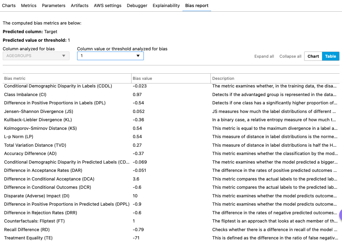
Figure 11.5 – Summary of bias metrics in SageMaker Studio

6. Next, let’s look at the explainability report. Follow steps 1 and 2 of this section to go to the screen that has the clarify-explainability trial. Double-click on it.
7. On the next screen, click on the Explainability tab at the top. This will open up the explainability report, as shown in the following screenshot:

Figure 11.6 – Explainability report in SageMaker Studio

As you can see, the AGEGROUPS feature has the most impact on the model’s prediction while the CITY feature has the least impact. You can also access the raw data in JSON used to generate this report and export the report into a PDF for easy sharing. This concludes the exercise.

Summary

In this chapter, we looked at some of the challenges that technologists face when implementing ML workflows in the healthcare and life sciences industry. These include regulatory challenges, security and privacy, and ensuring fairness and generalizability. We also looked at ways that organizations are addressing those challenges. We then learned about SageMaker Clarify and Model Monitor, and how they ensure fairness and provide explainability for ML models. Finally, we used SageMaker Clarify to create a bias and explainability report for a model that predicts healthcare coverage amounts.

In Chapter 12, Understanding Current Industry Trends and Future Applications, we will paint a picture of what to expect in the future for AI in healthcare. We will look at some newer innovations in this field and conclude by summarizing some trends.