5

Implementing Machine Learning for Healthcare Payors

Health insurance is an integral part of a person’s well-being and financial security. Unlike countries such as the UK and Canada, the US does not have a concept of universal healthcare. The majority of US residents are covered by plans from their employers who contract with private health insurance companies. Others rely on public insurance such as Medicare and Medicaid. The rising cost of healthcare has made it almost impossible for anyone to survive without health insurance. No wonder that, by the end of 2020, over 297 million people in the US had coverage for health insurance, with the number trending higher every year.

Health insurance companies, also known as healthcare payors, are organizations that cover the healthcare costs incurred by subscribers to their plan, known as payees. The payees (patients) or providers submit a claim to the payor for the costs incurred, and the payor, after doing their due diligence, pays out the amount to the beneficiary. For a fixed amount paid at regular intervals, known as a premium, the subscribers get access to coverage of healthcare costs such as preventive care visits, labs, medical procedures, and prescription drugs. The costs that they pay out of pocket and the healthcare costs that are covered depend on the health insurance plan, or simply the health plan. The health plan is a package of charges and services that the payor provides as a choice to their subscribers. Most of these health plans come with a deductible amount that needs to be paid out of pocket before the cover kicks in; the amount of the deductible is decided by the plan you pick.

In this chapter, we will look into the details of how a health insurance company processes a claim, which is the largest Operational Expense (OpEx) for a payor. We will look at the different stages of claim processing and the areas of optimizing the claim processing workflow. These optimizations are driven by ML models that can automate manual steps and find hidden patterns in claims data, from which operational decisions can be made. Then, we will become familiar with SageMaker Studio, the ML integrated development environment (IDE) from AWS, and use it to build an example model for predicting the claim amount for Medicare patients. In this chapter, we will cover the following topics:

• Introducing healthcare claims processing
• Implementing machine learning in healthcare claims processing workflows
• Introducing Amazon SageMaker Studio
• Building an ML model to predict Medicare claim amounts

Technical requirements

The following are the technical requirements that you need to complete before building the example implementation at the end of this chapter:

1. Complete the steps to set up the prerequisites for Amazon SageMaker, as described here: https://docs.aws.amazon.com/sagemaker/latest/dg/gs-set-up.html.
2. Create an S3 bucket, as described in Chapter 4, section Building a smart medical transcription application on AWS section, under the Creating an S3 bucket. If you already have an S3 bucket, you can use that instead of creating a new bucket.
3. Onboard to SageMaker Studio Domain using the quick setup, as described here: https://docs.aws.amazon.com/sagemaker/latest/dg/onboard-quick-start.html.

Note

If you have already onboarded a SageMaker Studio domain from a previous exercise, you do not need to perform step 3 again.

4. Once you are in the SageMaker Studio interface, click on File | New | Terminal.
5. Once in the terminal, type the following command:

   git clone https://github.com/PacktPublishing/Applied-Machine-Learning-for-Healthcare-and-Life-Sciences-using-AWS.git

You should now see a folder named Applied-Machine-Learning-for-Healthcare-and-Life-Sciences-using-AWS.

Note

If you have already cloned the repository in a previous exercise, you should already have this folder. You do not need to do step 5 again.

6. Familiarize yourself with the SageMaker Studio UI components: https://docs.aws.amazon.com/sagemaker/latest/dg/studio-ui.html.

Once you have completed the preceding steps, you should be all set to execute the steps in the example implementation in the final section of this chapter.

Introducing healthcare claims processing

Claims are at the heart of how money is exchanged between healthcare payors and the provider’s ecosystem. A claim decides the amount that a provider gets for the healthcare services they perform. There are multiple stages in the life cycle of a claim from the time it is submitted, adjudicated, and disbursed. This process is known as claims processing, and the associated workflow is known as a claims processing workflow.

Before we look into the details of claims processing stages, it is important to understand what a claim typically contains. The claim has some basic information about the patient in question. It has the details of the healthcare services that the patient received and the charges for those services as quoted by the provider. If the payor agrees with the charges, it pays the amount to the provider. Most of these claims are paid out by the payor directly to the provider, but there are some instances when a patient needs to be involved. The most common reason for this is the health plan that the patient is enrolled in doesn’t fully cover the cost of the healthcare service they received, in which case the provider sends an invoice for the remaining amount to the patient to be paid directly to the provider. This completes the full life cycle of the claim. The claims processing workflow consists of multiple steps that might vary from payor to payor. However, the basic workflow stages consist of some key steps that are consistent. Now, let us look at these steps of claims processing, as shown in the following diagram:

Figure 5.1 – Claims processing workflow

Now, let us describe the steps in more detail:

1. The provider submits an electronic or a paper claim to the health insurance company. Sometimes, it might be a claim submitted directly by the patients for the services they have already paid for to reimburse themselves.
2. The first step that the payors do is to check the claim for completeness and accuracy. For example, are all the mandatory fields complete, are there any typos in the claim, is the data accurate, and is the claim within the prescribed time deadline? If not, the claim is sent back for corrections and resubmission.
3. The next step is to extract services and member details. The member details are used to verify the status of the member with the health insurance company and also if they are covered for the services being claimed per the health plan they are enrolled in. If not, the claim is denied and sent back with reasons for denial.
4. The next step is to find out if the claim is per the guidelines. These are broad-ranging guidelines to check things such as whether the services are needed in the context of the patient’s history, are the services safe for the patient, and whether the service will improve the patient’s condition. This is to ensure that the patients are not billed for the care they don’t need. If not, the adjudicator sends the claim back to get more data and clarification about the claim or the associated amounts.
5. The next step is to find out if there is a risk of fraud in the claim using a set of predefined criteria. If the claim is determined to be fraudulent, it is denied.
6. Finally, if all checks pass, the claim amount is paid and the subscriber is sent a statement, known as the explanation of benefits for their records.

Now that we have a good understanding of the claims processing workflow, let us look at how we can optimize it by applying ML at various stages of the workflow.

Implementing ML in healthcare claims processing workflows

Health insurance companies make money by collecting premiums from their subscribers. Hence, the more subscribers they have, the better it is for their business. However, the larger the subscriber base, the greater the number of claims to process. Not to mention the complexities as a result of managing large health plans and choices. These introduce bottlenecks in claim processing. The good news is that most of the steps in claims processing, as highlighted in the previous section, are repetitive and manual. This provides us with the opportunity to automate some of these tasks using ML. Now, let us look at a few examples of the application of ML in claims processing:

• Extracting information from claims: There is still a large volume of claims that get submitted as paper claims. These claims require humans to parse information from the claim forms and manually enter the details of the claims in a digital claim transaction system to be stored in a database. Moreover, the extracted information is also manually verified for accuracy and completeness. By utilizing optical character recognition (OCR) software, you can automate the extraction of information from claim forms. OCR technology is driven by computer vision models trained to extract information from specific fields, sections, pages, or tables in a claim form. The information extracted from these models is easily verifiable for completeness and accuracy using simple rules that can be programmatically run and managed. The AWS service Textract is an OCR service that allows you to extract information into PDFs and images and provides APIs that enable you to integrate Textract into a claims processing workflow.
• Checking whether the claim is per guidelines: Checking if the claim is compliant and is per guidelines requires a deeper analysis of the claim data. Usually, this is not possible using a rules-based approach and requires the application of natural language processing (NLP) algorithms on claims data. For example, one of the key steps in checking a claim’s compliance is to extract clinically relevant entities from it. A named entity recognition (NER) model can extract key entities from the claim data such as diagnoses, medications, test names, procedure names, and more, removing the need to manually extract such information. Amazon Comprehend Medical is a service that does just that. Sometimes, these entities might need to be combined with other features such as the demographic details of the patient, the provider details, and the historical information about the patient’s conditions and past claims. This combined view can provide new insights into the claim, and ML algorithms can learn from these features to check compliance with specific guidelines.
• Checking the risk of fraud: Fraud detection in healthcare claims is one of the most common use cases. It involves ingesting claim records from multiple data sources and using them to identify anomalies in these transactions. You can approach this as a supervised or unsupervised learning problem. In the supervised setting, the algorithm can learn from labeled data to classify a transaction as fraudulent. In an unsupervised setting, the algorithms can point out how much a particular transaction differs from the others and flag them as anomalous. Both these approaches are designed to remove manual intervention and lower the rate of claim denials due to fraud, which is a huge overhead for healthcare payors.
• Financial trends and budgeting: With the cost of healthcare increasing every year, healthcare payors need to regularly evaluate their plan premiums and claim amounts to make sure they are profitable. ML can identify trends and patterns in the financial data in claims and predict future forecasts and costs. This allows payors to revise plan structures and premium costs for future subscribers.

Now let us use ML to build a model to predict claim costs. Before we do that, we will dive into SageMaker Studio, a service from AWS that we will use to build the model.

Introducing Amazon SageMaker Studio

Amazon SageMaker Studio is an IDE for ML that is completely web-based and fully managed by AWS resources in the background. It provides an intuitive interface to access ML tools to build, train, deploy, monitor, and debug your ML models. It also provides studio notebooks, which have a JupyterLab interface preinstalled with popular data science libraries that allow you to begin experimenting immediately upon getting access to the studio notebooks interface. These notebooks can be scaled up or down for CPUs or GPUs depending on the workloads you want to run on them and also provides terminal access for you to install and manage third-party libraries for local runs of your experiments. Once you are done experimenting locally, you can call multiple SageMaker jobs to scale out your experiments to larger datasets and workloads that can be horizontally scaled to multiple instances instead of a single notebook environment. For example, SageMaker Processing jobs can scale out and preprocess training data for feeding into a SageMaker Training job that can then train a model on large-scale datasets. The trained model can then be deployed as a SageMaker endpoint for real-time inference via an API call. This workflow can be templatized and maintained as a pipeline using SageMaker Pipelines to make it repeatable and managed as a production MLOps pipeline.

SageMaker tools

There are multiple ML tools available for access from within the Sagemaker Studio interface that makes integrating them into your workflows easy. You can refer to the complete list of features related to Sagemaker Studio in the SageMaker Studio developer guide here: https://docs.aws.amazon.com/sagemaker/latest/dg/studio.html

In this chapter, we will touch upon two aspects of the SageMaker Studio IDE, which we will use in the example implementation in the next section, SageMaker Data Wrangler and SageMaker Studio notebooks.

SageMaker Data Wrangler

SageMaker Data Wrangler allows you to create preprocessing data workflows for your downstream ML training jobs. ML algorithms need data to exist in a certain format before you can start training. SageMaker Data Wrangler provides a visual workflow building interface known as a data flow to design and manage different transformations to your data as you make it suitable for ML algorithms. You can then choose to analyze your transformed data or export the data into S3. Additionally, you have options to templatize the processing using a processing job or a SageMaker pipeline. Let us look at some of these features in more detail.

Importing your data

You can import data into data wrangler from a variety of AWS sources such as S3, Athena, and Redshift. You can also import data into Data Wrangler from non-AWS sources such as Data Bricks (using a JDBC driver) and Snowflake. Depending on the choice of your data source, you can provide the required parameters for Data Wrangler to authenticate and pull data from those sources.

Once imported, the dataset automatically appears in the data flow screen as the starting point of a data flow. Data Wrangler samples the data in each column of your dataset and infers the data types for them. You can change these default datatypes by going to the data types step in your data flow and choosing Edit data types. Additionally, Data Wrangler maintains a backup of the data imported from Athena and Redshift in the default S3 bucket that SageMaker creates for you. This bucket name is formatted as a sagemaker-region-account number. Once imported, you are now ready to transform and analyze your data.

Transforming and analyzing your data

The Data Wrangler data flow screen allows you to join multiple datasets together. You can generate insights from the joined dataset by generating a data quality and insights report. The report provides important information such as missing values and outliers in your dataset, which, in turn, allows you to choose the right transformations to apply to your data. Additionally, you can choose a target column in your dataset and create a quick model to determine whether you have a good baseline upon which you would want to improve. It also gives you feature importance and column statistics for the features. These are important insights to have at the beginning of the ML life cycle process to have an understanding of how good the dataset is for the problem at hand. Once you are done with the analysis, you can proceed to transform your data using a variety of built-in transformations. These range from data cleansing transforms such as dropping columns and handling columns with missing values to more advanced transforms for encoding text and categorical variables. Data Wrangler also allows you to write your own transformation logic using Python, PySpark, or Pandas. These are great for complex transforms that cannot be handled by built-in transformations. Each addition of a transform updates the data flow diagram with new steps so that you can visualize your transformation pipeline in real time as you build it. Once done transforming, Data Wrangler allows you to visualize your data by generating data visualization analysis such as histograms and scatter plots. You can extend these visualizations with your own custom code, which provides even more options for generating rich visual analysis from the Data Wrangler analysis interface.

Exporting your data and workflows

Once you have completed your data transformation and analysis steps, you are ready to begin training an ML model with this dataset. Data Wrangler provides multiple options for you to export your data transformations. You can export the data into an S3 location. Also, you can choose to export to SageMaker pipelines to templatize the data processing flow. This option is ideal for large-scale production pipelines that need to standardize the process of data preprocessing. Another option provided by Data Wrangler is the ability to export the data into SageMaker Feature Store. SageMaker Feature Store is a centralized feature repository that you can share and reuse for all your downstream training needs. By exporting the transformed data into SageMaker Feature Store, you make the data discoverable so that an audit trail can be maintained between the training job and the raw feature set. Lastly, you can export the transformations as Python code. This Python is ready to use and is autogenerated by Data Wrangler. You can integrate this code into any data processing workflow and manage the pipeline yourself.

Data Wrangler

To learn more about SageMaker Data Wrangler, you can refer to the developer guide here: https://docs.aws.amazon.com/sagemaker/latest/dg/data-wrangler.html

SageMaker Studio notebooks

ML is an iterative process, and a preferred way to iterate through ML problems is in a notebook environment. SageMaker Studio notebooks provide data scientists with a fully managed JupyterLab notebook interface, which is a popular notebook environment. The notebook environment of choice is configurable. You have the option of selecting from a set of EC2 instance types that basically define the hardware (CPU versus GPU and memory) your notebook will run on. Some of these instances are designated as fast launch instances, which can be launched in under two minutes. The notebooks are backed by persistent storage that lies outside the life of the notebook instances, so you can share and view notebooks even if the instance it runs on is shut down.

Additionally, you can define a SageMaker image, which is a container image that’s compatible to run in SageMaker Studio. The image defines the kernel and packages that will be available for use in the notebook environment. There are multiple pre-built images with packages to choose from, including scikit-learn, pandas, MxNet, NumPy, and TensorFlow. You also have the option of bringing your own image into SageMaker Studio, which allows you flexibility and granular customization should you need it.

SageMaker Studio notebooks allow you to share notebooks with others using a snapshot. The snapshot captures the environment and its dependencies so that the user you share it with will be able to reproduce your results easily. Your notebooks come with Terminal access, which gives you the flexibility of installing third-party packages using package managers such as Conda and pip.

Now that we have a good idea about SageMaker Studio features and have an overview of Data Wrangler and Studio notebooks, let us put our knowledge to use. In the next section, we will build an ML model to predict the Medicare payment costs for a group of subscribers.

Building an ML model to predict Medicare claim amounts

Medicare is a benefit that is provided for people in the US who are aged over 65 years. In general, it is designed to cover healthcare costs for seniors including procedures, visits, and tests. The cost of Medicare is covered by the federal government in the US. Just like with any private insurance, they need to analyze the data to find out ways to estimate payment costs and make sure they are setting aside the right budget when compared to the premiums and deductible amounts. This is important as the cost of healthcare services changes over time. ML can learn from past claim amounts and predict claim amounts for new subscribers of the plan. This can help the insurance provider to plan for future expenses and identify areas for optimization. We will now build this model using Amazon SageMaker. The goal of this exercise is to create an end-to-end flow for feature engineering using SageMaker Data Wrangler and a model in the SageMaker Studio notebook to predict the average Medicare claim amount.

Acquiring the data

The dataset used for this exercise is called Basic Stand Alone (BSA) Inpatient Public Use Files (PUF). It is available from the CMS website at https://www.cms.gov/Research-Statistics-Data-and-Systems/Downloadable-Public-Use-Files/BSAPUFS/Inpatient_Claims.

The dataset consists of a PUF for Medicare inpatient claims from the year 2008. It has a 5% random sample of such beneficiaries who are randomly selected. The dataset consists of demographic information such as age and gender, the diagnosis-related group (DRG) for the claim, the ICD-9 code for the primary procedure, the length of stay for the inpatient visit, and an average claim amount. The claim amount is divided into approximate quantiles for a base DRG group and the average amount of that quantile is captured. For the purposes of this exercise, we will use this average amount as our prediction target, making it a regression problem. You can go over the details of the dataset and associated PDF files that explain the data variables and schema in more detail at the preceding link:

1. Once you have a good understanding of the data, go ahead and download the file 2008 BSA Inpatient Claims PUF (ZIP) file from the following link: https://www.cms.gov/Research-Statistics-Data-and-Systems/Downloadable-Public-Use-Files/BSAPUFS/Downloads/2008_BSA_Inpatient_Claims_PUF.zip
2. Unzip the downloaded file, which should result in a CSV file named 2008_BSA_Inpatient_Claims_PUF.csv.
3. We will also download the dictionary files to help us understand the codes used in the data for attributes like DRG and Procedures. You can download the dictionary zip file from the following location: https://github.com/PacktPublishing/Applied-Machine-Learning-for-Healthcare-and-Life-Sciences-using-AWS/blob/main/chapter-05/dictionary.zip
4. Unzip the file, which will create a folder named Dictionary with the dictionary CSV files in it.
5. Navigate to the S3 bucket in the AWS management console and upload the files you just downloaded. You can follow the steps described here if you have any issues with this: https://docs.aws.amazon.com/AmazonS3/latest/userguide/upload-objects.html

Now you are ready to proceed with SageMaker to begin the feature engineering step using SageMaker Data Wrangler.

Feature engineering

As discussed earlier, we will be using SageMaker Data Wrangler for the feature engineering step of this exercise. The raw data and the dictionary files we uploaded on S3 are the sources for this step, so make sure you have them available:

1. Navigate to the SageMaker service on the AWS management console, and click on Studio in the left-hand panel:

Figure 5.2 – The AWS console home page for Amazon SageMaker

2. On the next screen, click on the Launch SageMaker Studio button. This will open the user list. Click on the Launch app drop-down menu and then Studio. This will open the Studio interface, which will have a default launcher, as shown in the following screenshot:

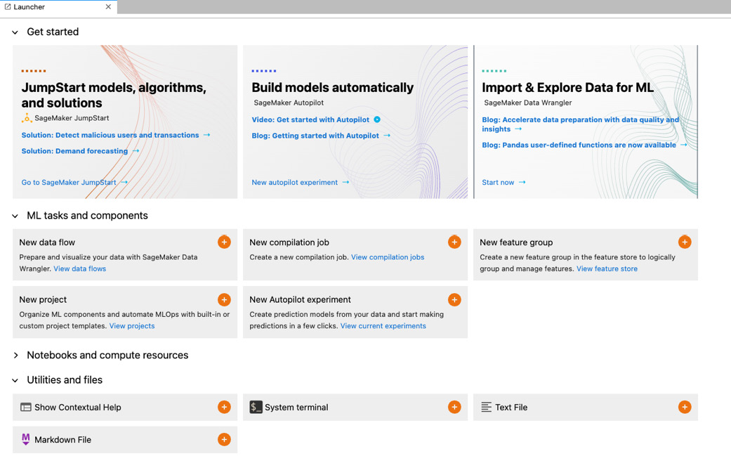
Figure 5.3 – The SageMaker Studio launcher

Note

If you have any trouble with the opening of the studio, please go back and review the prerequisite steps and then come back to this step.

3. In the Explore and prepare data for ML tile, click on Start now. This will open a page that will show a Data Wrangler is loading message. Wait for this step to complete, as it will take a few minutes. This delay is only for the first time you launch Data Wrangler.
4. Once Data Wrangler is ready, you should see a .flow file called untitled.flow. You can change the name of this file to a more relevant name such as claimsprocessing.flow in the file explorer on the left-hand panel of SageMaker studio by right-clicking on the file name.
5. In the import tab of claimsprocessing.flow, select Amazon S3. Navigate to the 2008_BSA_Inpatient_Claims_PUF.csv file. This will open up a preview panel with a sample of your claims data. Click on the Import button to import this file:

Figure 5.4 – Data preview screen in SageMaker Data Wrangler

6. On the next screen with the data flow diagram, double-click on the Data types step, which will open up the data types inferred by Data Wrangler for the columns. Except for the first column, IP_CLM_ID, which is alphanumeric, the rest of the columns are all integers. You can change them to Long. Select Long from the drop-down menu, as shown in the following screenshot, and click on Preview and then Update:

Figure 5.5 – The data type step in the Data Wrangler flow

7. Click on Add step and scroll down to the transform option, Manage columns. Make sure Drop column transform is selected in the transform drop-down list. Select IP_CLM_ID from the columns to drop drop-down list. This column is a unique identifier having no significance to ML, so we are going to drop it. Click on Preview and then Add:

Figure 5.6 – Dropping the column transform in SageMaker Data Wrangler

8. Next, we will import two more files into Data Wrangler from our dictionary. We will join these files with 2008_BSA_Inpatient_Claims_PUF.csv to bring some text attributes into our data. Click on Back to data flow and follow step 5 two more times to import the DiagnosisRelatedGroupNames.csv and InternationalClassification_OfDiseasesNames.csv files into Data Wrangler.
9. Next, repeat step 6 to change the data type of the integer column in both datasets to Long. You are now ready to join the datasets.
10. Click on the + sign next to the drop column step in the 2008_BSA_Inpatient_Claims_PUF.csv data flow. Then, click on Join:

Figure 5.7 – The Join option in SageMaker Data Wrangler

11. On the Join screen, you will see a panel where you can see the left-hand dataset already selected. Select the right-hand dataset by clicking on the Data types step next to DiagnosisRelatedGroupNames.csv. Next, click on the Preview tab:

Figure 5.8 – The Join data flow step in SageMaker Data Wrangler

12. On the Join preview screen, type in a name for your join step such as DRG-Join, and select the join type as Inner. Select the IP_CLM_BASE_DRG_CD column for both the left and right columns to join. Then, click on Preview and Add.
13. Now we will join the InternationalClassification_OfDiseasesNames.csv data. Click on the + button next to the Join step in your data flow and repeat steps 10, 11, and 12. Note that this time, the columns to join on the left and right will be IP_CLM_ICD9_PRCDR_CD.
14. As a result of the joins, there are some duplicate columns that are added to the dataset. Also, since we have long descriptive columns for DRG and procedures, we can remove the original code columns that are integers. Click on the + sign after the second join step and click on Add transform. Follow step to drop the IP_CLM_ICD9_PRCDR_CD_0, IP_CLM_ICD9_PRCDR_CD_1, IP_CLM_BASE_DRG_CD_0, and IP_CLM_BASE_DRG_CD_1 columns.
15. We are now done with feature engineering. Let us export the data to S3. Double-click on the last Drop column step and click on Export data. On the next Export data screen, select the S3 bucket where you want to export the transformed data file in CSV format. Leave all the other selections as default and click on Export data. This will export the CSV data file to S3. You can navigate to the S3 location and verify that the file has been exported by clicking on the S3 location hyperlink:

Figure 5.9 – The Export data screen in SageMaker Data Wrangler

Now that we are ready with our transformed dataset, we can begin the model training and evaluation step using SageMaker Studio notebooks.

Building, training, and evaluating the model

We will use a SageMaker Studio notebook to create a regression model on our transformed data. Then, we will evaluate this model to check whether it performs well on a test dataset. The steps for this are documented in the notebook file, which you can download from GitHub at https://github.com/PacktPublishing/Applied-Machine-Learning-for-Healthcare-and-Life-Sciences-using-AWS/blob/main/chapter-05/claims_prediction.ipynb:

1. Open the Sagemaker Studio interface.
2. Navigate to the path Applied-Machine-Learning-for-Healthcare-and-Life-Sciences-using-AWS/chapter-5/. and open the file claims_prediction.ipynb.
3. Read the notebook and complete the steps, as documented in the notebook instructions.
4. By the end of the notebook, you will have a scatter plot showing a comparison between actual and predicted values, as shown in the following screenshot:

Figure 5.10 – Scatter plot showing actual versus predicted values

This concludes our exercise. It is important to shut down the instance on which Data Wrangler and the Studio notebooks are running to avoid incurring charges. You can do so by following the instructions at the following links:

• Shutting down Data Wrangler: https://docs.aws.amazon.com/sagemaker/latest/dg/data-wrangler-shut-down.html
• Shutting down Studio: https://docs.aws.amazon.com/sagemaker/latest/dg/studio-tasks-update.html

Summary

In this chapter, we dove into the details of the healthcare insurance industry and its business model. We looked at claim processing in detail and went over different stages of how a claim gets processed and disbursed. Additionally, we looked at the various applications of ML in the claims processing pipeline and discussed approaches and techniques to operationalize large-scale claims processing in healthcare. We got an introduction to SageMaker Studio and, more specifically, SageMaker Data Wrangler and the SageMaker Studio notebooks. Lastly, we used our learnings to build an example model to predict the average healthcare claims costs for Medicare patients.

In Chapter 6, Implementing Machine Learning for Medical Devices and Radiology Images, we will dive into how medical images are generated and stored and also some common applications of ML techniques in medical images to help radiologists become more efficient. We will also get introduced to the medical device industry and how the ML models running on these devices can help with timely medical interventions.