
1
Introducing Machine Learning and the AWS Machine Learning Stack
Applying Machine Learning (ML) technology to solve tangible business problems has become increasingly popular among business and technology leaders. There are a lot of cutting-edge use cases that have utilized ML in a meaningful way and have shown considerable success. For example, computer vision models can allow you to search for what’s in an image by automatically inferring its content, and Natural Language Processing (NLP) models can understand the intent of a conversation and respond automatically while closely mimicking human interactions. As a matter of fact, you may not even know whether the “entity” on the other side of a phone call is an AI bot or a real person!
While AI technology has a lot of potential for success, there is still a limited understanding of this technology. It is usually concentrated in the hands of a few researchers and advanced partitioners who have spent decades in the field. To solve this knowledge parity, a large section of software and information technology firms such as Amazon Web Services (AWS) are committed to creating tools and services that do not require a deep understanding of the underlying ML technology and are still able to achieve positive results. While these tools democratize AI, the conceptual knowledge of AI and ML is critical for its successful application and should not be ignored.
In this chapter, we will get an understanding of ML and how it differs from traditional software. We will get an overview of a typical ML life cycle and also learn about the steps a data scientist needs to perform to deploy an ML model in production. These concepts are fairly generic and can be applied to any domain or organization where ML is utilized.
By the end of this chapter, you will get a good understanding of how AWS helps democratize ML with purpose-built services that are applicable to developers of all skill levels. We will go through the AWS ML stack and go over the different categories of services that will help you understand how the AWS AI/ML services are organized overall. We’ll cover these topics in the following sections:
- What is ML?
- Exploring the ML life cycle
- Introducing ML on AWS
What is ML?
As the name suggests, ML generally refers to the area of computer science that involves making machines learn and make decisions on their own rather than acting on a set of explicit instructions. In this case, think about the machine as the processor of a computer and the instructions as a program written in a particular programming language. The compiler or the interpreter parses the program and derives a set of instructions that the processor can then execute. In this case, the programmer is responsible for making sure the logic they have in their program is correct as the processor will just perform the task as instructed.
For example, let’s assume you want to create a marketing campaign for a new product and want to target the right population to send the email to. To identify this population, you can create a rule in SQL to filter out the right population using a query. We can create rules around age, purchase history, gender, and so on and so forth, and will just process the inputs based on these rules. This is depicted in the following diagram.
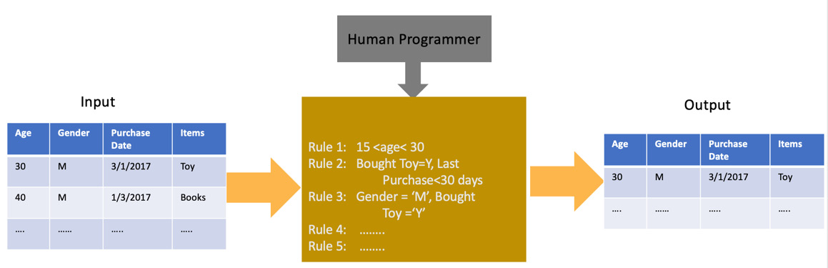
Figure 1.1 – A diagram showing the input, logic, and output of a traditional software program
In the case of ML, we allow the processor to “learn” from past data points about what is correct and incorrect. This process is called training. It then tries to apply that learning to unseen data points to make a decision. This process is known as prediction because it usually involves determining events that haven’t yet happened. We can represent the previous problem as an ML problem in the following way.

Figure 1.2 – A diagram showing how historical data is used to generate predictions using an ML model
As shown in the preceding diagram, we feed the learning algorithm with some known data points in the form of training data. The algorithm then comes up with a model that is now able to predict outputs from unseen data.
While ML models can be highly accurate, it is worth noting that the output of a model provides a probabilistic estimation of an answer instead of deterministic, like in the case of a software program. This means that ML models help us predict the probability of something happening, rather than telling us what will happen for sure. For this reason, it is important to continuously evaluate an ML model’s output and determine whether there is a need for it to be trained again.
Also, downstream consumers of an ML model (client applications) need to keep the probabilistic nature of the output in mind before making decisions based on it. For example, software to compute the sales numbers at the end of each quarter will provide a deterministic figure based on which you can calculate your profit for the quarter. However, an ML model will predict the sales number at the end of a future quarter, based on which you can predict what your profit would look like. The former can be entered in the books or ledger but the latter can be used to get an idea of the future result and take corrective actions if needed.
Now that we have a basic understanding of how to define ML as a concept, let’s look at two broad types of ML.
Supervised versus unsupervised learning
At a high level, ML models can be divided into two categories:
- Supervised learning model: A supervised ML model is created when the training data has a target variable in place. In other words, the training data contains unique combinations of input features and target variables. This is known as a labeled dataset. The supervised learning model learns the relationship between the target and the input features during the training process. Hence, it is important to have high-quality labeled datasets when training supervised learning models. Examples of supervised learning models include classification and regression models. Figure 1.3 depicts how this would work for a model that recognizes the breed of dogs.

Figure 1.3 – A diagram showing a typical supervised learning prediction workflow
- Unsupervised learning model: An unsupervised learning model does not depend on the availability of labeled datasets. In other words, unlike its supervised cousin, the unsupervised learning model does not learn the association between the target variable and the input features. Instead, it learns the patterns in the overall data to determine how similar or different each data point is from the others. This is usually done by representing all the data points in parameter space in two or three dimensions and calculating the distance between them. The closer they are to each other, the more similar they are to each other. A common example of an unsupervised learning model is k-means clustering, which divides the input data points into k number of groups or clusters.

Figure 1.4 – A diagram showing a typical unsupervised learning prediction workflow
Now that we have an understanding of the two broad types of ML models, let us review a few key terms and concepts that are commonly used in ML.
ML terminology
There are some key concepts and terminologies specific to ML and it’s important to get a good understanding of these concepts before you go deeper into the subject. These terms will be used repeatedly throughout this book:
- Algorithm: Algorithms are at the core of an ML workflow. The algorithm defines how the training data is utilized to learn from its representations, and is then used to make predictions of a target variable. An example of an algorithm is linear regression. This algorithm is used to find the best fit line that minimizes the error between the actual and the predicted values of the target. This best fit line can be represented by a linear equation such as y=ax+b. This type of algorithm can be used for problems that can be represented by linear relationships. For example, predicting the height of a person based on their age or predicting the cost of a house based on its square footage.
However, not all problems can be solved using a linear equation because the relationship between the target and the input data points might be non-linear, represented by a curve instead of a straight line. In the case of non-linear regression, the curve is represented by a nonlinear equation y=f(x,c)+b where f(x,c) can be any non-linear function. This type of algorithm can be used for problems that can be represented by non-linear relationships. For example, the prediction of the progression of a disease in a population can be driven by multiple non-linear relationships. An example of a non-linear algorithm is a decision tree. This algorithm aims to learn how to split the data into smaller subsets till the subset is as close in representation to the target variable as possible.
The choice of algorithm to solve a particular problem ultimately depends on multiple factors. It is often recommended to try multiple algorithms and find the one that works best for a particular problem. However, having an intuition of how the algorithm works allows you to narrow it down to a few.
- Training: Training is the process by which an algorithm learns. In other words, it helps converge on the best fit line or curve based on the input dataset and the target variable. As a result, it is also sometimes referred to as fitting. During the training process, the input data and the target are fed into the algorithm iteratively, in batches. The process tries to determine the coefficients of the final equation that represents the line or the curve with the minimum error when compared to the target variable. During the training process, the input dataset is divided into three different groups: train, validation, and test. The train dataset is the majority of the input data and is used to fit or train the model. The validation dataset is used to evaluate the model performance and, if necessary, tune the model input parameters (also known as hyperparameters) in an iterative way. Finally, the test dataset is the dataset on which the final evaluation of the model is done, which determines whether it can be deployed in production. The process of training and tuning the model is highly iterative. It requires multiple runs and trial and error to determine the best combination of parameters to use in the final model.
The evaluation of the ML model is done by a metric, also known as the evaluation metric, which determines how good the model is. Depending on the choice of the evaluation metric, the training process aims to minimize or maximize the value of the metric. For instance, if the evaluation metric is Mean Squared Error, the goal of the training job is to minimize it. However, if the evaluation metric is accuracy, the goal would be to maximize it. Training is a compute-intensive process and can consume considerable resources.
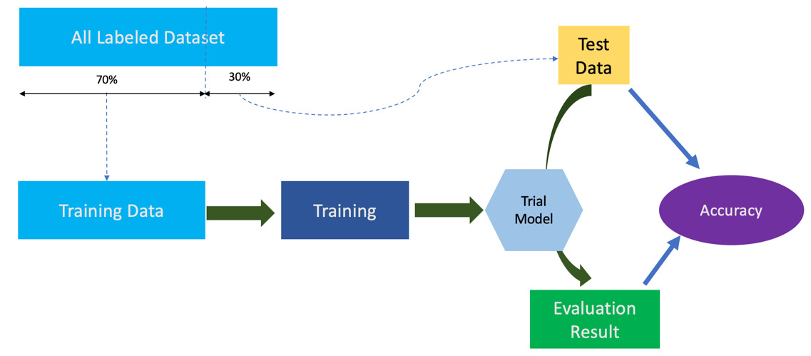
Figure 1.5 – A diagram showing the steps of a model training workflow
- Model: An ML model is an artifact that results from the training process. In essence, when you train an algorithm with data, it results in a model. A model accepts input parameters and provides the predicted value of the target variable. The input parameters should be exactly the same in structure and format as the training data input parameters. The model can be serialized into a format that can be stored as a file and then deployed into a workflow to generate predictions. The serialized model file stores the weights or coefficients that, when applied to the equation, result in the value of the predicted target. To generate predictions, the model needs to be de-serialized or reconstructed from the saved model file. The idea of saving the model to the disk by serializing it allows for model portability, a term typically used by data scientists to denote interchangeability between frameworks when it comes to data science. Common ML frameworks such as PyTorch, scikit-learn, and TensorFlow all support serializing model files into standard formats, which allows you to standardize your model registries and also use them interchangeably if needed.
- Inference: Inference is the process of generating predictions from the trained model. Hence, this step is also known as predicting. The model that has been trained on past data is now exposed to unseen data to generate the value of the target variable. As described earlier, the model resulting from the training process is already evaluated using a metric on a test dataset, which is a subset of the input data. However, this does not guarantee that the model will perform well on unseen data when deployed. As a result, prediction results are continuously monitored and compared against the ground truth (actual) values.
There are various ways in which the model results are monitored and evaluated in production. One common method utilizes humans to evaluate certain prediction results that are suspicious. This method of validation is also known as human-in-the-loop. In this method, the model results with lower confidence (usually denoted by a confidence score) are routed to a human to determine if the output is correct or not. The human can then override the model result if needed before sending it to the downstream system. This method, while extremely useful, has a drawback. Some ML models do not have the ground truth data available until the event actually happens in the future. For instance, if the model predicts a patient is going to require a kidney transplant, a human may not be able to validate that output of the model until the transplant actually happens (or not). In such cases, the human-in-the-loop method of validation does not work. To account for such limitations, the method of monitoring drift in real-world data compared to the training data is utilized to determine the effectiveness of the model predictions. If the real-world data is very different from the training data, the chances of predictions being correct are minimal and hence, it may require retraining the model.
Inferences from an ML model can be executed as an asynchronous batch process or as a synchronous real-time process. An asynchronous process is great for workloads that run in batches. For example, calculating the risk score of loan defaults across all monthly loan applications at the end of the month. This risk score is generated or updated once a month for a large batch of individuals who applied for a loan. As a result, the model does not need to serve requests 24/7 and is only used at scheduled times. Synchronous or real-time inference is when the model serves out inference as a response to each request 24/7 in real time. In this case, the model needs to be hosted on a highly available infrastructure that remains up and running at all times and also adheres to the latency requirements of the downstream application. For example, a weather forecast application that continuously updates the forecast conditions based on the predictions from a model needs to generate predictions 24/7 in real time.
Now that we have a good understanding of what ML is and the key terminologies associated with it, let’s look at the process of building the model in more detail.
Exploring the ML life cycle
The ML life cycle refers to the various stages in the conceptualization, design, development, and deployment of an ML model. These stages in the ML model development process consist of a few key steps that help data scientists come up with the best possible outcome for the problem at hand. These steps are usually repeatable and iterative and are combined into a pipeline commonly known as the ML pipeline. An ideal ML pipeline is automated and repeatable so it can be deployed and maintained as a production pipeline. Here are the common stages of an ML life cycle.

Figure 1.6 – A diagram showing the steps of an ML life cycle
Figure 1.6 shows the various steps of the ML life cycle. It starts with having a business understanding of the problem and ends with a deployed model. The iterative steps such as data preparation and model training are denoted by loops to depict that the data scientists would perform those steps repeatedly until they are satisfied with the results. Let us now look at the steps in more detail.
Problem definition
A common mistake is to think ML can solve any problem! Problem definition is key to determining whether ML can be utilized to solve it. In this step, data scientists work with business stakeholders to find out whether the problem satisfies the key tenets of a good ML problem:
- Predictive element: During the ML problem definition, data scientists try to determine whether the problem has a predictive element. It may well be the case that the output being requested can be modeled as a rule that is calculated using existing data instead of creating a model to predict it.
For example, let us take into consideration the problem of health insurance claim fraud identification. There are some tell-tale signs of a claim being fraudulent that are derivable from the existing claims database using data transformations and analytical metrics. For example, verifying whether it’s a duplicate claim, whether the claim amount is unusually high, whether the reason for the claim matches the patient demographic or history, and so on. These attributes can help determine the high-risk claim transactions, which can then be flagged. For this particular problem, there is no need for an ML model to flag such claim transactions as the rules applied to existing claim transaction data are enough to achieve what is needed. On the other hand, if the solution requires a deeper analysis of multiple sources of data and looks at patterns across a large volume of such transactions, it may not be a good candidate for rules or analytical metrics. Applying conventional analytics to large volumes of heterogeneous datasets can result in extremely complicated analytical queries that are hard to debug and maintain. Moreover, the processing of rules on these large volumes of data can be compute-intensive and may become a bottleneck for the timely identification of fraudulent claims. In such cases, applying ML can be beneficial. A model can look at features from different sources of data and learn how they are associated with the target variable (fraud versus no fraud). It can then be used to generate a risk score for each new claim.
It is important to talk to key business stakeholders to understand the different factors that go into determining whether a claim is fraudulent or not. In the process, data scientists document a list of input features that can be used in the ML model. These factors help in the overall determination of the predictive element of the problem statement.
- Availability of dataset: Once the problem is determined to be a good candidate for ML, the next important thing to check is the availability of a high-quality labeled dataset. We cannot train models without the available data. The dataset should also be clean, with no missing values, and be evenly distributed across all features and values. It should have mapping to the target variable and the target itself should be evenly distributed across the dataset. This is obviously the ideal condition and real-world scenarios may be far from ideal. However, the closer we can get to this ideal state of data, the easier it is to produce a highly accurate model from it. In some cases, data scientists may recommend to the business they collect more data containing more examples of a certain type or even more features before starting to experiment with ML methods. In other cases, labeling and annotation of the raw data by subject matter experts (SMEs) may be needed. This is a time-consuming step and may require multiple rounds of discussions with the SMEs, business stakeholders, and data scientists before arriving at an appropriate dataset to begin the ML modeling process. It is worth the time, as utilizing the right dataset ensures the success of the ML project.
- Appetite for experimentation: In a few scenarios, it is important to highlight the fact that data science is a process of experimentation and the chances of it being successful are not always high. In a software development exercise, the work involved in each phase of requirements gathering, development, testing, and deployment can be largely predictable and can be used to accurately estimate the time it will take to complete the project. In an ML project, that may be difficult to determine from the outset. Steps such as data gathering and training the tuning hyperparameters are highly iterative and it could take a long time to come up with the best model. In some cases where the problem and dataset are well known, it may be easier to estimate the time as the results have been proven. However, the time taken to solve novel problems using ML methods could be difficult to determine. It is therefore recommended that the key stakeholders are aware of this and make sure the business has an appetite for experimentation.
Data processing and feature engineering
Before data can be fed into an algorithm for training a model, it needs to be transformed, cleaned, and formatted in a way that can be understood by ML algorithms. For example, raw data may have missing values and may not be standardized across all columns. It may also need transformations to create new derived columns or drop a few columns that may not be needed for ML. Once these data processing steps are complete, the data needs to be made suitable for ML algorithms for training. As you know by now, algorithms are representative of a mathematical equation that accepts the input values of the training datasets and tries to learn its association with the target. Therefore, it cannot accept non-numeric values. In a typical training dataset, you may have numeric, categorical, or text values that have to be appropriately engineered to make them appropriate for training. Some of the common techniques of feature engineering are as follows:
- Scaling: This is a technique by which a feature that may vary a lot across the dataset can be represented at a common scale. This allows the final model to be less sensitive to the variations in the feature.
- Standardizing: This technique allows the feature distribution to have a mean value of zero and a standard deviation of one.
- Binning: This approach allows for granular numerical values to be grouped into a set, resulting in categorical variables. For example, people above 60 years of age are old, between 18 and 60 are adults, and below 18 are young.
- Label encoding: This technique is used to convert categorical features into numeric features by associating a numerical value to each unique value of the categorical variable. For example, if a feature named color consists of three unique values – Blue, Black, and Red – label encoders can associate a unique number with each of those colors, such as Blue=1, Black=2, and Red=3.
- One-hot encoding: This is another technique for encoding categorical variables. Instead of assigning a unique number to each value of a categorical feature, this technique converts each feature into a column in the dataset and assigns it a 1 or 0. Here is an example:
Price
Model
1000
iPhone
800
Samsung
900
Sony
700
Motorola
Table 1.1 – A table showing data about cell phone models and their price
Applying one-hot encoding to the preceding table will result in the following structure.
|
Price |
iPhone |
Samsung |
Sony |
Motorola |
|
1000 |
1 |
0 |
0 |
0 |
|
800 |
0 |
1 |
0 |
0 |
|
900 |
0 |
0 |
1 |
0 |
|
700 |
0 |
0 |
0 |
1 |
Table 1.2 – A table showing the results of one-hot encoding applied to the table in Figure 1.7
The resulting table is sparse in nature and consists of numeric features that can be fed into an ML algorithm for training.
The data processing and feature engineering steps you ultimately apply depend on your source data. We will look at some of these techniques applied to datasets in subsequent chapters where we will see examples of building, training, and deploying ML models with different datasets.
Model training and deployment
Once the features have been engineered and are ready, it is time to enter into the training and deployment phase. As mentioned earlier, it’s a highly repetitive phase of the ML life cycle where the training data is fed into the algorithm to come up with the best fit model. This process involves analyzing the output of the training metrics and tweaking the input features and/or the hyperparameters to achieve a better model. Tuning the hyperparameters of a model is driven by intuition and experience. Experienced data scientists select the initial parameters based on their knowledge of solving similar problems using the algorithm of choice and can come up with the best fit model faster. However, the trial-and-error process can be time-consuming for a new data scientist who is starting off with a random search of the parameters. This process of identifying the best hyperparameters of a model is known as hyperparameter tuning.
The trained model is then deployed typically as a REST API that can be invoked for generating predictions. It’s important to note that training and deployment is a continuous process in an ML life cycle. As discussed earlier, models that perform well in the training phase may degrade in performance in production over a period of time and may require retraining. It is also important to keep training the model at regular intervals with newly available real-world data to make sure it is able to predict accurately in all variations of production data. For this reason, ML engineers prefer to create a repeatable ML pipeline that continuously trains, tunes, and deploys newer versions of models as needed. This process is known as ML Operations, or simply MLOps, and the pipeline that performs these tasks is known as an MLOps pipeline.
Introducing ML on AWS
AWS puts ML in the hands of every developer, irrespective of their skill level and expertise, so that businesses can adopt the technology quickly and effectively. AWS focuses on removing the undifferentiated heavy lifting in the process of building ML models such as the management of the underlying infrastructure, the scaling of the training and inference jobs, and ensuring high availability of the models. It provides developers with a variety of compute instances and containerized environments to choose from that are purpose-built for the accelerated and distributed computing needed for high-scale ML jobs. AWS has a broad and deep set of ML capabilities for builders that can be connected together, like Lego pieces, to create intelligent applications.
AWS ML services cover the full life cycle of an ML pipeline from data annotation/labeling, data cleansing, feature engineering, model training, deployment, and monitoring. It has purpose-built services for problems in computer vision, natural language processing, forecasting, recommendation engines, and fraud detection, to name a few. It also has options for automatic model creation and no-/low-code options for creating ML models. The AWS ML services are organized into three layers also known as the AWS machine learning stack.
Introducing the AWS ML stack
The following diagram represents the version of the AWS AI/ML services stack as of April 2022.

Figure 1.7 – A diagram depicting the AWS ML stack as of April 2022
The stack can be used by expert practitioners who want to develop a project within the framework of their choice; data scientists who want to use the end-to-end capabilities of SageMaker; business analysts who can build their own model using Canvas; or application developers with no previous ML skills who can add intelligence to their applications with the help of API calls. The following are the three layers of the AWS AI/ML stack:
- AI services layer: The AI services layer of the AWS ML stack is the topmost layer of the stack. It consists of services that require minimal knowledge of ML. Sometimes, it comes with a pre-trained model that can be just invoked using APIs from the AWS SDK, the AWS CLI, or the console. In other cases, the services allow you to customize the model by providing your own labeled training dataset so the responses are more appropriate for the problem at hand. In any case, the AI services layer of the AWS AI/ML stack is focused on ease of use. The services are designed for specialized applications in industrial settings, search, business processes, and healthcare. It also comes with a core set of capabilities in the areas of speech, chatbots, vision, and text and documents.
- ML services layer: The ML services layer is the middle layer of the AWS AI/ML stack. It provides tools for data scientists to perform all the steps of the ML life cycle, such as data cleansing, feature engineering, model training, deployment, and monitoring. It is driven by the core ML platform of AWS known as Amazon SageMaker. SageMaker provides the ability to build a modular containerized environment that interfaces with the AWS compute and storage services seamlessly. It provides its own SDK that has APIs to interact with the service. It removes the complexity from each step of the ML workflow by providing simple-to-use modular capabilities with a choice of deployment architectures and patterns to suit virtually any ML application. It also contains MLOps capabilities to create a reproducible ML pipeline that is easy to maintain and scale. The ML services layer is suited for data scientists who build and train their own models and maintain large-scale models in production environments.
- ML fameworks and the infrastructure layer: The ML frameworks and infrastructure layer is the bottom layer of the AWS AI/ML stack. The services in this layer are for expert practitioners who can develop using the framework of their choice. It provides a choice for developers and scientists to run their workloads as a managed experience in Amazon SageMaker or run their workloads in a self-managed environment on AWS Deep Learning, Amazon machine images (AMIs), and AWS Deep Learning Containers. The AWS Deep Learning AMI and containers are fully configured with the latest versions of the most popular deep learning frameworks and tools – including PyTorch, MXNet, and TensorFlow. As part of this layer, AWS provides a broad and deep portfolio of compute, networking, and storage infrastructure services with a choice of processors and accelerators to meet your unique performance and budget needs for ML.
Now that we have a good understanding of ML and the AWS ML stack, it is a good time to re-read sections that may not be entirely clear. Also, the chapter introduces concepts of ML, but if you want to dive deeper into any of the concepts touched upon in this chapter, there are several trusted online resources for you to refer to. Let us now summarize the lessons from this chapter and see what’s ahead.
Summary
In this chapter, you got an overview of the basic concepts of ML. You went over the definition of ML and how it differs from typical software. You also learned about important terminologies and concepts that are heavily used in the context of ML. The chapter also covered the important steps of the ML life cycle, which can be combined together to create an end-to-end ML pipeline to deploy models in production. Lastly, you got an introduction to the AWS ML stack and how the AWS AI/ML services are organized.
In Chapter 2, Exploring Key AWS Machine Learning Services for Healthcare and Life Sciences, we will dive into the details of some of the critical AWS services that allow healthcare and life sciences customers to build, train, and deploy ML models for solving important problems in the industry. We will cover those problems in detail in the subsequent chapters of this book.