
5
Energy Function
Many of the computer vision problems at the low to intermediate levels can be considered to be labeling problems. Defined over the image plane, the labels form a function mapping that uniquely maps a set of pixels onto an attribute label. The quality of the labeling is signified with an energy function – a functional of the label function. Depending on the applications, energy functions have various different forms in their terms and relationships but have some common categories in their forms and solution methods. Finding correct representations for energy function and energy minimization methods (Heyden 2013; Szeliski et al. 2008) are key issues in vision problems.
Energy functions are found in many different domains, including optimization, Bayesian estimation, network flow (Ahuja et al. 1993; Cormen et al. 2001), and thermodynamics domains. In optimization domains, energy functions are known by various names, such as objective functions, loss functions, cost functions, and utility functions. The energy function used in thermodynamics is called (Helmholtz or Gibbs) free energy (Wikipedia 2013h) and equilibrium is the state in which the energy is at a minimum. In Bayesian estimation, the energy function is the likelihood of the ensemble probability, and the goal is often to determine the maximum a posteriori (MAP) estimate, the area where the energy is at a minimum. In a flow network, the energy is the maximum flow from the source to the sink and the purpose of graph cuts is to find the minimum cut to determine this energy. Regardless of the origin and the level of vision pathways, all the goals are to find the state in which the energy function is at a minimum. It is well known that the energy function in vision problems has the same structure, taking two common terms: data term (t-link in graph cuts terms (Boykov et al. 1998)) and smoothness term (n-link in graph cuts terms (Boykov et al. 1998)). The data term represents the likelihood, measuring the observation error between the measurement and the corresponding estimates. The smoothness term represents the prior, including the inherent statistical properties of the hidden states in nature.
Presently, the field of energy minimization is focused on the energy function model, which includes higher-order and irregular sets of partitions, and the inference methods that include linear programming relaxation (LPR), variations of message passing, and move-making algorithms in graph cuts (GC) (see (Kappes et al. 2013; Szeliski et al. 2008)).
This chapter relates how the concept of the energy equation evolves from the potential of MRF to the factor graph. In later chapters, the minimization of the energy function is studied in terms of the basic methods: relaxation (RE) machine, dynamic programming (DP) machine, belief propagation (BP) machine, and graph cuts (GC) machine.
5.1 Discrete Labeling Problem
In a labeling problem, we are given a set of objects, a set of labels for each object, a neighbor relation over the objects, and a constraint relation over labels of pairs (or n-tuples) of neighboring objects. The solution is an assignment of labels to each object in a manner that is consistent with respect to the constraint relation. The formal definition is as follows.
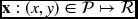
Definition5.1 (Labeling problem) Let ![]() be an instance of an image,
be an instance of an image, ![]() be a labeling, where
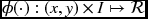
be a labeling, where ![]() is the labeling space of size L, and N( · ) be a neighborhood. A data term
is the labeling space of size L, and N( · ) be a neighborhood. A data term ![]() and a smoothness
and a smoothness ![]() for
for ![]() . The energy function is then defined by
. The energy function is then defined by
Finally, the labeling problem is defined by
Although the instance is confined to a single image, it may be generalized to a set of images of video streams. Two functions are defined in such a way that the data term depends on the label and the local instance, and the smoothness term depends on the local configuration of label distribution. The global cost is defined by the energy function, which is the sum of the data terms and the smoothness terms. All the functions are assumed to be bounded below.
This is one of the many definitions of the labeling problem, called multiclass classification. The more general definition is multi-label classification (Madjarov et al. 2012; Sorower 2010). The labeling problem is related to classification as well as the learning paradigm. According to the definition, the labeling problem becomes an optimization problem, given the energy function.
In the following, we justify the energy function by deriving it from the Markov random field (MRF) hypothesis and examine its meaning in more detail. Ensuing chapters will deal with the energy minimization directly in the paradigms: relaxation, dynamic programming, and message passing.
5.2 MRF Model
Let ![]() be a plane with N × M lattice points. On this plane is defined an image, I, and the label,
be a plane with N × M lattice points. On this plane is defined an image, I, and the label, ![]() , where
, where ![]() for a label set
for a label set ![]() . The image may be expanded to a set of images and the label to the attributes (or descriptors). The labeling problem is to find an optimal X given an image I. For stereo matching and motion estimation, the image is a pair of conjugate images and the attributes are the disparity (stereo matching) and optical flow (motion). To define the optimality, we have to define the label as random variables on the MRF plane and derive an optimal estimate of the distribution.
. The image may be expanded to a set of images and the label to the attributes (or descriptors). The labeling problem is to find an optimal X given an image I. For stereo matching and motion estimation, the image is a pair of conjugate images and the attributes are the disparity (stereo matching) and optical flow (motion). To define the optimality, we have to define the label as random variables on the MRF plane and derive an optimal estimate of the distribution.
The problem formulation can be stated with the joint distribution p(x, I) and its marginal. We assume an MRF model in which the random variables are defined by their pairwise relationships. The concept is illustrated in Figure 5.1. The image plane is defined by the column and row coordinates, ![]() . The relationship between the labels and the data is represented by a graph G = (V, E, X), where the nodes are assigned random variables (i.e. labels) and the edges the joint probability. Each node is also connected to a single node that is assigned an image pixel. In later sections, this graph will be expanded to a more general graph, specifically, factor graph and hypergraph (Wikipedia 2013d).
. The relationship between the labels and the data is represented by a graph G = (V, E, X), where the nodes are assigned random variables (i.e. labels) and the edges the joint probability. Each node is also connected to a single node that is assigned an image pixel. In later sections, this graph will be expanded to a more general graph, specifically, factor graph and hypergraph (Wikipedia 2013d).
Consequently, we now have a powerful representation scheme for the labeling in the form of a graph.
Definition 5.2 (MRF Graph Model) An MRF graph is a loopy undirected graph G = (V, E, X), where the vertex (node) V consists of ![]() and the edges E between neighbor vertices. Random variables X defined on the vertices are MRF. Dangling nodes, representing random variables I for representing image data, are attached to the pixel nodes.
and the edges E between neighbor vertices. Random variables X defined on the vertices are MRF. Dangling nodes, representing random variables I for representing image data, are attached to the pixel nodes.
MRF is compactly characterized by four properties (Wikipedia 2013g): context independence, pairwise Markov property, local Markov property, and global Markov property. Let ⊥ signify independence, | signify the conditional, and V∖{i, j} signify V − {i, j}. The context-independent property then has the following meaning:
The pairwise Markov property means that any two unadjacent variables are conditionally independent, given that all other variables are conditionally independent.
The local Markov property states that a variable is conditionally independent of all other variables given its neighbors.
Here, Ni is the set of neighbors of i, excluding itself, and c(i) = {i}∪Ni is the closed neighborhood system of i. The global Markov property means that any two subsets of variables are conditionally independent given a separating subset, XC.
Here, any path from a node in A to a node in B must pass through C. In summary, the intention of these definitions is to limit the influence of a node just to its local neighborhood so that the joint distribution can be decomposed into many fragmented factors.
The next step is to define measurable quantities on the graph so that the labeling can be stated in terms of those quantities. Fortunately, there is an indispensable theorem that states that an MRF distribution can be modeled with a factorization – in particular, Gibbs distribution (Besag 1974; Clifford 1990; Hammersley and Clifford 1971). According to the Hammersley-Clifford theorem, we have
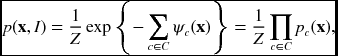
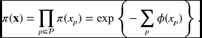
where C is a set of cliques, ψ is a clique potential, and Z is a partition function. The clique is a set of nodes such that there is an edge between every pair of nodes that are members of the set. Therefore, the joint probability is the relationship between functions defined over cliques in the graphical model. Here, the joint distribution is expressed with the measurable quantities, potential and probability.
One of the simplest cases is the regular graph with four-neighborhood, in which two types of cliques are defined: singleton and doubleton. In Figure 5.2, all the cliques for the four-neighborhood system are illustrated. For the four-neighborhood system, the distribution becomes
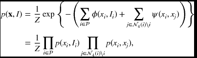
where Ni∖i = Ni − {i}. In this expression, ϕ(xi, Ii) (equivalently p(xi, Ii)) signifies the compatibility between a local observation (i.e. image) and the variable (i.e. label or attribute) and enforces a data constraint. The other term ψ(xi, xj) (equivalently p(xi, xj)) signifies a compatibility between neighboring node labels enforcing the smoothness constraint.
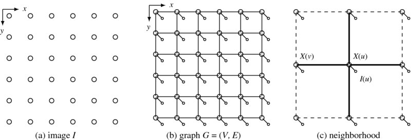
Figure 5.1 MRF model of the image
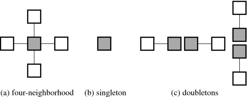
Figure 5.2 All types of cliques for a four-neighborhood system
Most of the vision problems at the low to intermediate levels lie in estimating the unknown variable X defined over the image plane, given the image I as an observation. The observation may signify an image, I, a pair of images, (Il, Ir), or a sequence of images, {(Il(t), Ir(t)|t = 0, 1, …}. The variable X signifies some attribution map defined for each pixel or parts of pixels in the image, such as image, edge, disparity, optical flow, or class label. We use x for the realization of the random variable, X.
The system is weakly described by the conditional, p(I|x), from which we can obtain the maximum likelihood (ML) estimate
The stronger description is the posterior. Bayes' rule gives
where p(x|I) is called posterior (a posteriori), p(I|x) conditional, and p(x) prior (a priori). One approach is to compute the maximum a posteriori (MAP): given I, estimate x such that
A more practical approach is to compute the marginalization:
The problem is that the complexity is exponential, which is impossible even for small problems. For instance, a problem with 100 pixels needs a search space of size 299. Fortunately, an efficient algorithm, called the belief propagation (BP) (Pearl 1982), has been introduced for such cases. Computing marginalization in an iterative manner, this method is known to be exact for Bayesian tree (i.e. BP) and approximate for loopy Bayesian networks (i.e. loopy belief propagation (LBP)).
Note that all the distributions are joint distributions. The terms usually consist of two different quantities, one that depends upon a particular problem (data term) and another that is commonplace in many vision problems (smoothness term). Exploring the one that depends on the particular problem is sometimes a major research concern. It is interesting that there exists a term that is commonplace in many problems. This term often appears as a smoothness, or regularization term, as will be seen.
5.3 Energy Function
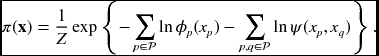
From the Hammersley–Clifford theorem, the vision problem becomes a dual problem: random variable vs. energy and statistical estimation vs. functional optimization. In this context, we study the vision problem from the energy point of view. From (5.8), we obtain the posterior:
where the positive function E(x) is called energy:
Here, the terms, called potential, are related to the density by
where the context-independent condition is used for the singleton.
In information theory, the quantities ϕ and ψ are pieces of information. In computer vision, ϕ, is called the data term (or assignment cost) and ψ the smoothness term (or prior term or separation cost). The data term is a measure of the discrepancy between observed and estimated values. The measure of smoothness is a measure of the difference between neighboring pixels.
Because of the introduction of the energy function, obtaining a MAP estimate becomes an energy minimization problem.
This approach comprises two stages: determination of the energy function and choosing the appropriate optimization technique. To fully determine the energy function, we have to define the data term and the prior term. The two terms are specific to problems and conditions. The energy minimization in the second stage belongs to unconstrained optimization and has been investigated in many areas in the computer vision field.
Among others, four approaches that have been extensively studied are variational calculus (Courant and Hilbert 1953; Horn and Shunck 1981), DP (Amini et al. 1990; Bellman 1954), BP (Pearl 1982), and graph cuts (Greig et al. 1989). There is a package in OpenCV specifically for executing and testing such algorithms (Szeliski et al. 2006): iterated conditional modes (ICM), graph cuts, max-product belief propagation, and sequential tree-reweighted message passing (TRW-S). There is also a package, called OpenGM (Bazin et al. 2013), which wraps major energy models and inference techniques into a uniform software framework for reproducible benchmarking.
The development of vision algorithms may start from either (5.8) or (5.14). The energy function approach sometimes has advantages over the probabilistic approach in that it may be considered the more general concept. Even if its origin is the factorization, the energy can be enhanced by adding more constraints than can directly be interpreted in terms of probability. The resulting energy function sometimes becomes highly nonlinear and space-variant. Because of its importance, the energy function has to be formally defined.
Definition 5.3 (Energy Function) For any given piece of data, ![]() , the energy function, E(x), is a functional defined over
, the energy function, E(x), is a functional defined over ![]() such that
such that
- The range is nonnegative real, E: x↦[0, ∞),
- x is a function satisfying
 ,
, - ϕ( · ) is a data term satisfying
 ,
, - ψ( · ) is a prior term satisfying
 .
.
In this manner, we can seek the energy function, instead of undergoing the full derivation, considering all the possible constraints that may hold in the given problem. Moreover, by doing it this way, we can generalize the energy function so that it is more general than those derived from the Markov concept.
The smoothness term originated from the clique potential, which can be interpreted as some compatibility between neighboring pixels in terms of their values. As a term in an energy function, it can be viewed as a constraint, coupled with a Lagrange multiplier, which makes the constrained problem unconstrained, so that any minimization technique for global optimization can be applied. Applying a stricter constraint to the energy function results in the search space becoming smaller and the solution getting closer to the global solution.
5.4 Energy Function Models
Thus far, we have reviewed the traditional view of the energy function in terms of MRF, which is well documented (Szeliski et al. 2008). The concept of the energy function is emerging as a mainstay called discrete energy minimization in the computer vision domain (Kappes et al. 2013).
To integrate the classical and the state-of-the-art concepts, we view the energy function in three different tasks: energy model, inference scheme, and learning. The model deals with the definition of the energy function, the inference scheme deals with the general methods for energy minimization, and the learning addresses the problems of determining system parameters.
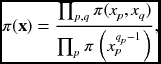
The energy model is being expanded to more general frameworks (Kappes et al. 2013): factor graph model, higher factors, larger irregular graphs, and a group of pixels instead of a single pixel. As such, the MRF in Definition 5.2 must be expanded to the factor graph (Kappes et al. 2013; Koller and Friedman 2009).
Definition 5.4 (MRF Factor Graph) Define an MRF factor graph, G = (U, V, X, Θ), as a vertex weighted directed bipartite graph, where U is the factor nodes, V is the variable nodes, X = {xv|v ∈ V} is the MRF variables, and Θ = {θu(xu)|xu = {xv|v ∈ Nu}, u ∈ U} is the factors.
Note that Nu is a set of variable nodes, which are connected to the factor node u.
According to the above definition, terms in the traditional MRF energy model are replaced with the functions of factors. The factor F defines every relationship in the general graph, including node-to-node (binary potential, smoothness term, or compatibility term) and node-to-data (unary potential, data term, or data fidelity), by its associated function sets. Thus, the representation becomes more general and explicit than the original MRF model, which is defined by an undirected graph.
There are several aspects of model G that explicitly characterize the target vision problem (Kappes et al. 2013) (e.g. stereo matching, motion estimation, and color segmentation) in terms of complexity and graph topology (Kappes et al. 2013). The number of possible labels is important since it is directly related to the feasibility of the algorithm. A larger dimension label space results in an increment of complexity in computation and memory. The properties of the graph, such as regularity and order, are also important cues for categorizing the model. The graph order is decided by the maximal degree among all factors in the graph. It directly indicates the complexity of interconnections between nodes in the graph. The regular graph assumption enables us to implement inference algorithms using massive computation methods that are preferred in VLSI, or other hardware-based algorithms. As the final aspect, we can consider the properties of the associated function (potential/energy function). This functional property affects the accuracy of the model and the feasibility of the corresponding inference algorithms. Energy functions based on high-order polynomials can describe a more complex vision environment, while optimizations on these functions are infeasible in many cases.
The general energy function on the factor graph model above is defined as
where Nf denotes neighborhood factors such as observation or other neighboring nodes in the MRF representation. Since this energy model can represent far more complex vision models (i.e. higher-order graphs or energy functions, and irregular graph representations) owing to its generality, we would like to confine our discussion to three major early vision applications: stereo matching, motion estimation, and image segmentation.
Because early vision labels depend on raw image observations rather than high-level information, the order of their factor graph model is at most two. Hence, we can consider only pairwise relationship to model the target problem. This fact simplifies the corresponding energy model, which only consists of data and smoothness terms. Moreover, most of the early vision algorithms are pixel-based, so we can assume that, except for the boundary points, the graphs are regular. Neighborhood systems for early vision applications are usually defined by four-neighbors because of the trade-off between performance and complexity. Nevertheless, there might be a more general representation beyond the factor graph, which includes complicated factors such as the tripartite graph (Memisevic 2013). The remaining issues on different applications are the label dimensions, additional parameters, and the functional properties of energy terms.
The detailed form of the energy model depends on the problem domains. In the following sections, we review only three domains: stereo matching, motion estimation, and segmentation. In the stereo matching domain, the goal is to recover hidden correspondences between pixels from different views. Therefore, the disparity value that defines the correspondences becomes the target label to infer. For basic observation, although a variety of cues are available, such as image color/intensity, gradient, or color segments, we consider image color/intensity as our primary consideration for simplicity.
5.5 Free Energy
All Bayesian inferences (Roweis and Ghahramani 1999) can be cast in terms of free energy minimization. When free energy is minimized with respect to internal states, the Kullback–Leibler divergence between the variational and posterior density over hidden states is minimized. This corresponds to approximate Bayesian inference when the form of the variational density is fixed, and exact Bayesian inference otherwise. Free energy minimization therefore provides a generic description of Bayesian inference and filtering (e.g. Kalman filtering).
The distance between the two distributions can be defined by the statistical divergence (Pardo 2005; Wikipedia 2013b). Among the many, the Kullback–Leibler (KL) divergence is frequently used for free energy computation. The KL divergence is a premetric measure, and its quantities can be interpreted via information theory. Thermodynamics analogy is possible but very limited because there are physical factors missing (specifically, pressure, volume, and temperature) from the statistical model. For a true pmf, p(x), assume an approximate π(x). The KL divergence is
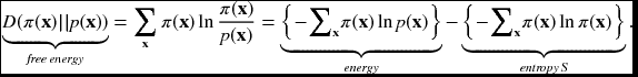
The use of the true and approximate pmfs is opposed to the original order. The divergence consists of two terms – cross-entropy (or energy) and entropy. A specific example is that when the distribution is Gaussian, the entropy is unity. The entropy is the lower bound of the energy and the energy is the upper bound of the entropy. One can optimize either of the two terms, which are bounded below or above. The gap between the energy and entropy is the free energy that must be minimized for an optimal distribution, which is supposed to be in a state of equilibrium.
The general model of the system is Boltzmann's law ![]() , where k is the Boltzmann constant and T is the temperature. We set kT = 1 if the temperature is constant or annealing is not considered.
, where k is the Boltzmann constant and T is the temperature. We set kT = 1 if the temperature is constant or annealing is not considered.
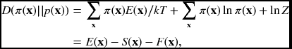
where F(x) = −ln Z is the analogy of the Helmholtz free energy, which is defined as − kTln Z. Further, S(x) = −∑xπ(x)ln π(x) is the entropy and E(x) = ∑xπ(x)ln E(x) is the internal energy. The approximate distribution is achieved by minimizing E − S, which is bounded below by the Helmholtz free energy.
Algorithms largely depend upon the models of the approximate distribution, π(x). The mean field approximation models the joint pmf using the products of singletons:
The pairwise MRF is
The Bethe free energy is
where qp is the number of nodes neighboring node p (Pearl 1988). It is known that there is a close connection between the BP algorithm and the Bethe approximation: BP can only converge to a fixed point that is also a stationary point of the Bethe approximation to the free energy (Yedidia et al. 2005).
The free energy is related to the function of the biological system. Biological systems maintain their order by restricting themselves to a limited number of states and minimize a free energy function of their internal states, which entail beliefs about hidden states in their environment. The minimization of variational free energy is formally related to variational Bayesian methods and was originally introduced by Karl Friston, as active inference (Friston et al. 2006; Wikipedia 2013c).
5.6 Inference Schemes
Energy functions can model various quantities and interactions in computer vision applications. The only remaining task is to solve for a target quantity that minimizes its corresponding energy function, called the inference. Unfortunately, searching for the global optimal solutions for a discrete energy function is intrinsically an NP-hard problem owing to its combinatorial nature. Hence, there are innumerable works about the inference method from the perspective of discrete optimization. Traditional inference methods on discrete energy functions are based on various ideas from the area of optimization, such as variational calculus (VC), iterated conditional modes (ICM) (Besag 1986), simulated annealing (SA) (Kirkpatrick et al. 1983), and dynamic programming (DP) (Bertsekas 2007), to name a few. Further, there are numerous inference schemes that were successful in other areas, such as genetic programming (GP) (Banzhaf et al. 2001) and reinforcement learning (Sutton and Barto 1998).
Presently, the representative inference methods can be categorized as follows (Kappes et al. 2013): polyhedral and combinational methods, message passing methods, max-flow and move-making methods, and deep learning. The polyhedral and combinatorial methods are based on linear programming (LP) relaxation. In these methods, the original discrete optimization problem is represented by integer linear problems (ILP) that confine target solutions to finite-range integers in local polytope. Since this ILP is NP-hard, it is relaxed by several subproblems that can be solved by LP in polynomial time. There are two major methods in LP relaxation – the Cutting Plane (CP) method (Sontag et al. 2008) and the branch-and-bound (BB) method (Sun et al. 2012). Under tight bounding conditions, the solution from LP relaxation methods is guaranteed to be the global optimal solution. The message passing methods originated from the Belief Propagation (BP) (Pearl 1988) for acyclic graphs. The most popular message passing method in vision applications is loopy belief propagation (LBP) (Szeliski et al. 2008), which is an extension of the original BP to graphs with cycles. Although LBP has no confidence on optimality of the solution, it works well practically in many vision applications. At present, polyhedral methods are often reformulated by message passing algorithms, for example, the tree-reweighted algorithm (TRWS) (Kolmogorov 2006), its nonsequential version (TRBP) (Wainwright et al. 2005), and max-product linear programming (MPLP) algorithm (Globerson and Jaakkola 2007). In contrast to the case with LBP, the convergence of solutions is guaranteed with tight bounding conditions. Message passing algorithms are easily implemented and converted into parallel architecture. The max-flow and move-making methods are based on the graph cuts (GC) (Boykov and Kolmogorov 2004). This class includes QPBO (Rother et al. 2007), α- expansion (α − β swap) (Boykov et al. 2001), FastPD (Komodakis and Tziritas 2007), and α-FUSION (Fix et al. 2011). Deep learning is a newly emerging method (Bengio et al. 2013; Hinton 2007) among the current inference techniques.
A typical example of LP relaxation is as follows (Bazin et al. 2013). Let us consider the image planes, ![]() , the images (Il, Ir), and the feature descriptors, (Fl, Fr), where
, the images (Il, Ir), and the feature descriptors, (Fl, Fr), where ![]() . For the two images, an assignment matrix,
. For the two images, an assignment matrix, ![]() , where z is one if there is a match and zero otherwise, and the distance,
, where z is one if there is a match and zero otherwise, and the distance, ![]() , are defined. Additionally, let Aij be the data associated with the input data pairs and θ be the model parameters between the data pairs, such as the fundamental matrix. The mixed integer optimization problem (MIOP) is defined as follows:
, are defined. Additionally, let Aij be the data associated with the input data pairs and θ be the model parameters between the data pairs, such as the fundamental matrix. The mixed integer optimization problem (MIOP) is defined as follows:
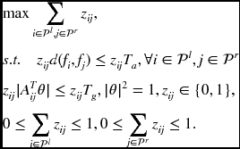
Here, Ta and Tg are the parameters for the appearance and geometric terms.
This MIOP cannot be solved directly because of the nonlinear terms. Various methods can be used to convert the MIOP to LP relaxation. First, the bilinear terms, Ta and Tg, can be made linear (Chandraker and Kriegman 2008; Kahl et al. 2008; Olsson et al. 2009). Let c = ab, with ![]() and
and ![]() , where
, where ![]() and
and ![]() . The bilinear term can then be relaxed by the convex and concave envelopes:
. The bilinear term can then be relaxed by the convex and concave envelopes:
The second technique is for the unknown bounds for θ. The branch-and-bound (BB) (Breuel 2003; Land and Doig 1960) is a general global optimization method that iteratively divides the search space into smaller ones and removes the spaces that contain poor solutions. If the lower bound for some space is greater than the upper bound for some other space, then the space may be safely discarded from the search. Using these methods, the MIOP can be converted to LP relaxation.
Another useful example of LP relaxation is MPLP (Globerson and Jaakkola 2007), which converts MAP problems in 2D MRF to MAP-LP relaxation problems. The original MAP problem is defined by energy functions comprising pairwise potentials,
LP relaxation on the energy model begins from defining marginal distribution over variables in edge set E:
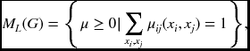
where ML is the local marginal polytope satisfying ![]() .
.
The resulting LP relaxation is given by
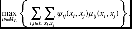
The solution to this LP relaxation problem is the upper bound of the MAP solution satisfying
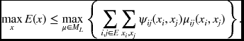
This is called edge consistent LP relaxation because marginals are constrained to be pairwise consistent. Given the LP relaxation of a MAP problem, a variety of ILP solving techniques can be applied, including CP or BB, to the primal or dual problem domain.
Solutions in the primal domain can be directly computed from standard LP algorithms for small problems. Unfortunately, most vision problems have a large solution scale, which makes primal solution practically infeasible. To tackle large problems, the dual problem of the original LP relaxation problem is widely used (Globerson and Jaakkola 2007; Kappes et al. 2012; Kolmogorov 2006; Komodakis and Paragios 2008; Sontag et al. 2008; Werner 2007) to provide the lower bound of the primal solution.
Neural networks are emerging with a new tool called deep learning, by which the layers are trained in two steps: pre-training and global training. Neural network studies are in many different directions (Bengio et al. 2013), such as probabilistic inference (i.e. restricted Boltzmann machine (RBM)), autoencoder framework, and manifold learning.
We will address the message-passing and the move-making methods in later chapters. In particular, we will focus on design for the relaxation, DP, and BP, which have the basic computational structures such as pipelining, iteration, and neighborhood computation.
5.7 Learning Methods
Before going further, let us consider the learning issues on the MRF model. Generally, an MRF system consists of a set of system parameters θ that defines its behavior under various conditions and environments. For example, we can easily consider the parametric model for observation noise. Under the Gaussian assumption, these parameters are the mean and variance of the noise. Further, for stereo applications, regularization weight is adjusted with respect to input image data to provide a more accurate matching result. The MRF model is, therefore, completely characterized by the distribution p(x|I, θ), where θ is another hidden variable. Obtaining optimal system parameters for a given environment is a very important task in the labeling problem, and can be accomplished by a number of optimization approaches.
However, true observations on the label, x, are not given in most vision problems. Therefore, supervised learning methods, which are relatively simpler than unsupervised methods, cannot be applied to recover an optimal parameter solution for a given system. To find the optimal system parameter for marginal likelihood p(x, I|θ) under an unsupervised configuration, iterative labeling-estimation (Besag 1986; Bouman and Shapiro 1994; Kelly et al. 1988; Zhang 1992) alternate the labeling and estimation process while the other side is fixed. The expectation maximization (EM) algorithm (Dempster et al. 1977; McLachlan and Krishnan 1997) provides theoretical fundamentals and formalism for these iterative algorithms.
The purpose of the EM algorithm is to simultaneously search for the latent parameter θ and the label x that maximize the marginal distribution p(x, I|θ). The optimization strategy of the EM algorithm is to divide the original optimization problem into two steps: E-step (expectation) and M-step (maximization). In the E-step, the inference on the label is tried while fixing the parameters:
During this process, the conditional distribution given the image observation and fixed parameter estimates is maximized by latent label data x, to provide expectation of target marginal likelihood p(x, I|θ).
In the M-step, learning is achieved by maximizing previously computed expectations along the parameter space.
The E-step and M-step are iterated until the resulting parameters are converged. Final parameters are maximum likelihood solutions for the marginal distribution.
In addition to the EM framework, there are a number of works that cope with the MRF parameter estimation problem, such as iterative conditional estimation (ICE) (Giordana and Pieczynski 1997), least square estimation (Borges 1999; Derin and Elliott 1987), Markov chain Monte Carlo (MCMC) (Descombes et al. 1999), simulated annealing (Lakshmanan and Derin 1989), and other artificial intelligence algorithms (Yu 2012). In stereo contexts, empirical decision on parameters were popular since including the parameter learning process makes a problem more complex. Recently, a number of works related to learning MRF for stereo matching have been presented (Cheng and Caelli 2007; Huq et al. 2008; Trinh and McAllester 2009; Zhang and Seitz 2007). In NN frameworks, the learning of deep architectures is actively underway for both representation and parameters (Bengio et al. 2013).
5.8 Structure of the Energy Function
Although the energy function is rooted in MRF factorization, algorithms dealing with advanced problems often start directly from energy functions that are far more sophisticated than can be interpreted as graphical models. The original labeling problem, which was interpreted as an estimation problem in probability, becomes a matching problem, which is interpreted as an optimization problem in the energy function.
Basic categorization data and smoothness terms are too simple for many problems. In general, the two terms can be divided into more detailed terms. Let us now return to the posterior:
The prior and the conditional terms are the origins of the smoothness and data terms. In many cases, the variables can be factorized and partitioned into regular or irregular sizes:
which results in the energy equation:
The first term, collectively called the data term (or appearance model), actually consists of many heterogeneous terms. Analogously, the second term, collectively called the smoothness term (or geometrical constraint), actually denotes many heterogeneous terms representing geometric properties between partitions.
It is possible that in the future the structure of the energy function will become more sophisticated, revealing properties that are common and general but not yet discovered. For example, in (Choi et al. 2013), the data term is divided into the target observation and the feature observations terms. The smoothness term is divided into the camera, target, and geometric feature terms. Another example is that presented by Torresani (Torresani et al. 2013), in which the energy function, consisting of appearance, occlusion, geometry, and coherence terms, is interpreted as a graph-matching problem:
where the weights are included inside the terms. The appearance and the geometry terms are the generalizations of the data and the smoothness terms. The occlusion terms are introduced for indeterminate positions and the coherence terms are introduced for the collective values of the neighborhoods.
Although roughly stated with data and smoothness terms, the detailed form of (5.33) depends upon the problems. In image restoration, it may depend on only one image but in motion or stereo vision it may depend on more than one image. The data term may have the form
where ![]() is an estimation of the input data Ii by the variable xi). The distance function is a measure between the true and estimated data.
is an estimation of the input data Ii by the variable xi). The distance function is a measure between the true and estimated data.
Unlike the data term, the smoothness term is rather general. Nevertheless, there are many variations on its forms and usage. Returning to the derivation, the smoothness term originated from the joint distribution p(xi, xj), meaning some homogeneity in doubletons:
In images, the prior of doubletons is related to the smoothness of the surface, which is often modeled as a smoothness measure using the differential.
The smoothness measure often uses the Lp − norm, especially with p = 1 or p = 2. Among the measures, L1 is the baseline measure in compressed sensing (Candes and Wakin 2008; Candès et al. 2006; Donoho 2006). In other applications, L2 is often used because of its differentiability. Various models exist (Xu et al. 2012): linear model or quadratic model, truncated quadratic, Potts model, generalized Potts model, Charbonnier (Bruhn et al. 2005) and Lorentzian (Black and Anandan 1996).
Let x = xp − xq. Then, the possible measures are as follows:
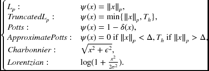
Here, δ( · ) is a Kronecker delta and ε, σ, γ, Th > 0 are parameters. The smoothness functions are illustrated in Figure 5.3.
The smoothness term can be made anisotropic so that different smoothness may be applied to different directions in accordance with the local conditions. The quadratic measure can be written as
If ψ( · ) is in a certain form, ∇E( · ) becomes an anisotropic diffusion function:
The anisotropic diffusion term performs well in preserving boundaries while smoothing the surfaces. As was proved in (Wikipedia 2013a), it can be shown that the energy equation and the diffusion are related by
As we will see, because of this property, the Euler–Lagrange equation of the energy equation contains the anisotropic diffusion term. In other optimization methods that directly minimize the energy function, the prior must be satisfied with the condition in Equation (5.40).
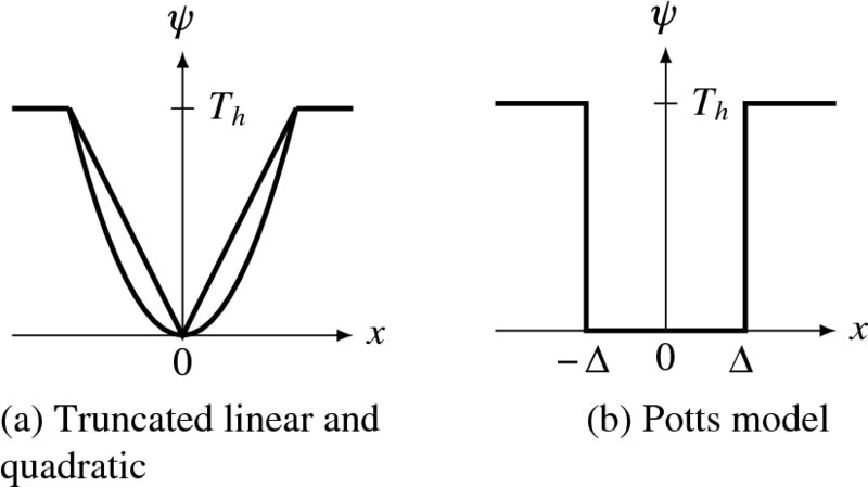
Figure 5.3 Graphs for the prior functions (Th, Δ: threshold)
The smoothness term is related to the distance measures, which are numerous in definition, including methods such as earth mover's distance (EMD) (Rubner et al. 1997 2000), Bhattacharyya coefficients (Bhattacharyya 1946; Comaniciu et al. 2003), and β-divergence (Cichocki et al. 2006). However, the practical design prefers less computation and simpler circuits, as typified by the Potts model and the linear truncated function (see the problems at the end of this chapter).
5.9 Basic Energy Functions
Let us begin with the energy function in Definition 5.1. The data term is problem dependent but the smoothness term is more general in many problems. This term is naturally involved with differentials. In this model, the neighborhood operation is replaced with differentials. If we consider up to the second-order derivative, the energy function becomes
where λ and μ are the Lagrange multipliers. The smoothness term contains a gradient and a Laplacian, which measure the roughness up to the second order derivative. A more advanced model may be
where η(x, y) is a switch function indicating possible discontinuities, such as occlusion or object boundary. Inclusion of such a nonlinear factor may require very different methods to find a solution.
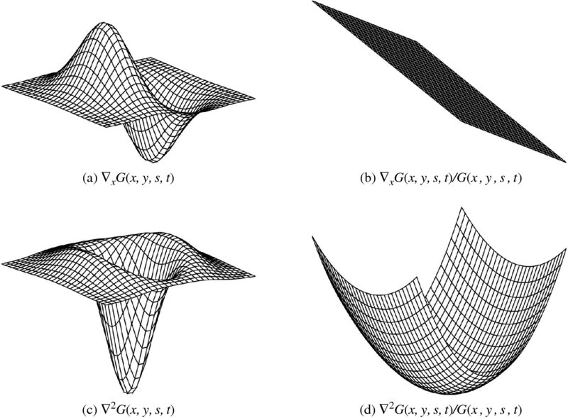
Figure 5.4 Shapes of Gaussian derivatives (here, s = 0.15 and t = 0.2)
The differentiation must be preceded by a smoothing operation, such as Gaussian filter. The combined smoothing and differentiation can be considered as filtering with Gaussian differentials. This concept can give us the meaning of the properties of the smoothness term. It is easy to get
The shape of the responses is illustrated in Figure 5.4. The Gaussian is considered anisotropic, s ≠ t, to observe more intuition of the smoothing effects. The first row shows the first derivative Gx and Gx/G. Gx detects variations in the x-axis and Gy detects variations in the y-axis. The second row shows the ∇G and ∇2G/G. This operator detects the zero crossing (ZC), signifying possible edges. It is well-known that the Laplacian is related with retinal response on edges and approximated with DOG (Marr and Hildreth 1980).
The energy function can specify various vision modules. However, a problem exists because it has no unique representation for a given module, since different applications may emphasize different aspects of the data and smoothness terms. However, there exist several fundamental forms, in which the terms appear to be essential, even if some delicate features are missing. Among the vision modules, some representative problems are image restoration, stereo vision, and motion estimation.
The goal of image restoration is to recover an original image from a corrupted one by removing as much of the effects of noise as possible. Here is a challenge: for a given I(x, y), restore the estimated image f(x, y). The energy function is defined as
Here, λ is introduced as a Lagrange multiplier that adjusts the weight of the two terms.
Stereo vision is one of the major applications of the MRF model. To facilitate a concise description, we assume that the stereo vision system has perfectly calibrated binocular cameras, and that the disparity map is left-referenced. The goal is to estimate a dense disparity map D(x, y) between two input images IL(x, y), Ir(x, y), which can be easily represented as the 2D labeling problem in the image plane. Fundamentally, the entire energy function to be minimized is defined as
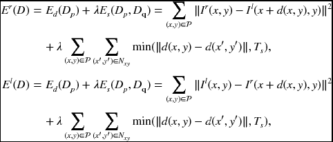
where Ts is the threshold for truncation. The singleton Ed(Dp) usually includes photo-consistency constraints between the left and right images. The doubleton Es(Dp, Dq) is the smoothness term (see the problems at the end of this chapter).
The goal of motion estimation is to estimate the motion vector between two consecutive image frames in a video sequence. Hence, the input is two images, It(x, y) and It + 1(x, y), and the target attribute is a 2D array of motion vectors ![]() . Because the two corresponding pixels in adjacent frames can be warped forward and backward with respect to the motion vector value of a particular position in reference view, the motion estimation problem can intuitively be considered an extension of the stereo vision problem. Generally, an energy function for motion estimation is defined as
. Because the two corresponding pixels in adjacent frames can be warped forward and backward with respect to the motion vector value of a particular position in reference view, the motion estimation problem can intuitively be considered an extension of the stereo vision problem. Generally, an energy function for motion estimation is defined as
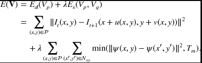
The format is very similar to that of the stereo case; in fact, disparity is changed into a motion vector quantity. Truncated quadratic form is preferred in motion estimation problems.
In later chapters, we will design the circuits for stereo matching, modifying the energy function to more appropriate forms for practical implementation.
Problems
- 5.1 [Labeling] For an image with M × N 8-bit pixels, how many labels may exist? For M = N = 100, what is the total number of labels?
- 5.2 [Labeling] For the previous search space, a computer algorithm is going to search for an optimal solution. If 1ns is needed to test a label, how long will it take to inspect all the space?
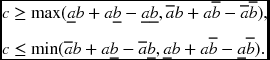
- 5.3 [Inference] Check the relationship in Equation (5.23).
- 5.4 [Inference] In Equation (5.23), the ordinary bound is
 . The new lower and upper bounds must be better than the ordinary bound. How much better are the new bounds than the ordinary ones?
 - 5.5 [Structure] Some algorithms such as Bayesian estimates, simulated annealing, and graph cuts, are driven by various probability distribution functions, such as uniform, Gaussian, Laplacian, and Gibbs distributions. There are numerous pseudorandom number generators (PRNG) (refer to the lists in (Wikipedia 2013f). The uniform distribution is a versatile distribution that can be used to derive other distributions. One of the simplest uniform distributions is the linear feedback shift register (LFSR) (Wikipedia 2013e), a shift register whose input bit is a linear function of its previous state. There are versions for Fibonacci, Galois, and maximal-length. Design a 20-bit maximal-length LFSR using the table in (Koopman 2013).
- 5.6 [Structure] Design a PRGN that generates ones with a probability of 1/2n, where n is a positive integer.
- 5.7 [Structure] In some applications, such as simulated annealing and graph cuts, we randomly select samples in a window, say a 10 × 10 window. Design such a circuit with the LFSR.
- 5.8 [Structure] Among the loss (error) functions, design a truncated linear function.
- 5.9 [Structure] Among the loss (error) functions, design a Potts model in Verilog HDL.
- 5.10 [Basic Energy] Equation (5.45) is defined for the right image plane as a reference. Write the same form for the left image plane.
References
- Ahuja RK, Magnanti TL, and Orlin JB 1993 Network Flows: Theory, Algorithms, and Applications. Prentice Hall.
- Amini AA, Weymouth TE, and Jain RC 1990 Using dynamic programming for solving variational problems in vision. IEEE Trans. Pattern Anal. Mach. Intell. 12(9), 855–867.
- Banzhaf W, Nordin P, Keller RE, and Francone FD 2001 Genetic Programming – An Introduction; On the Automatic Evolution of Computer Programs and its Applications third edn. Morgan Kaufmann, dpunkt.verlag.
- Bazin J, Li H, Kweon IS, Demonceaux C, Vasseur P, and Ikeuchi K 2013 A branch-and-bound approach to correspondence and grouping problems. IEEE Trans. Pattern Anal. Mach. Intell. 35(7), 1565–1576.
- Bellman R 1954 The theory of dynamic programming. Bulletin of the American Mathematical Society 60, 503–516.
- Bengio Y, Courville AC, and Vincent P 2013 Representation learning: a review and new perspectives. IEEE Trans. Pattern Anal. Mach. Intell. 35(8), 1798–1828.
- Bertsekas DP 2007 Dynamic Programming and Optimal Control vol. 1,2. Athena Scientific.
- Besag J 1974 Spatial interaction and the statistical analysis of lattice systems. Journal of the Royal Statistical Society, Series B 36, 192–236.
- Besag J 1986 On the statistical analysis of dirty pictures. Journal Royal Statistical Society B-48(3), 259–302.
- Bhattacharyya A 1946 On a measure of divergence between two multinomial populations. The Indian Journal of Statistics (1933–1960) 7(4), 401–406.
- Black MJ and Anandan P 1996 The robust estimation of multiple motions: Parametric and piecewise-smooth flow fields. Computer Vision and Image Understanding 63(1), 75–104.
- Borges CF 1999 On the estimation of Markov random field parameters. IEEE Trans. Pattern Anal. Mach. Intell. 21(3), 216–224.
- Bouman C and Shapiro M 1994 A multiscale random field model for Bayesian segmentation. IEEE Trans. Pattern Anal. Mach. Intell. 3(2), 162–177.
- Boykov Y and Kolmogorov V 2004 An experimental comparison of min-cut/max-flow algorithms for energy minimization in vision. IEEE Trans. Pattern Anal. Mach. Intell. 26(9), 1124–1137.
- Boykov Y, Veksler O, and Zabih R 1998 Markov random fields with efficient approximations International Conference on Computer Vision and Pattern Recognition (CVPR).
- Boykov Y, Veksler O, and Zabih R 2001 Fast approximate energy minimization via graph cuts. IEEE Trans. Pattern Anal. Mach. Intell. 23(11), 1222–1239.
- Breuel TM 2003 Implementation techniques for geometric Branch-and-Bound matching methods. Computer Vision and Image Understanding 90(3), 258–294.
- Bruhn A, Weickert J, and Schnorr C 2005 Lucas/Kanade meets Horn/Schunck: Combining local and global optic flow methods. International Journal of Computer Vision 61(3), 211–231.
- Candes E and Wakin M 2008 An introduction to compressive sampling. IEEE Signal Processing Magazine 25(2), 21–30.
- Candès EJ, Romberg JK, and Tao T 2006 Stable signal recovery from incomplete and inaccurate measurements. Comm. Pure Appl. Math. 59(8), 1207–1223.
- Chandraker M and Kriegman DJ 2008 Globally optimal bilinear programming for computer vision applications CVPR, pp. 1–8.
- Cheng L and Caelli T 2007 Bayesian stereo matching. Computer Vision and Image Understanding 106(1), 85–96.
- Choi W, Pantofaru C, and Savarese S 2013 A general framework for tracking multiple people from a moving camera. IEEE Trans. Pattern Anal. Mach. Intell. 35(7), 1577–1591.
- Cichocki A, Zdunek R, and Amari Si 2006 Csiszar divergences for non-negative matrix factorization: Family of new algorithms Independent Component Analysis and Blind Signal Separation Springer pp. 32–39.
- Clifford P 1990 Markov random fields in statistics In Disorder in Physical Systems. A Volume in Honour of John M. Hammersley (ed. Grimmett GR and Welsh DJA), pp. 19–32. Clarendon Press, Oxford.
- Comaniciu D, Ramesh V, and Meer P 2003 Kernel-based object tracking. IEEE Trans. Pattern Anal. Mach. Intell. 25(5), 564–577.
- Cormen T, Rivest CLR, and Stein C 2001 Introduction to Algorithms second edn. The MIT Press.
- Courant R and Hilbert D 1953 Methods of Mathematical Physics, vol. 1. Interscience Press.
- Dempster A, Laird N, and Rubin D 1977 Maximum likelihood from incomplete data via the em algorithm. Journal of the Royal Statistical Society, Series B 39, 1–38.
- Derin H and Elliott H 1987 Modeling and segmentation of noisy and textured images using Gibbs random fields. IEEE Trans. Pattern Anal. Mach. Intell. 9(1), 39–55.
- Descombes X, Morris RD, Zerubia J, and Berthod M 1999 Estimation of Markov random field prior parameters using Markov chain Monte Carlo maximum likelihood. IEEE Trans. Image Processing 8(7), 954–963.
- Donoho D 2006 Compressed sensing. IEEE Trans. Information Theory 52(4), 1289–1306.
- Fix A, Gruber A, Boros E, and Zabih R 2011 A graph cut algorithm for higher-order Markov random fields In ICCV (ed. Metaxas DN, Quan L, Sanfeliu A, and Gool LJV), pp. 1020–1027. IEEE.
- Friston K, Kilner J, and Harrison L 2006 A free energy principle for the brain. J Physiol Paris. 100(1-3), 70–87.
- Giordana N and Pieczynski W 1997 Estimation of generalized multisensor hidden Markov Chain and unsupervised image segmentation. IEEE Trans. Pattern Anal. Mach. Intell. 19(5), 465–475.
- Globerson A and Jaakkola T 2007 Fixing max-product: Convergent message passing algorithms for MAP LP-relaxations In NIPS (ed. Platt JC, Koller D, Singer Y, and Roweis ST). Curran Associates, Inc.
- Greig D, Porteous B, and Seheult A 1989 Exact maximum a posteriori estimation for binary images. Journal of the Royal Statistical Society Series B 51, 271–279.
- Hammersley J and Clifford P 1971 Markov fields on finite graphs and lattices Unpublished note.
- Heyden A 2013 Energy minimization methods in computer vision and pattern recognition 9th International Conference, EMMCVPR 2013 CVPR.
- Hinton GE 2007 Learning multiple layers of representation. Trends in Cognitive Science 11(10), 428–434.
- Horn B and Shunck B 1981 Determining optical flow. Artificial Intelligence 17(1-3), 185–203.
- Huq S, Koschan A, Abidi B, and Abidi M 2008 Efficient BP stereo with automatic parameter estimation 15th IEEE International Conference on Image Processing, pp. 301–304.
- Kahl F, Agarwal S, Chandraker MK, Kriegman DJ, and Belongie S 2008 Practical global optimization for multiview geometry. International Journal of Computer Vision 79(3), xx–yy.
- Kappes JH, Andres B, Hamprecht FA, Schnorr C, Nowozin S, Batra D, Kim S, Kausler BX, Lellmann J, Komodakis N, and Rother C 2013 A comparative study of modern inference techniques for discrete energy minimization problems EMMCVPR 2013.
- Kappes JH, Savchynskyy B, and Schnorr C 2012 A bundle approach to efficient MAP-inference by Lagrangian relaxation CVPR, pp. 1688–1695.
- Kelly PA, Derin H, and Hartt KD 1988 Adaptive segmentation of speckled images using a hierarchical random field model. IEEE Trans. Acoustic, Speech and Signal Processing 36, 1628–1641.
- Kirkpatrick S, Jr. DG, and Vecchi MP 1983 Optimization by simmulated annealing. Science 220(4598), 671–680.
- Koller D and Friedman N 2009 Probabilistic Graphical Models: Principles and Techniques. MIT Press.
- Kolmogorov V 2006 Convergent Tree-reweighted message passing for energy minimization. IEEE Trans. Pattern Anal. Mach. Intell. 28(10), 1568–1583.
- Komodakis N and Paragios N 2008 Beyond loose lp- relaxations: Optimizing MRFs by repairing cycles ECCV.
- Komodakis N and Tziritas G 2007 Approximate labeling via graph cuts based on linear programming. IEEE Trans. Pattern Anal. Mach. Intell. 29(8), 1436–1453.
- Koopman P 2013 Maximal length lfsr feedback terms http://www.ece.cmu.edu/∼koopman/lfsr/index.html (accessed Dec. 15, 2013).
- Lakshmanan S and Derin H 1989 Simultaneous parameter estimation and segmentation of Gibbs random fields using simulated annealing. IEEE Trans. Pattern Anal. Mach. Intell. 11(8), 799–813.
- Land AH and Doig AG 1960 An automatic method of solving discrete programming problems. Econometrica: Journal of the Econometric Society 28, 497–520.
- Madjarov G, Kocev D, Gjorgjevikj D, and Džeroski S 2012 An extensive experimental comparison of methods for multi-label learning. Pattern Recognition 45(9), 3084–3104.
- Marr D and Hildreth E 1980 Theory of edge detection. Proceedings of the Royal Society of London. Series B. Biological Sciences 207(1167), 187–217.
- McLachlan GJ and Krishnan T 1997 The EM Algorithms and Extensions. John Wiley & Sons, Inc.
- Memisevic R 2013 Learning to relate images. IEEE Trans. Pattern Anal. Mach. Intell. 35(8), 1829–1846.
- Olsson C, Kahl F, and Oskarsson M 2009 Branch-and-bound methods for euclidean registration problems. IEEE Trans. Pattern Anal. Mach. Intell. 31(5), 783–794.
- Pardo L 2005 Statistical Inference Based on Divergence Measures. CRC Press.
- Pearl J 1982 Reverend Bayes on inference engines: A distributed hierarchical approach In AAAI (ed. Waltz D), pp. 133–136. AAAI Press.
- Pearl J 1988 Probabilistic Reasoning in Intelligent Systems: Networks of Plausible Inference. Morgan Kaufmann, San Francisco, CA.
- Rother C, Kolmogorov V, Lempitsky V, and Szummer M 2007 Optimizing binary MRFs via extended roof duality Computer Vision and Pattern Recognition, 2007. CVPR'07. IEEE Conference on, pp. 1–8 IEEE.
- Roweis S and Ghahramani Z 1999 A unifying review of linear Gaussian models. Neural computation 11(2), 305–345.
- Rubner Y, Guibas LJ, and Tomasi C 1997 The earth mover's distance, multi-dimensional scaling, and color-based image retrieval Image Understanding Workshop, pp. 661–668.
- Rubner Y, Tomasi C, and Guibas LJ 2000 The Earth Mover's Distance as a metric for image retrieval. International Journal of Computer Vision 40(2), 99–121.
- Sontag D, Meltzer T, Globerson A, Weiss Y, and Jaakkola T 2008 Tightening LP relaxations for MAP using message-passing UAI.
- Sorower MS 2010 A literature survey on algorithms for multi-label learning. Technical report, Technical report, Oregon State University, Corvallis, OR, USA (December 2010).
- Sun M, Telaprolu M, Lee H, and Savarese S 2012 Efficient and exact MAP-MRF inference using branch and bound AISTATS, pp. 1134–1142.
- Sutton RS and Barto AG 1998 Reinforcement Learning: An Introduction. The MIT Press, Cambridge, MA.
- Szeliski R, Zabih R, Scharstein D, Veksler O, V K, Agarwala A, Tappen M, and Rother C 2006 A comparative study of energy minimization methods for Markov random fields Ninth European Conference on Computer Vision, vol. 2, pp. 16–29 ECCV.
- Szeliski RS, Zabih R, Scharstein D, Veksler OA, Kolmogorov V, Agarwala A, Tappen M, and Rother C 2008 A comparative study of energy minimization methods for Markov random fields with smoothness-based priors. IEEE Trans. Pattern Anal. Mach. Intell. 30(6), 1068–1080.
- Torresani L, Kolmogorov V, and Rother C 2013 A dual decomposition approach to feature correspondence. IEEE Trans. Pattern Anal. Mach. Intell. 35(2), 259–271.
- Trinh H and McAllester D 2009 Unsupervised learning of stereo vision with monocular cues BMVC.
- Wainwright MJ, Jaakkola TS, and Willsky AS 2005 Map estimation via agreement on trees: Message-passing and linear programming. IEEE Trans. Information Theory 51(11), 3697–3717.
- Werner T 2007 A linear programming approach to max-sum problem : A review. IEEE Trans. Pattern Anal. Mach. Intell. 29, 1165–1179.
- Wikipedia 2013a Anisotropic diffusion http://en.wikipedia.org/wiki/Anisotropic_diffusion (accessed Sept. 30, 2013).
- Wikipedia 2013b Divergence http://en.wikipedia.org/wiki/Divergence_(statistics) (accessed Nov. 24, 2013).
- Wikipedia 2013c Free energy principle http://en.wikipedia.org/wiki/Active_inference (accessed on Dec. 17, 2013).
- Wikipedia 2013d Hypergraph http://en.wikipedia.org/wiki/Hypergraph (accessed Sept. 24, 2013).
- Wikipedia 2013e Linear Feedback Shift Register http://en.wikipedia.org/wiki/LFSR (accessed Sept. 30, 2013).
- Wikipedia 2013f List of random number generators http://en.wikipedia.org/wiki/List_of_random_number_generators (accessed Sept. 30, 2013).
- Wikipedia 2013g Markov random field http://en.wikipedia.org/wiki/Markov_random_field (accessed Sept. 24, 2013).
- Wikipedia 2013h Thermodynamic free energy http://en.wikipedia.org/wiki/Thermodynamic_free_energy (accessed Sept. 24, 2013).
- Xu L, Jia J, and Matsushita Y 2012 Motion detail preserving optical flow estimation. IEEE Trans. Pattern Anal. Mach. Intell. 34(9), 1744–1757.
- Yedidia JS, Freeman WT, and Weiss Y 2005 Constructing free-energy approximations and generalized Belief Propagation algorithms. IEEE Trans. Information Theory 51(7), 2282–2312.
- Yu Y 2012 Estimation of Markov random field parameters using ant colony optimization for continuous domains 2012 Spring Congress on Engineering and Technology, pp. 1–4.
- Zhang J 1992 The Mean Field Theory in EM procedures for Markov random fields. IEEE Trans. Image Processing 40(10), 2570–2583.
- Zhang L and Seitz SM 2007 Estimating optimal parameters for MRF stereo from a single image pair. IEEE Trans. Pattern Anal. Mach. Intell. 29(2), 331–342.