
7
Motion and Vision Modules
This chapter introduces some of the issues associated with vision modules and their integration. For the issue of motion, we first review the geometry of the 3D and 2D motion fields. We also review the basics of structure from motion, and then focus on optical flow, in which we examine various constraints in a more fundamental manner and review basic energy minimization. The contents are not intended to be complete in scope and depth, as the aim is to lay the groundwork for the topics in subsequent chapters. For a more comprehensive treatment of motion, please refer to books on multiple view geometry (Faugeras and Luong 2004; Hartley and Zisserman 2004), reviews of optical flow (Baker et al. 2011; Barron et al. 1994; Fleet and Weiss 2006; McCane et al. 2001), and scene flow (Cech et al. 2011; Huguet and Devernay 2007; Vedula et al. 2005). In addition, a web site dealing with optical flow is also available (Middlebury 2013).
Like binocular stereo vision, motion vision is one of the major vision modules by which we can induce motion information in addition to the depth of the surface shape and the volume information of objects. Created by a camera, the successive frames of images contain depth information by means of optical flow. The relative velocity between the scene motion and the egomotion appears as the motion field, when it is projected onto the image plane. The optical flow refers to the apparent velocity of the motion velocity when viewed with the eyes.
The problem of motion is that of how to recover the 3D structure or the pose for a rigid or non-rigid body and moving camera (egomotion). Unlike stereo vision, motion estimation is involved with multidimensional search, camera motion, and rigid or non-rigid body. For the rigid body, structure from motion (SfM) (Ullman 1979) and for the non-rigid body, scene flow (Vedula et al. 2005), have been developed. The natural method is to estimate the motion field from the image features directly. The other method is to estimate a dense intermediate variable, called optical flow, from the images and then use it to estimate the scene flow.
The second part of this chapter introduces the integration of vision modules, which is by no means complete but it may give rise to some interesting research questions. There are numerous approaches to model fusion, especially stereo and motion (Li and Sclaroff 2008; Liu and Philomin 2009; Pons et al. 2007; Wedel et al. 2011, 2008b; Zhang et al. 2003). The general approach is to build each module, obtain the results, and combine the results via energy minimization or boosting techniques. Instead we focus on the relationships between some of the major vision modules, bypassing the final motion and structure variables. This approach gives us an intuitive look into the opto-geometrical relationships between vision variables and stronger combined constraints than individual constraints. This chapter concludes with a set of ordinary differential equations that directly link the 2D variables – namely, disparity, optical flow, blur diameter, and surface normal.
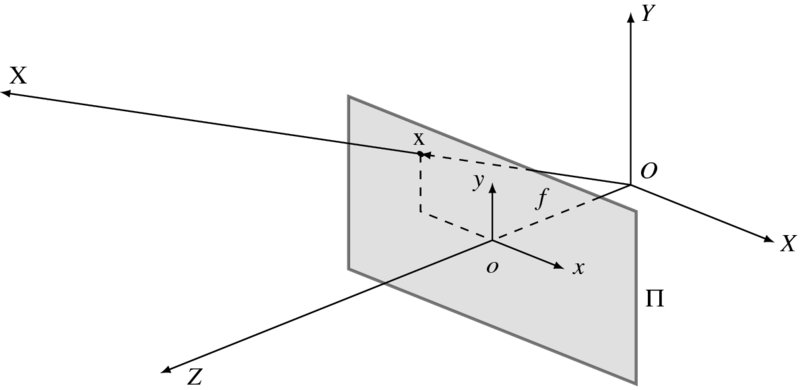
Figure 7.1 A 3D space O and image plane Π (X and x are the object position and image, respectively)
7.1 3D Motion
Visual motion provides three types of information: camera motion, dynamics of the moving objects, and the spatial layout of the scene. To begin with, we consider a 3D space, in which the image plane Π and an object X are defined (Figure 7.1). The world coordinates and the image coordinates are defined by the origins O and o, respectively. The image plane is positioned at (0, 0, f) in this space, where f is the focal length. The vector X is projected onto x in the image plane. When X moves, x does so also in the 2D plane. There is a geometrical relationship between the object motion and the observed velocities. The relationships can be represented in various forms: component, vector, and matrix. In a more general setting, both objects and camera may move, resulting in relative velocities.
In a perspective projection, if a point X = (X, Y, Z)T in 3D space is mapped to a point x = (x, y, f)T in 2D space, the image position is represented by
This is the relationship of the absolute positions (x, y) and (X, Y, Z) in the two spaces. The relationship between differentials ![]() and
and ![]() in the two spaces is sometimes needed.
in the two spaces is sometimes needed.
Note that different matrices are used in transforming the position and velocity from 3D to 2D. In general, the relationship of the coordinates as well as their differentials is nonlinear. Higher-order differentials are involved with even more nonlinear representation.
If the 3D position moves with ![]() , the observed velocity
, the observed velocity ![]() becomes
becomes
If the object is rigid, the motions of the points on the object surface are all dependent. Otherwise, if the object is non-rigid (Vedula et al. 2005), the object points are all independent in their motion. To deal with a non-rigid body, we need a dense three-dimensional vector field defined for every point on every surface in the scene.
For a rigid body's motion, we define the translational and rotational velocities by t = (tx, ty, tz)T and ω = (ωx, ωy, ωz)T. In the world coordinate system, the composite velocity of the object is
In matrix form, the motion vector becomes
which, in component form, is
Combining Equations (7.3) and (7.6), we get
The matrix representation is ![]() :
:
and the vector form is
The motion flow comprises translational and rotational components (Figure 7.2). This figure shows two cases of pure translation, a case of pure rotation, and one of composite motion.
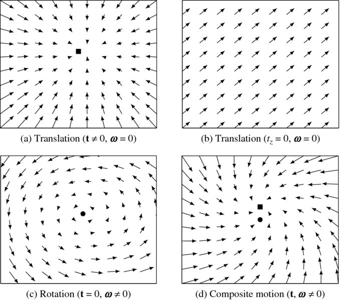
Figure 7.2 Motion fields (FOC, FOE, and AOR are denoted with marks. f = 1 and Z = 10)
Let's represent the composite motion vector by
The first term is a translation component, known up to a scale factor Z, that is t/Z. The second term is a rotational component, which is independent of the depth, Z. If tz ≠ 0, the translational flow field is
where (x0, y0) = (ftx/tz, fty/tz) is the focus of expansion (FOE) (or focus of contraction (FOC)), which is the fixed point of the translational flow field. The translation vector is also related to the time to collision:
which is equivalent to Z/tz.
The motion field is radial with all the vectors pointing towards or away from a single point. The length of the motion field is inversely proportional to the depth. It is also directly proportional to the distance to the FOE. If tz = 0, the translational field is
All motion field vectors are parallel to each other and inversely proportional to depth.
If ωz ≠ 0, the rotational flow field is
which is centered at a fixed point, (fωx/ωz, fωy/ωz), called an axis of rotation (AOR).
Thus far, we have considered a point motion. In many cases, the moving objects may be modeled by a moving plane. Let us consider such a plane, X = (X, Y, Z)T, which has the normal vector n = (nx, ny, nz)T and a distance d from the origin. Then, nT · X = d. Substituting the image point, x = fX/Z, we obtain
Putting this into Equation (7.7), we have the motion field equation:
where
The motion field is the second-order polynomials, where the coefficients are the functions of (n, d, t, ω). That is, the motion field of a planar surface is a quadratic function in the image.
7.2 Direct Motion Estimation
Direct motion estimation is used to recover the 3D motion from the observed image features, without relying on the intermediate variable, optical flow. Because the concept is very intuitive, let us first review this method.
From the outset, we assume the brightness constancy constraint, which will be treated in detail in Section 7.5:
Combining Equations (7.8) and (7.17), we get
We can reduce the variables in this equation by using Equation (7.1):
We have one equation for each pixel, which contains seven variables, (Z, t, ω). There are algorithms that solve this problem, by modeling Z in parameters (Black and Yacoob 1995; Negahdaripour and Horn 1985).
In real-time stereo (Harville et al. 1999), the depth can be measured directly. The depth constraint can then be derived and combined with the brightness constraint. The direct depth method uses the depth data, Z, to model the depth as
which gives the depth constraint,
Note that the constraint is similar to that of brightness. We can derive
Similarly, for the brightness constraint, we obtain
Combining Equations (7.22) and (7.23), we get
Finally, we have
If ∇tI and ∇tZ are available, we can solve this equation for (t, ω).
7.3 Structure from Optical Flow
The other approach is to recover the motion (t, ω) from the given optical flow, (u, v). First, let us estimate t from the optical flow. One of the methods is to minimize the energy:
If we define a = ftx − xtz and b = fty − ytz, the energy function has the form ![]() . We first minimize the sum of least squares with respect to the depth, obtaining Z = (a2 + b2)/(au + bv). Inserting Z into the energy equation, we have
. We first minimize the sum of least squares with respect to the depth, obtaining Z = (a2 + b2)/(au + bv). Inserting Z into the energy equation, we have
If we differentiate this function in terms of tx, ty, and tz, we obtain
where F = (av − bu)/(a2 + b2). The three equations are linearly dependent and difficult to solve.
Therefore, we define a different norm instead:
If we differentiate the function with respect to Z, we get the same Z = (a2 + b2)/(au + bv), but have a simpler energy function,
Differentiating this function with respect to the variables, we have
where
The solution is a singular vector that has the smallest singular value.
For the rotational case, we define
Differentiating with (ωx, ωy, ωz), we have
This can also be solved by LMS or pseudo-inverse.
When the motion field contains both translational and rotational components, we can define the metric:
or, in vector form,
The motion parallax can be assumed because the difference in motion between two very close points does not depend on rotation. This information can be used at depth discontinuities to obtain the direction of translation. For two points,
Therefore,
On the other hand, vector components that are perpendicular to the translational component are due to the rotation.
taking
One of the motion estimation methods is to decompose the motion flow into translational and rotational components. Translational flow field is radial (all vectors emanate from – or pour into – one point), whereas rotational flow field is quadratic in image coordinates. Either search in the space of rotations: remaining flow field should be translational. Translational flow field is evaluated by minimizing deviation from the radial field:
or search in the space of the directions of translation: vectors perpendicular to translation are due to rotation only. Refer to (Burger and Bhanu 1990; Heeger and Jepson 1992; Nelson and Aloimonos 1988; Prazdny 1981).
The other line of research is to use the parametric model for the motion field (Higgins and Prazdny 1980; Waxman 1987). In this approach, the flow is linear in the motion parameters (quadratic or higher order in the image coordinates) and thereby the parametric model for local surface patches (planes or quadrics) solves locally for motion parameters and structure.
7.4 Factorization Method
Given a set of feature tracks, the factorization method estimates the 3D structure and 3D (camera) motion by SVD (Tomasi and Kanade 1992a), using an assumption of orthographic projection.
A general affine camera is represented by the combination of the orthographic projection and the affine transformation of the image:
where A is the projection matrix and b is the translation vector. Let {xij|i ∈ [1, m], j ∈ [1, n]} be the images of the fixed 3D points, {Xj|j ∈ [1, n]}, with m cameras. Considering the affine transformation, the projection is represented by
The problem is to determine m projection matrices A, m vectors b, and n points X, given the mn points x. For the reconstruction, we have 2mn known variables, 8m + 3n − 12 unknowns, and 12 degrees of freedom for the affine transformation:
This equation gives m ≥ 2 and n ≥ 4 in ideal cases. Generally, we need more than four corresponding points:
Let us subtract the centroid of the image points:
We have also the 3D points, subtracted with the centroids. For simplicity, we assume that the origin of the camera and the world coordinate systems are all defined at the centroid of the image points and 3D points:
We build a matrix equation, H = AX:
Here, H is the 2m × n measurement matrix, A is the 2m × 3 motion matrix, and X is the 3 × n structure matrix. Note that the measurement matrix only has rank 3.
The problem becomes one of computing
The usual approach is to decompose the measurement matrix into two matrices with rank 3. First, we use the SVD,
where Λ' is a diagonal matrix that has the eigenvalues sorted along the diagonal. Then, take the first three largest eiegenvalues, λ1 ≥ λ2 ≥ λ3, of Λ' and build the diagonal matrix:
The solution is
The decomposition is not unique, since
where G is any 3 × 3 invertible matrix. To remove this uncertainty, we use the constraint that the image axes are perpendicular and unity. For each camera, Ai = (ai1, ai2)T, find Fi that satisfies
This gives us a large set of equations for the entries in matrix F. Using Cholesky decomposition, we have F = GGT. The solution is then
There are numerous variations of the factorization methods: orthographic (Tomasi and Kanade 1992b), weak perspective (Tomasi and Weinshall 1993), para-perspective (Poelman and Kanade 1994, 1997), sequential factorization (Morita and Kanade 1997), perspective (Sturm and Triggs 1996), factorization with uncertainty (Anandan and Irani 2002), element-wise factorization (Dai et al. 2013), online factorization (Kennedy et al. 2013), and affine factorization (Wang et al. 2013).
7.5 Constraints on the Data Term
Thus far, we have reviewed some issues associated with estimating 3D motion and structures, directly or indirectly, from images. The optical flow is an intermediate variable that behaves like a latent variable in 3D reconstruction. Unlike the 3D quantities, the optical flow is defined on the 2D image and is related to the correspondence problem in two or more image sequences. In this problem, the constraints are the most crucial, together with minimization method, for resolving the uncertainties originating from the ill-posed nature.
To estimate optical flow, we usually build an energy function that consists of data and smoothness terms:
Here, the variable is the optical flow, v. The data term builds a relationship between the data and the estimated variable. The smoothness function states the relationship between neighborhoods in terms of the optical flow. From a physical point of view, the data term is related to the conservation law of brightness or the differential of brightness in time and space. The smoothness term is related with the spatial variation of the estimated variables. The constraint is local in the data term but global in the smoothness term.
The optical flow problem consists of building the energy function, which is a cost function of the variables, and solving it using the optimization method, which is a general optimization technique tailored to the problem. Therefore, the performance to a large extent depends on how the energy function models the problem with efficient constraints. The multitude of algorithms in optical flow largely depends on the diversity of the constraints and the method of optimization. In this section, we review some representative local and global constraints. For an extensive review on optical flow, see (Raudies 2013; Wikipedia 2013b). Let us review in detail the constraints on the data term first.
The starting point of the constraints on the data term is the brightness constancy (BC). The motion analysis needs a stack of video frames, which can be represented as depicted in Figure 7.3. A video signal can be viewed as a stack of images in the direction of the time domain. In the spatiotemporal space, called the motion cube, objects are considered to move in the x-y plane as well as in the t direction. The constraint on motion is the relationship between successive image frames, {I(x, y, t)|t = 0, 1, …}. For the stereo-motion system, the data sequence is the image pairs, ![]() . In this spatiotemporal space, many new features can be defined (Freeman and Adelson 1991; Sizintsev and Wildes 2012).
. In this spatiotemporal space, many new features can be defined (Freeman and Adelson 1991; Sizintsev and Wildes 2012).
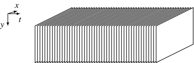
Figure 7.3 A motion cube ( )
)
The optical flow is a generalization of the disparity from 1D to 2D. Therefore, the constraints must also be generalized. As with binocular vision, the corresponding points must have the same intensity, called the photometric constraint. When the optical flow is (u, v), the two points must be equally bright, unless some special illumination is involved. The brightness conservation equation (or image constraint equation) (Fennema and Thompson 1979) is
where the time is normalized to the sampling interval. This is the brightness constancy (BC).
The residual is defined by
which is a generalization of Equation (6.71). This measure assumes that the illumination is constant within the sampling time, and holds even for large variations of optical flow. Because this measure holds for a pixel, it causes the aperture problem to arise. For a pair of pixels, we have one equation with two variables, and thus obtain one vector: the normal. To remove the uncertainty, we build the energy function by integrating the local measure and constraints over the image plane.
The next constraint is the linearized brightness constancy. If the variation in optical flow is small, the BC can be approximated by the Taylor series,
where O(u, v) is the higher-order terms. Taking the first-order Taylor series, we obtain the optical flow constraint equation (OFCE) (Horn and Shunck 1981),
where, v = (u, v)T is the motion vector and ∇t = (∂x, ∂y, ∂t)T is the gradient operator. We simply call this the linearized brightness constancy (LBC). We define the residual by
Although this measure is defined for a small variable, it inherits all the properties of the BC.
Two variables in one equation signify that the equation is under-determined. Using the Moore-Penrose pseudo-inverse, we have v⊥ = −It∇I/|∇I|2. This is just a row-space vector and all the null-space vectors are missing. Any vector having the form v = v⊥ + v∥ satisfies the equation, where ![]() is the unit null-space vector and
is the unit null-space vector and ![]() . This can be interpreted geometrically as follows. In (u, v) space, the equation represents a line. For all vectors on this line v⊥ is unique. In the (u, v) plane, the photometric constraint is represented by a straight line
(Figure 7.4).
Only a normal vector, v, can be estimated with the given photometric constraint. This phenomenon is often called the aperture problem. Viewing in a small window, we can estimate only the normal component of the motion field. This uncertainty can be resolved by constraint propagation between neighborhoods. Hence, the energy function must be an integration of the residuals over the entire image plane.
. This can be interpreted geometrically as follows. In (u, v) space, the equation represents a line. For all vectors on this line v⊥ is unique. In the (u, v) plane, the photometric constraint is represented by a straight line
(Figure 7.4).
Only a normal vector, v, can be estimated with the given photometric constraint. This phenomenon is often called the aperture problem. Viewing in a small window, we can estimate only the normal component of the motion field. This uncertainty can be resolved by constraint propagation between neighborhoods. Hence, the energy function must be an integration of the residuals over the entire image plane.
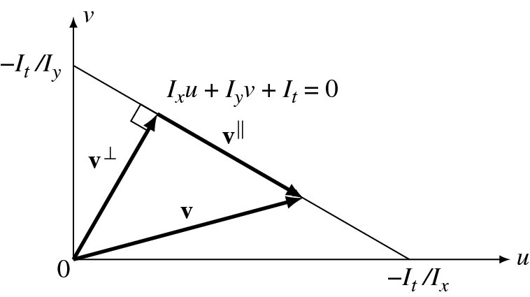
Figure 7.4 Given the photometric constraint, only the normal vector, v⊥, of the true vector, v, can be estimated: v∥ for null vector (The unit null vector:  .)
.)
Even this normal vector cannot be estimated immediately. To see this, consider one-dimensional motion as in depicted Figure 7.5. Assume that an object moves from I(x, t) to I(x, t + 1). To determine the vector v, we need a normal vector and a gradient vector. v0 is obtained at the first iteration. Starting from this intermediate position, the next vector can be obtained. The same process can be repeated until the vector arrives near the second curve, I(x, t + 1). In math expressions, we have
where T is the termination time when the difference (I(x + vk − 1, t + 1) − I(x, t)) is within a small termination condition. The convergence can be enhanced if we use the higher terms in the Taylor series of I(x + u, y + v, t + 1). This iterative approach is used in (Lucas and Kanade 1981).
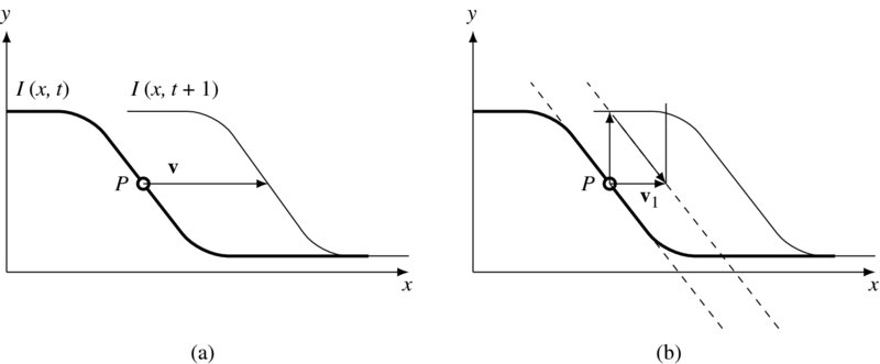
Figure 7.5 Meaning of the photometric constraint: ∇ITv = −It
We can use a local average to expand the LBC to the gradient structure tensor. Multiplying ∇tI on both sides of Equation (7.59), we obtain
The 2 × 2 upper-left submatrix is the Harris operator (Harris and Stephens 1988). If we further apply Gaussian filtering to a small neighborhood, the equation becomes
where ![]() is a template of the Gaussian filter. The matrix is called a motion tensor (or structure tensor). This equation is represented by
is a template of the Gaussian filter. The matrix is called a motion tensor (or structure tensor). This equation is represented by
This constraint is used in (Lucas and Kanade 1981).
The brightness constancy is not always true. If the background illumination is graded, ∇I ≠ 0, it fails. In such a case, we may use the gradient brightness constancy (GBC):
This constraint also may fail for large changes in background illumination.
Several methods exist that assume that higher-order derivatives are conserved (Nagel 1987; Simoncelli 1993; Uras et al. 1989). The constraint is expressed as
Because of the higher-order derivatives, this method tends to be fragile to noise and may lose the information about the first-order deformation. We may also build matrices similar to the structure matrix, by taking local Gaussian filtering.
In a more general environment, the local features can be expanded to the local descriptors (Bay et al. 2006; Calonder et al. 2010; Lowe 2004; Tola et al. 2010), which provide robust and accurate correspondences between images under noisy environments. The correspondence based on the descriptors acts as a concrete matching cue in scenarios with large brightness changes, large motion of small objects, and affine distortions between frames. Define ρ(x, y) to be the matching score for the two descriptors in the current frame and their corresponding descriptors in the next frame, respectively. The descriptor matching term can then be defined as
where δ(x, y) is the indicator variable that is activated when the descriptor is located at (x, y) and ![]() is the correspondence vector from descriptor matching.
is the correspondence vector from descriptor matching.
Similarly to the brightness, we can define phase constancy for the phase. In the frequency domain, the motion reveals a certain conservation law – conservation of phase in each bandpass channel (Fleet and Jepson 1990, 1993; Gautama and van Hulle 2002). Given a complex-valued bandpass channel, r(x, y, t), with phase ϕ(x, y, t), the conservations law is stated as
which is similar to the brightness constancy. We call this the phase constancy (PC). In the first-order Taylor series, this becomes
or in vector notation,
The difficulty is that phase is a multifunction, only uniquely defined on intervals of width 2π, so explicit differentiation is difficult. Instead, the phase derivative is replaced with amplitude derivative (Fleet 1992; Fleet and Jepson 1990):
The phase is amplitude invariant and thus is quite robust to illumination but fragile near occlusion boundaries and fine-scale objects.
7.6 Continuity Equation
One of the universal laws in physics is that of conservation, which is represented by the continuity equation. In computer vision, the brightness, gradient brightness, and phase are the quantities preserved even in space and time variations. If Iv is regarded as a flux, the LBC can be represented by the mass continuity equation:
where ∇ · is divergence. Note that the vector is constrained to ∇v = 0, which means the smoothness constraint, as we will see shortly. In an analogy to fluid dynamics, ∇ · v = 0 means that the divergence of the velocity field is zero everywhere, indicating that the local volume dilation rate is zero. If we consider ∇Iv as a flux, the GBC becomes
The same continuity equation can be applied to the phase. For the phase, we may consider ϕv as a flux. The LPC then becomes
Similarly, for the GPC, the continuity equation becomes
The LBC can be represented by
where ∇t = (∂/∂x, ∂/∂y, ∂/∂t)T. Multiplying ∇t on both sides and convolving with Gaussian filter, we have
The resulting matrix is the structure matrix. This derivation can also be applied to the other variables.
It appears that the various models on the data terms are related to the continuity equation. Moreover, the continuity equations are naturally expanded to color systems such as RGB or HSV. For a detailed review of continuity, refer to (Raudies 2013).
7.7 The Prior Term
In addition to the data term, the prior term in an energy equation is related to various constraints associated with motion mechanics and geometry. These constraints are free from the data but dependent on the nature of the variables in a wider range than the local points. In optimization view, the prior term behaves as a regularizer. The constraints can be classified into isotropic and anisotropic regularizers. The isotropic regularizer applies the constraint uniformly over the image regardless of the object or motion boundary. The anisotropic regularizer, on the other hand, determines the weights and directions depending on the local context.
Let us first review the isotropic smoothness constraints. One of the important constraints on optical flow is the spatial continuity of the optical flow on the surface. The simplest way to represent the spatial smoothness of flow vectors is to favor the following first-order derivatives:
which is the generalization of the disparity from one dimension to two dimensions. The continuity equations assume this constraint.
In the construction of the smoothness energy function from the first-order constraint defined above, a variety of penalty functions are utilized to accurately model the characteristics of flow vectors under complex situations. The energy function based on L2 norm is
The energy function based on L1 is
The prior can be classified into homogeneous and inhomogeneous regularizer. The inhomogeneous regularizers are further classified into image-driven or flow-driven and isotropic or anisotropic (Raudies 2013). The above regularizers are homogeneous according to this classification.
An image-driven isotropic regularizer varies smoothness depending on the image context:
where σ is a parameter. The regularization becomes strong around image discontinuity and weak at the uniform region. There is no directional preference, depending on edge direction (Alvarez et al. 1999).
An image-driven anisotropic regularizer changes smoothness asymmetrically depending on the image context:
where κ is a constant. The smoothing becomes weak at the boundary and strong at the homogeneous region. The smoothing also applies only along the boundary, and not across it.
A flow-driven isotropic regularizer controls the smoothness according to the flow of vectors. The following measure uses a convex function of the vector (Bruhn et al. 2006):
where κ is a constant.
A flow-driven anisotropic regularizer defines the smoothness anisotropically depending on the vector flow (Weickert and Schnorr 2001):
where κ is a constant and tr means trace. See (Raudies 2013) for more details on regularizers.
The motion occlusion is the generalization of the disparity occlusion. When an object moves with v, there appear two undetermined regions to the front, mid, and rear regions of the object. Let an object A move from ![]() to
to ![]() . The front occluding region A(t − 1) − A(t) then appears in I(t), the rear occluding region A(t) − A(t + 1) appears in I(t), and the middle occluding area is the overlapped region, A(t)∪A(t + 1), which exists in both images. The occluding regions – front and rear regions – are the uncertain regions where the optical flow cannot be defined. Detecting the regions is a crucial task in optical flow computation.
. The front occluding region A(t − 1) − A(t) then appears in I(t), the rear occluding region A(t) − A(t + 1) appears in I(t), and the middle occluding area is the overlapped region, A(t)∪A(t + 1), which exists in both images. The occluding regions – front and rear regions – are the uncertain regions where the optical flow cannot be defined. Detecting the regions is a crucial task in optical flow computation.
The occluding region is principally where the optical flow is not defined. However, the occluding region is defined only when the optical flow is assumed. Therefore, most algorithms define an occluding indicator that is a function of optical flow and use it to switch the smoothness term, so that the smoothness term is validated only in the non-occluding region.
Let ρ(x, t) be an occlusion indicator (or detector). The occlusion can be detected by the squared image residue (Xiao et al. 2006):
where ε is a threshold to detect the occlusion. If ρ = 0, the pixel is occluded and if ρ = 1, the pixel is visible in both images. To make the occlusion indicator, it can be approximated by
The optical flow vector can be used to detect occlusions (Sand and Teller 2008; Sand 2006):
The edges and corners in the spatiotemporal domain correspond to the occluded pixels. These points of interest are detected using the minimum eigenvalue of the gradient structure tensor (Feldman and Weinshall 2006, 2008):
where the operators * and G represent convolution and Gaussian kernel, respectively. The operator is invariant to the translation and rotation. The region with higher values of λ tends to be the outline of the object. This operator can be modified to the velocity-adapted occlusion detector (Feldman and Weinshall 2006, 2008):
where G denotes the 2 × 2 upper-left submatrix of the gradient structure tensor.
The Frobenius norm of the gradient of the optical flow field can be used to capture the motion discontinuity (Sargin et al. 2009):
which is helpful to detect occlusion.
The occlusion indicator is usually utilized in controlling the prior term:
Around the occlusion, only the data term operates, the smoothness term is ignored. As a result, the occlusion region is undetermined but the boundaries are accurately preserved.
Another strong constraint for the smoothness term is based on the parametric motion model. The global motion model (Altunbasak et al. 1998; Cremers and Soatto 2005; Odobez and Bouthemy 1995) offers more constrained solutions than smoothness, such as the Horn–Schunck method. It also involves integration over a larger area than a translation-only model can accommodate, such as the Lukas-Kanade method. More specifically, we suppose
where T( · ) is a transformation in 2D or 3D, with parameters a. The possible models are 2D and 3D motion models. The 2D models include translation, affine, quadratic, and homography. The 3D model includes camera motion, homography with epipole, and plane with parallax (Adiv 1985; Hanna 1991; Nir et al. 2008; Valgaerts et al. 2008; Wedel et al. 2008a, 2009).
A quadratic model for the 2D motion is parameterized by
In the projective model, the parameters are
In the 3D motion model, the instantaneous camera motion method assumes the global parameters, ω and t, together with the local parameter, Z(x, y). The motion vector is
The model for homography and epipole uses the global parameters, a1, …, a9, t1, …, t3 and the local parameters: γ(x, y).
There is a method that uses residual planar parallel motion, that also uses the global parameters: a1, a2, a3 and the local parameter γ(x, y).
In addition to constraints, special features have been developed for motion estimation. In space-time, the feature can be either intensity variation (Sizintsev and Wildes 2012) or texture (Derpanis and Wildes 2012), quadric elements (Granlund and Knutssen 1995) or Grammian (Shechtman and Irani 2007). The quantities can be a response from the local filter responses such as Gaussian–Hilbert (Freeman and Adelson 1991), Gabor, and log-normal. For example, Sizintsev et al. proposed Stequel as a quadric weighted by the Gaussian-Hilbert response in icosahedron directions (Jenkins and Tsotsos 1986; Sizintsev and Wildes 2012).
7.8 Energy Minimization
We have reviewed various constraints on the data and prior terms. The energy function consists of both these terms. Therefore there are numerous variations on combinations of the data and smoothness terms. In minimizing the energy function, many optimization methods can be utilized, including baseline methods such as those of Horn and Shunck (Horn and Shunck 1981) and Lukas and Kanade (Lucas and Kanade 1981). Horn's method advocates the LBC and smoothness regularization for the energy function and the variational method for energy minimization. On the other hand, Lukas–Kanade's method uses the gradient structure tensor for the energy function and the LMS method for energy minimization.
A general solution based on the variational method is given by (Horn and Shunck 1981). The energy function is the combination of the LBC and the smoothness function with gradient magnitude:
Let E = ∫F(u, v, ux, uy, vx, vy)dxdy and derive the Euler–Lagrange equations,
Inserting F, this becomes
Let the local average
and the Laplacian
Then, the equations become
Solving this, and taking iterative forms, we have the equations,
The computational structure is suitable for the Gauss–Seidel or Jacobi methods. This can be efficiently realized with the relaxation, DP, and BP architectures, introduced in Chapters 8 through 10.
The other general solution based on LMS is given by (Lucas and Kanade 1981), which uses the gradient structure tensor. For a point, Equation (7.59) becomes
The pseudo-inverse is
For a point, we have one equation and two variables. The solution is the normal flow, v⊥, as observed in the aperture problem.
To get more equations for a pixel, impose additional constraints by assuming that the flow field is smooth locally, and thus the neighbors have the same optical flow. Consequently, we obtain, Av = −It:
Usually, A is a local weighted sum of intensity with a Gaussian function. This can be represented by the Gaussian kernel, W = {wij|i, j ∈ [1, n]}:
In component form, this is
This system is over-determined and thus can be solved by LLSE. If ATW A is invertible, we have
In general, the brightness constancy is not satisfied, the motion is not small, a point does not move like its neighbors, and thus, the LMS method is not satisfactory. The enhanced method is the iterative Lukas–Kanade method (Kanade 1987; Lucas and Kanade 1981).
7.9 Binocular Motion
When objects are observed with a stereo camera, the image frames contain both stereo and motion information, for example disparity and optical flow. Let us consider the case depicted in Figure 7.6, in which the origins Ol and Or are, respectively, the projective centers of the left and right images, Ilt and Irt; the image planes are coplanar and the optical axes are parallel, separated by a baseline B. In this setting, a point P = (X, Y, Z)T moving from P to Q is projected onto the two image planes as pl = (xl, yl)T and pr = (xr, yr)T. This alignment is parallel optics, and the epipolar lines, on which corresponding points are located, are the same for both images.
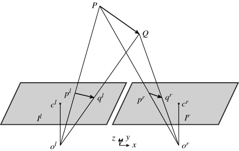
Figure 7.6 Projection of moving object
Two images of the same size, M × N, are captured at constant intervals in time t. In 3-space, the point P is generally moving with a velocity V = (U, V, W)T, where (U, V, W) describes the translation components. Accordingly, the two projected points also move on the image planes with the optical flows, vl = (ul, vl) and vr = (ur, vr). Furthermore, the two projected points are separated with the disparity, d, on both image planes. (Incidentally, the rotational movement is omitted to make the problem simple.) If the sampling rate is fast enough or, equivalently, the rotation is slow enough, this assumption is correct even for the general case.
From Equation (7.7), we have
Likewise, the disparity–depth relation becomes
Taking the time derivative of both sides, we obtain
Substituting Equation (7.113) into Equation (7.111) yields the equation
The first equation specifies that the difference between the two optical flows is identical to the difference between the two disparities. The second equation is due to the epipolar assumption: the corresponding points are on the same epipolar line whenever the point moves. This equation means that there are five variables in two equations and explains the relationship between disparity and optical flow, bypassing the 3D positions and velocity.
The combination of motion and stereo can be explained by the two frames of stereo images, {Il(x, y, t), Ir(x, y, t), Il(x, y, t + 1), Ir(x, y, t + 1)}. In this system, we assume that d(x, y, t) = d0(x, y, t) is known. Then, for the unknowns, (vl, vr, d), the following constraints hold:
The first two equations are the brightness constraints for the stereo matching. The next two constraints are the relationships between disparity and optical flow. The last two equations are the linearized brightness constraints for the optical flow. For the four points, we have four equations and five variables.
The constraint equations are drawn in Figure 7.7. Unlike Figure 7.4, two lines characterize the (u, v) plane. The equation, vl − vr = 0, appears as a vertical line in this graph and the resulting crossing points define (ul, ur). However, the position of the vertical line is defined by ![]() , the vertical separation between the two lines. Hence, if
, the vertical separation between the two lines. Hence, if ![]() is decided, via stereo matching, vl and vr are all determined uniquely. Since there is no other constraint on the two lines except a negative slope, degenerate cases exist. The typical case is when the two lines are parallel to each other. In this case, even though the separation
is decided, via stereo matching, vl and vr are all determined uniquely. Since there is no other constraint on the two lines except a negative slope, degenerate cases exist. The typical case is when the two lines are parallel to each other. In this case, even though the separation ![]() is known, no single vl = vr is defined. The degenerate case occurs when the slopes of the two lines are the same: Ily/Ixl = Iry/Ixr. The worst case occurs when the two lines are overlapping, that is Ilx = Ixr and Ily = Iyr. We may solve this problem by the variational method or the LMS method (Jeong et al. 2012).
is known, no single vl = vr is defined. The degenerate case occurs when the slopes of the two lines are the same: Ily/Ixl = Iry/Ixr. The worst case occurs when the two lines are overlapping, that is Ilx = Ixr and Ily = Iyr. We may solve this problem by the variational method or the LMS method (Jeong et al. 2012).
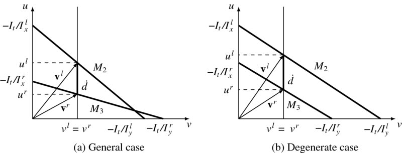
Figure 7.7 The relationships between  and (vl, vr)
7.10 Segmentation Prior
The determination of disparity and optical flow is generally aided by image segmentation. This concept can be generalized to the segmentation, which involves many attributes of the image. The segmentation, whether it is defined for regions or edges, is usually the final goal of the early vision. Using this method, regions classified as having the same label tend to be assigned with the same disparity or optical flow. This segment-based constraint, if available, can help the smoothness constraint to retain the sharp boundaries. The reason is that the pixels defined inside the segments or contours are similar with respect to some characteristic but the pixels in adjacent regions or across contours are significantly different with respect to the same characteristics. The result of segmentation can be easily integrated into the energy functions in higher level vision, in the form of constraint terms or initial values of the labeling. However, the segment characteristics such as brightness, color, texture, and edges and the high level characteristics such as surface orientation, disparity, optical flow, or object class may not always coincide. Some of the typical methods are thresholding, edge detection, histogram, compression-based, region growing, clustering, split-and-merge, model-based method, graph partitioning, and multi-scale methods.
One of the practical segmentation methods is soft matting (Levin et al. 2007, 2008, 2011; Shi and Malik 2000; Sun et al. 2010), which can be easily ported to the disparity and optical flow. In this method, the matting Laplacian matrix (Levin et al. 2008) is
where Ii and Ij are the colors of the input image at pixels i and j, δij is the Kronecker delta, μk and Σk are the mean and covariance matrix of the colors in window Nk, I3 is a 3 × 3 identity matrix, ε is a regularization parameter, and |Nk| is the number of pixels in window Nk.
We can consider the Laplacian matrix as a quadratic approximation of exponential form:

Furthermore, omitting the ε term and generalizing the correlation term yields
The segmentation result using Lk can be added to the smoothness constraint in the energy equation, so that the same segment may be assigned with the same labels.
7.11 Blur Diameter
Thus far, we have examined stereo vision and motion estimation, estimating depth, motion, structure, and camera pose. Now we examine some of other modalities in vision that are associated with depth estimation. The intrinsic parameters explain the pixels, focal length, and possibly the lens distortion. What is missing is the effect of real aperture, which generates unequal sharpness, called blurring, across the image plane. At one end, this unequal focusing is regarded as undesirable and must be rectified by inverse filtering. At the other end, except for artistic effect such as portrait photographing, the defocusing is considered as an encoding process of depth information, such that the degree of blur is in proportion to the depth. The amount of blur can be represented by the blur diameter of the PSF. Like the disparity or optical flow, the blur diameter can be estimated and used for depth computation.
Suppose that there is a typical lens system, such as that drawn in Figure 7.8, which is called a thin lens system. In this figure, P1 and P2 are the principal planes, and Q1 and Q2 are the principal points. A lens with focal length f is focused on a scene point P at a subject distance r0, and this focused point is mapped to r' on the image plane. A point other than the subject distance is mapped to z' and thus defocused, as indicated by the blur diameter 2R.
For a point, P, this system satisfies
For a point, P, the defocused image satisfies
These equations express the fact that a point between the lens and P is focused in front of the image plane, whereas a point behind P is focused behind the image plane. In either case, the projected image will appear as a spot with radius R of the circle of confusion (or blur circle), on the image plane.
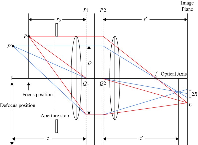
Figure 7.8 The camera optics with thin convex lens
Comparing the two triangles, one on either side of f, we can derive a relationship between the blur radius R and the distance z':
Using r' in Equation (7.119) and z' in Equation (7.120), we have
For the case where r0 ≫f and |z − r0| are not negligible, Equation (7.122) becomes
Once R is known, we can obtain the object distance from the blur disk:
We have observed that, like disparity and optical flow, the blur diameter is another measure that can be obtained from images. If the imaging system consists of compound lenses, the blur–depth relationship becomes a complicated nonlinear system, although the depth is still related with the blur diameter. Blur estimation has been studied in areas such as depth from focus (DfF) (Grossmann 1987; Jing and Yeung 2012) and depth from defocus (DfD) (Li et al. 2013; Subbarao and Surya 1994).
7.12 Blur Diameter and Disparity
Similar to disparity and optical flow giving measures on depth, the blur diameter provides the same measure of depth. It would therefore be useful if the three quantities could be linked in such a way that the common depth quantity is eliminated and the variables are linked directly. In this light, let us first consider linking disparity and blur diameter (Ito et al. 2010; Schechner and Kiryati 2000; Subbarao et al. 1997).
If we substitute Z = fB/d into (7.124) to remove Z, we obtain
This equation links disparity and blur diameter directly, without intervention of the depth, and has the following properties. In a normalized system, this equation has the form ![]() , where the three quantities,
, where the three quantities, ![]() ,
, ![]() , and
, and ![]() , are the normalized values with respect to the baseline, lens diameter, and the image plane distance, respectively. The variables are the disparity and the blur diameter. The two variables have opposite properties in terms of addition: if one decreases, the other increases equivalently, maintaining the total sum at a constant.
, are the normalized values with respect to the baseline, lens diameter, and the image plane distance, respectively. The variables are the disparity and the blur diameter. The two variables have opposite properties in terms of addition: if one decreases, the other increases equivalently, maintaining the total sum at a constant.
It is convenient to generalize R so that it can be either positive or negative depending on the distance r' − z'. Substituting Z for r0 in Equation (6.66) yields
With this and Equation (7.122), we obtain
The d–R curve is drawn in Figure 7.9. Here, the x-intercept is the position where the object is at infinity and the y-intercept is the position where the object is focused. The negative diameter means that the object is focused behind the image plane.
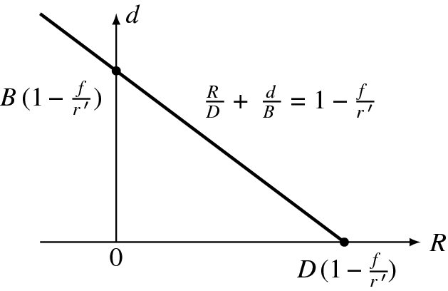
Figure 7.9 The d–R curve
This relationship can be used as a constraint for determining disparity, given blur diameter:
Note that this constraint holds for a pixel, similar to the data term.
7.13 Surface Normal and Disparity
In other vision modules such as shading, texture, and silhouette, the major estimated quantity is the surface normal. Considering the depth (x, y, Z(x, y)), we have the surface normal (Horn 1986):
where (p, q) is the gradient,
The surface normal can be represented by a more versatile vector, called stereographic projection (Horn 1986).
If a surface is sloped, the slope affects both the surface normal and the disparity (Figure 7.10). At (xl, yl), the surface depth is Z(x, y) and the disparity is d(xl, yl). At (xl + Δxl, yl + Δyl), the depth changes by ΔZ and the disparity changes by Δd. If the surface is fronto-parallel, the depth and the disparity are both constant.
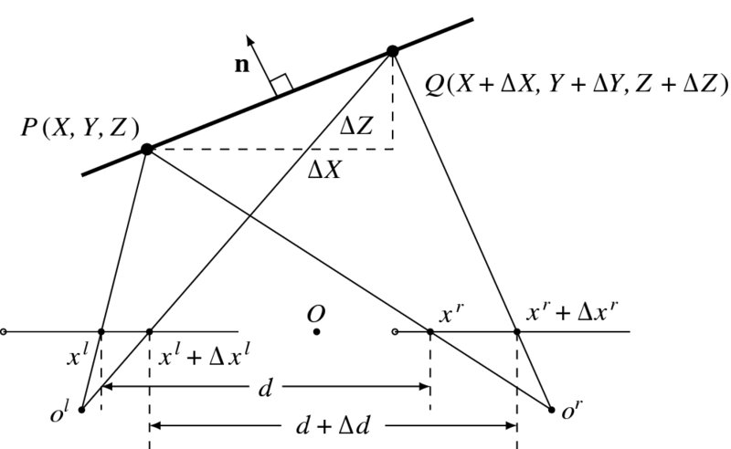
Figure 7.10 The relationship between disparity and surface normal (n: surface normal and d: disparity)
To obtain the relationship between the disparity and the surface slope, we substitute Equation (6.66) into Equation (7.130) and obtain
which is, in fact, p = fB∂xd− 1 and q = fB∂yd− 1. Here, the normal vector and the disparity are all defined in the image coordinates. These identities represent the direct relationship between the disparity and the surface orientation, all in the image plane. If (p, q) is given, these equations can be used as constraints in stereo matching (and vice versa):
Here the distance between neighbors is assumed to be unity.
The surface normal is often estimated with a surface model. If the surface is planar, Z(x, y) = ax + by + c, we have the constraints, dx = −d2a/fB, dy = −d2b/fB. As a special case, if the surface is a fronto-parallel plane, the disparity is constant. For a quadratic model of the surface, Z(x, y) = ax2 + by2 + cxy + d, the disparity becomes dx = ax + cy, dy = by + cx.
If (p, q) ≠ 0, these equations can be further combined into one:
This equation means that the two normals, n = ( − p, −q, 1)T and d = ( − dx, −dy, 1)T, exist in the same vertical plane, that is ![]() . This equation can also be used as a constraint to the smoothness terms.
. This equation can also be used as a constraint to the smoothness terms.
7.14 Surface Normal and Blur Diameter
We may link the blur diameter and the surface normal. This can be achieved by substituting Equation (7.124) into Equation (7.130). The result is
These equations directly link the surface normal to the blur diameter. They can be combined to give
This equation means that the two normals, n = ( − p, −q, 1)T and d = ( − Rx, −Ry, 1)T, exist in the same vertical plane, that is ![]() .
.
The relationship of the surface normal to the blur diameter is illustrated in Figure 7.11. On the left image, the slope ΔZ appears as a prolonged dr, which affects the degree of blur.
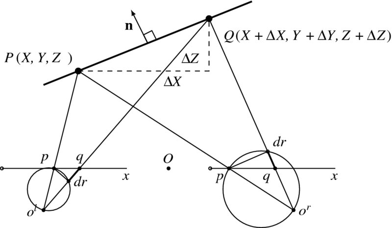
Figure 7.11 The relationship between surface normal and blur diameter (n: surface normal)
For a stereo system, the surface slope influences the blur diameter on both images, as shown in the figure. On the right image, the slope appears as a shortened dr and is represented in Equation (7.124). Unlike other measures, the blur diameters are defined separately in the two images. This results in another relationship: blur difference in two images. This means that more than two modules can be described. In this particular case, disparity, surface normal, and blur diameters are involved.
To obtain the relationship between the blur diameter and the disparity, we insert Equation (7.131) into (7.134) to get
For the functions, R(x, y) and d(x, y), this equation means that the two normals, R = ( − Rx, −Ry, 1)T and d = ( − dx, −dy, 1)T, exist in the same vertical plane: ![]() . We have two sets of equations, Equations (7.125) and (7.136). In one equation, the variables are directly related in a linear equation, and in the other the variables are related in the ratio of differentials.
. We have two sets of equations, Equations (7.125) and (7.136). In one equation, the variables are directly related in a linear equation, and in the other the variables are related in the ratio of differentials.
7.15 Links between Vision Modules
There are vision modules for depth estimation such as depth from defocus (DfD), shape from shading (SfS) (Harrison and Joseph 2012), shape from texture (SfT), shape from contour or silhouette (SfC), as well as stereo vision and motion vision. Integration of vision modules can be achieved by combining them in an energy equation and minimizing it to achieve the best depth. The other approach is to treat the vision modules as weak classifiers and build a combined classifier with boosting methods. It is evident that this integration is limited since the interacting mechanisms between modules are ignored. Eventually, one must look into the tighter relationships between variables defined in different modules.
Thus far, we have examined the constructs for depth estimation: disparity, optical flow, blur diameter, and surface orientation. The relationship between the 2D and 3D variables are summarized in Table 7.1.
Table 7.1 The 2D and 3D quantities
| Measures | Depth | Velocity | |
| Disparity | d | ||
| Optical flow | (u, v) | ||
| Surface normal | (p, q) | ||
| Blur diameter | R |
cf. f: focal length, B: baseline, D: lens diameter, r0: subject distance, and r': image distance.
The 2D quantities are obtained by various vision modules, as stated. Given the 2D quantities, the 3D variables (depth and velocity) can be obtained using the formula in the table. In this formula, we assume the simplest models possible to avoid complexity. In stereo vision, the epipolar rectified system is assumed. For a convergent system, the 3D quantities must be transformed with the projective matrix, which were used in the rectification process. In addition, the aperture system is assumed to be the thin lens system. The disparity and blur diameter give depth in absolute values whereas the surface normal gives only the orientation of the surface. In velocity computation, the quasi-orthographic projection and the small velocity in the Z direction are assumed, and the rotational velocity ignored. For a more general system, we have to replace the equations with more accurate ones.
To remove the 3D variables, the 2D variables can be combined in various ways. The resulting equation gives the direct relationship between the 2D variables, bypassing the 3D variables. Table 7.2 summarizes the relationships between the 2D variables.
Table 7.2 The relationships between 2D variables
| d | (u, v) | (p, q) | R | |
| d | − | 
|

|
|
| (u, v) | − | − | − | − |
| (p, q) | qdx = pdy | − | − | 
|
| R | Rxdy = Rydx | − | qRx = pRy | − |
cf. (p, q): the surface gradient, (dx, dy): the disparity gradient, and (Rx, Ry): the gradient of blur diameter.
The upper triangle is filled with the ordinary equations and the lower triangle is filled with differential equations. Among others, the disparity–normal relationship has the significant meaning that it links the stereo with other modules that provide surface orientation, such as shading, texture, and contour. This table is complete in the sense that the relationships for the optical flow–surface normal and optical flow–blur cannot be obtained without introducing the 3D variables. Because the optical flow is related to (U, V, W) in addition to Z, the blur or surface normal cannot remove all of these four variables. The common properties of the three normals for Z(x, y), d(x, y), and R(x, y) are all positioned in the same vertical plane.
The equations in Table 7.2 are defined between two vision variables. It is possible that three or more variables are linked together. One set of equations is
The other set of equations is
In these equations, the optical flow is missing (see the problems at the end of this chapter). If the optical flow is included also, Equations (7.137) and (7.138) become one or more integro-differential equations, such as
which we call the fundamental equation (FE). The equations in Table 7.2 and Equations (7.137) and (7.138) are all special cases of this integrated equation.
Thinking about interaction between two or more vision modules might give insight into understanding human visual perception. As remarked in Chapter 5, the vision problem can be considered as the minimization of the free energy. If the vision modules work simultaneously, the free energy is composed of FE, together with the ordinary data term and the smoothness term. There is evidence that the human visual system is organized in a systematic manner, such as modules and hierarchy (Bear et al. 2007; Purves 2008; Hubel 1988). It is now necessary to investigate the relationships between vision modules, instead of treating them as independent modules, and integrating them afterward to obtain the best common variables, such as structures and poses. The constraints for the linked variables are much stronger than the constraints when the modules are treated independently and integrated only for their results. Beyond vision, there is the area of multisensory integration (Wikipedia 2013a), in which multimodal integration is studied, so that the information from the different sensory modalities, such as sight, sound, touch, smell, self-motion, and taste, may be integrated.
Problems
- 7.1 [3D motion] An airplane at height L is moving with constant velocity v towards the image plane. Derive a formula that determines the time to collision by observing the projected image. Use the focal length f for the camera.
- 7.2 [3D motion] Prove the following. If another plane has the direction, n = t/|t|, and rotates in ω + n × t, then the two planes have the same motion field.
- 7.3 [Direct motion] Derive Equation (7.22).
- 7.4 [Binocular motion] Expand Equation (7.114) to the general case where the system is not rectified but the motion is still translational.
- 7.5 [Surface normal and blur diameter] Prove that n and ( − dx, −dy, 1) are in the same vertical plane.
- 7.6 [Blur diameter and disparity] Prove that the two vectors, ( − Rx, −Ry, 1)T and ( − dx, −dy, 1)T, are in the same vertical plane.
- 7.7 [Vision modules] Using Equation (7.131), derive an equation that holds for the three 2D variables: surface normal, disparity, and blur diameter.
- 7.8 [Vision modules] Using Equation (7.134), derive an equation that holds for the three 2D variables: surface normal, disparity, and blur diameter.
- 7.9 [Vision modules] Derive an equation containing all three variables: disparity, surface normal, and blur diameter.
- 7.10 [Vision modules] How can the optical flow be linked to the other 2D variables?
References
- Adiv G 1985 Determining three-dimensional motion and structure from optical flow generated by several moving objects. IEEE Trans. Pattern Anal. Mach. Intell. 7(4), 384–401.
- Altunbasak Y, Eren PE, and Tekalp AM 1998 Region-based parametric motion segmentation using color information. Graphical models and image processing 60(1), 13–23.
- Alvarez L, Esclarin J, Lefebure M, and Sanchez J 1999 A PDE model for computing the optical flow Proc. XVI congreso de ecuaciones diferenciales y aplicaciones, pp. 1349–1356.
- Anandan P and Irani M 2002 Factorization with uncertainty. International Journal of Computer Vision 49(2-3), 101–116.
- Baker S, Scharstein D, Lewis JP, Roth S, Black MJ, and Szeliski R 2011 A database and evaluation methodology for optical flow. International Journal of Computer Vision 92(1), 1–31.
- Barron JL, Fleet DJ, and Beauchemin SS 1994 Performance of optical flow techniques. International Journal of Computer Vision 12(1), 43–77.
- Bay H, Tuytelaars T, and Van Gool L 2006 SURF: Speeded up robust featuresComputer Vision–ECCV 2006 Springer pp. 404–417.
- Bear M, Conners B, and Paradiso M 2007 Neuroscience: Exploring the Brain third edn. Williams & Wilkins, Baltimore.
- Black MJ and Yacoob Y 1995 Tracking and recognizing rigid and non-rigid facial motions using local parametric models of image motion Computer Vision, 1995. Proceedings, Fifth International Conference on, pp. 374–381IEEE.
- Bruhn A, Weickert J, Kohlberger T, and Schnorr C 2006 A multigrid platform for real-time motion computation with discontinuity-preserving variational methods. International Journal of Computer Vision 70(3), 257–277.
- Burger W and Bhanu B 1990 Qualitative understanding of scene dynamics for mobile robots. International Journal of Robotics Research 9(6), 74–90.
- Calonder M, Lepetit V, Strecha C, and Fua P 2010 Brief: Binary robust independent elementary features Computer Vision–ECCV 2010 Springer pp. 778–792.
- Cech J, Sanchez-Riera J, and Horaud R 2011 Scene flow estimation by growing correspondence seeds Computer Vision and Pattern Recognition (CVPR), 2011 IEEE Conference on, pp. 3129–3136IEEE.
- Cremers D and Soatto S 2005 Motion competition: A variational approach to piecewise parametric motion segmentation. International Journal of Computer Vision 62(3), 249–265.
- Dai Y, Li H, and He M 2013 Projective multiview structure and motion from element-wise factorization. IEEE Trans. Pattern Anal. Mach. Intell. 35(9), 2238–2251.
- Derpanis K and Wildes R 2012 Spacetime texture representation and recognition based on a spatiotemporal orientation analysis. IEEE Trans. Pattern Anal. Mach. Intell. 34(6), 1193–1205.
- (ed. Purves D) 2008 Neuroscience fourth edn. Sinaur Associates.
- Faugeras O and Luong Q 2004 The Geometry of Multiple Images: The Laws That Govern the Formation of Multiple Images of a Scene and Some of Their Applications. MIT Press.
- Feldman D and Weinshall D 2006 Motion segmentation using an occlusion detector Workshop on Dynamical Vision, pp. 34–47.
- Feldman D and Weinshall D 2008 Motion segmentation and depth ordering using an occlusion detector. IEEE Trans. Pattern Anal. Mach. Intell. 30(7), 1171–1185.
- Fennema C and Thompson W 1979 Velocity determination in scenes containing several moving objects. Computer Graphics and Image Processing 9(9), 301–315.
- Fleet D and Weiss Y 2006 Optical flow estimation Handbook of Mathematical Models in Computer Vision Springer pp. 237–257.
- Fleet DJ 1992 Measurement of Image Velocity. Kluwer.
- Fleet DJ and Jepson AD 1990 Computation of component image velocity from local phase information. International Journal of Computer Vision 5(1), 77–104.
- Fleet DJ and Jepson AD 1993 Stability of phase information. IEEE Trans. Pattern Anal. Mach. Intell. 15(12), 1253–1268.
- Freeman WT and Adelson EH 1991 The design and use of steerable filters. IEEE Trans. Pattern Anal. Mach. Intell. 13(9), 891–906.
- Gautama T and van Hulle MM 2002 A phase-based approach to the estimation of the optical flow field using spatial filtering. IEEE Trans. Neural Networks 13(5), 1127–1136.
- Granlund G and Knutssen H 1995 Signal Processing for Computer Vision. Kluwer.
- Grossmann P 1987 Depth from focus. Pattern Recognition Letters 5(1), 63–69.
- Hanna K 1991 Direct multi-resolution estimation of ego-motion and structure from motion Visual Motion, 1991, Proceedings of the IEEE Workshop on, pp. 156–162.
- Harris C and Stephens MJ 1988 A combined corner and edge detector Alvey Conference, pp. 147–152.
- Harrison AP and Joseph D 2012 Maximum likelihood estimation of depth maps using photometric stereo. IEEE Trans. Pattern Anal. Mach. Intell. 34(7), 1368–1380.
- Hartley R and Zisserman A 2004 Multiple View Geometry in Computer Vision. Cambridge University Press.
- Harville M, Rahimi A, Darrell T, Gordon G, and Woodfill J 1999 3D pose tracking with linear depth and brightness constraints Computer Vision, 1999. The Proceedings of the Seventh IEEE International Conference on, vol. 1, pp. 206–213 IEEE.
- Heeger DJ and Jepson AD 1992 Subspace methods for recovering rigid motion I: Algorithms and implementation. International Journal of Computer Vision 7(2), 95–117.
- Higgins HCL and Prazdny K 1980 The interpretation of a moving retinal image. Proceedings of Royal Society of London B-208, 385–397.
- Horn B and Shunck B 1981 Determining optical flow. Artificial Intelligence 17(1-3), 185–203.
- Horn BKP 1986 Robot Vision. MIT Press, Cambridge, Massachusetts.
- Hubel D 1988 Eye, Brain, and Vision. W H Freeman & Co, http://hubel.med.harvard.edu/index.html.
- Huguet F and Devernay F 2007 A variational method for scene flow estimation from stereo sequences Computer Vision, 2007. ICCV 2007. IEEE 11th International Conference on, pp. 1–7IEEE.
- Ito M, Takada Y, and Hamamoto T 2010 Distance and relative speed estimation of binocular camera images based on defocus and disparity information PCS, pp. 278–281. IEEE.
- Jenkins M and Tsotsos J 1986 Applying temporal constraints to the dynamic stereo problem. Journal of Computer Vision, Graphics, and Image Processing 3358, 16–32.
- Jeong H, Yan S, and Han SH 2012 Integrating stereo disparity and optical flow by closely-coupled method. Journal of Pattern Recognition Research 7(1), 175–187.
- Jing BZ and Yeung DS 2012 Recovering depth from images using adaptive depth from focus ICMLC, pp. 1205–1211. IEEE.
- Kanade T 1987 Three-Dimensional Machine Vision. Kluwer.
- Kennedy R, Balzano L, Wright SJ, and Taylor CJ 2013 Online algorithms for factorization-based structure from motion. CoRR abs/1309.6964, on revision.
- Levin A, Fergus R, Frédo D, and Freeman W 2007 Image and depth from a conventional camera with a coded aperture ACM SIGGRAPH 2007 papers SIGGRAPH '07. ACM, New York, NY, USA.
- Levin A, Lischinski D, and Weiss Y 2008 A closed-form solution to natural image matting. IEEE Trans. Pattern Anal. Mach. Intell. 30(2), 228–242.
- Levin A, Weiss Y, Durand F, and Freeman WT 2011 Understanding blind deconvolution algorithms. IEEE Trans. Pattern Anal. Mach. Intell. 33(12), 2354–2367.
- Li C, Su S, Matsushita Y, Zhou K, and Lin S 2013 Bayesian depth-from-defocus with shading constraints CVPR, pp. 217–224. IEEE.
- Li R and Sclaroff S 2008 Multi-scale 3D scene flow from binocular stereo sequences. Computer vision and image understanding 110(1), 75–90.
- Liu F and Philomin V 2009 Disparity estimation in stereo sequences using scene flow. BMVC, vol. 1, p. 2.
- Lowe D 2004 Distinctive image features from scale-invariant keypoints. International Journal of Computer Vision 60(2), 91–110.
- Lucas BD and Kanade T 1981 An iterative image registration technique with an application to stereo vision. Image Understanding Workshop, pp. 121–130.
- McCane B, Novins K, Crannitch D, and Galvin B 2001 On benchmarking optical flow. Computer Vision and Image Understanding 84(1), 126–143.
- Middlebury 2013 Middlebury optical flow home page http://vision.middlebury.edu/flow/ (accessed Dec. 23, 2013).
- Morita T and Kanade T 1997 A sequential factorization method for recovering shape and motion from image streams. IEEE Trans. Pattern Anal. Mach. Intell. 19(8), 858–867.
- Nagel HH 1987 On the estimation of optical flow: Relations between different approaches and some new results. Artificial Intelligence 33, 299–324.
- Negahdaripour S and Horn BK 1985 Determining 3D motion of planar objects from image brightness patterns. IJCAI, pp. 898–901.
- Nelson RC and Aloimonos Y 1988 Finding motion parameters from spherical flow fields (or the advantages of having eyes in the back of your head). Biological Cybernetics 58, 261–273.
- Nir T, Bruckstein AM, and Kimmel R 2008 Over-parameterized variational optical flow. International Journal of Computer Vision 76(2), 205–216.
- Odobez JM and Bouthemy P 1995 Robust multiresolution estimation of parametric motion models. Journal of visual communication and image representation 6(4), 348–365.
- Poelman CJ and Kanade T 1994 A paraperspective factorization method for shape and motion recovery. Lecture Notes in Computer Science 800, 97–110.
- Poelman CJ and Kanade T 1997 A paraperspective factorization method for shape and motion recovery. IEEE Trans. Pattern Anal. Mach. Intell. 19(3), 206–218.
- Pons JP, Keriven R, and Faugeras O 2007 Multi-view stereo reconstruction and scene flow estimation with a global image-based matching swith. International Journal of Computer Vision 72(2), 179–193.
- Prazdny K 1981 Determining the instantaneous direction of motion from optical flow generated by a curvilinearly moving observer Image Understanding Workshop, pp. 14–21.
- Raudies F 2013 Optic flow http://www.scholarpedia.org/article/Optic_flow (accessed on Dec. 8, 2013).
- Sand P and Teller S 2008 Particle video: Long-range motion estimation using point trajectories. International Journal of Computer Vision 80(1), xx–yy.
- Sand PPM 2006 Long-range Video Motion Estimation Using Point Trajectories PhD thesis MIT, Dept. of Electrical Engineering and Computer Science.
- Sargin ME, Bertelli L, Manjunath BS, and Rose K 2009 Probabilistic occlusion boundary detection on spatio-temporal lattices ICCV, pp. 560–567. IEEE.
- Schechner YY and Kiryati N 2000 Depth from defocus vs. stereo: How different really are they?. International Journal of Computer Vision 39(2), 141–162.
- Shechtman E and Irani M 2007 Space-time behavior-based correlation-or-how to tell if two underlying motion fields are similar without computing them?. IEEE Trans. Pattern Anal. Mach. Intell. 29(11), 2045–56.
- Shi J and Malik J 2000 Normalized cuts and image segmentation. IEEE Trans. Pattern Anal. Mach. Intell. 22(8), 888–905.
- Simoncelli EP 1993 Distributed analysis and representation of visual motion Ph.D.
- Sizintsev M and Wildes R 2012 Spatiotemporal stereo and scene flow via stequel matching. IEEE Trans. Pattern Anal. Mach. Intell. 34(6), 1206–1219.
- Sturm PF and Triggs B 1996 A factorization based algorithm for multi-image projective structure and motion ECCV, pp. II:709–720.
- Subbarao M and Surya G 1994 Depth from defocus: A spatial domain approach. International Journal of Computer Vision 13(3), 271–294.
- Subbarao M, Yuan T, and Tyan J 1997 Integration of defocus and focus analysis with stereo for 3D shape recoveryIn Proc. SPIE Three Dimensional Imaging and Laser-Based Systems for Metrology and Inspection iii, vol. 3204, pp. 11–23.
- Sun J, He K, and Tang X 2010 Single image haze removal using dark channel priors. US Patent App. 12/697,575.
- Tola E, Lepetit V, and Fua P 2010 Daisy: An efficient dense descriptor applied to wide-baseline stereo. IEEE Trans. Pattern Anal. Mach. Intell. 32(5), 815–830.
- Tomasi C and Kanade T 1992a The factorization method for the recovery of shape and motion from image streams Image Understanding Workshop, pp. 459–472.
- Tomasi C and Kanade T 1992b Shape and motion from image streams under orthography: a factorization method. International Journal of Computer Vision 9, 137–154.
- Tomasi C and Weinshall D 1993 Linear and incremental acquisition of invariant shape models from image sequences ICCV, pp. 675–682.
- Ullman S 1979 The Interpretation of Visual Motion. MIT Press.
- Uras S, Girosi F, Verri A, and Torre V 1989 A computational approach to motion perception. Biological Cybernetics 60, 79–87.
- Valgaerts L, Bruhn A, and Weickert J 2008 A Variational Model for the Joint Recovery of the Fundamental Matrix and the Optical Flow vol. 5096 of Lecture Notes in Computer Science. Springer Berlin Heidelberg.
- Vedula S, Rander P, Collins R, and Kanade T 2005 Three-dimensional scene flow. IEEE Trans. Pattern Anal. Mach. Intell. 27(3), 475–480.
- Wang G, Zelek JS, Wu QMJ, and Bajcsy R 2013 Robust rank-4 affine factorization for structure from motion WACV, pp. 180–185. IEEE Computer Society.
- Waxman AM 1987 An image flow paradigm RCV87, pp. 145–168.
- Wedel A, Brox T, Vaudrey T, Rabe C, Franke U, and Cremers D 2011 Stereoscopic scene flow computation for 3D motion understanding. International Journal of Computer Vision 95(1), 29–51.
- Wedel A, Pock T, Braun J, Franke U, and Cremers D 2008a Duality TV-L1 flow with fundamental matrix prior Image and Vision Computing New Zealand, 2008. IVCNZ 2008. 23rd International Conference, pp. 1–6.
- Wedel A, Pock T, Zach C, Bischof H, and Cremers D 2009 An Improved Algorithm for TV-L1 Optical Flow vol. 5604 of Lecture Notes in Computer Science. Springer Berlin Heidelberg.
- Wedel A, Rabe C, Vaudrey T, Brox T, Franke U, and Cremers D 2008b Efficient Dense Scene Flow from Sparse or Dense Stereo Data. Springer.
- Weickert J and Schnorr C 2001 A theoretical framework for convex regularizers in PDE-based computation of image motion. International Journal of Computer Vision 45(3), 245–264.
- Wikipedia 2013a Multisensory integration http://en.wikipedia.org/wiki/Multisensory_integration (accessed Nov. 2, 2013).
- Wikipedia 2013b Optical flow http://en.wikipedia.org/wiki/Optic_flow (accessed on Dec. 8, 2013).
- Xiao JJ, Cheng H, Sawhney HS, Rao C, and Isnardi M 2006 Bilateral filtering-based optical flow estimation with occlusion detection ECCV, pp. I: 211–224.
- Zhang L, Curless B, and Seitz SM 2003 Spacetime stereo: Shape recovery for dynamic scenes Computer Vision and Pattern Recognition, 2003. Proceedings. 2003 IEEE Computer Society Conference on, vol. 2, pp. II–367 IEEE.