
11
Relaxation for Stereo Matching
One of the classical approaches to the energy equation is the calculus of variations (Aubert and Kornprobst 2006; Courant and Hilbert 1953; Scherzer et al. 2008), especially functional minimization. In this paradigm, the solution is the function that minimizes the given energy function and, usually, the solution is in the form of an integro-differential equation. The resulting architecture, relaxation, belongs to the four major architectures: relaxation, DP, BP, and GC, which are used in general energy problems. Starting from an initial set of values, the concept underlying the relaxation architecture is the reuse of previous values to update new values recursively, so that the operation is a contraction mapping. The relaxation architecture is the poorest of the four but is often the starting point in designing a vision circuit because it is fast, simple, and general. It is particularly pertinent here because we are considering a machine for stereo matching that can be used in other vision problems after some modifications.
This chapter is a continuation of Chapter 8. In it, we learned how to interpret the energy equation in terms of the calculus of variation, how to derive the Euler–Lagrange equation, and how to derive relaxation equations from it. We will design the derived relaxation equation with the Verilog HDL (IEEE 2005), using the simulator FVSIM, introduced in Chapter 4: the relaxation equation is inherently frame-based computation. We will also design various components in the RE machine using efficient Verilog circuits.
11.1 Euler–Lagrange Equation
In this section, we will learn how to design the RE machine for stereo matching, step-by-step, from algorithm to architecture. The design method consists of three steps: energy function, relaxation equation, and the RE machine. First, we have to provide an energy function to model the functional disparity. We then have to derive a relaxation equation that gives a solution, after a certain number of iterations, from the energy function. In the final stage, we use the RE machine to realize the relaxation equation.
Numerous definitions for the stereo matching energy function exists, from a simple definition, consisting of data and smoothness terms only, to a complicated definition, consisting of highly nonlinear terms. We here begin with a basic form that consists of data and smoothness terms and which is differentiable. For a pair of stereo images, ![]() and the disparity,
and the disparity, ![]() , we define the energy function:
, we define the energy function:
where λ is a Lagrange multiplier. For the disparity function, the coordinates of the right image are adopted as reference. This equation holds for the epipolar constraint. A more advanced system may contain additional terms, which represent occlusion, geometry, and the local neighborhood relationship between two images, and further relax the epipolar constraint, modeling the problem as a general setting.
This energy function has the form
where F( · ) is a functional and d is the function we seek. The energy function can be differentiated to form the Euler–Lagrange equation (Courant and Hilbert 1953; Horn 1986; Wikipedia 2013a):
From Equation (11.1), the functional has the form
Substituting this into Equation (11.3) yields
Here, the smoothness term in the energy becomes the second derivative, which is in Laplacian form. As mentioned earlier, the Laplacian operator is related to diffusion, which has been intensively studied in computer vision as nonlinear scalar diffusion by Perona (Perona and Malik 1990) and nonlinear tensor diffusion by Weickert (Weickert 2008).
The same derivation can be applied to the optical flow, a generalization of the stereo matching that has the basic form of the energy function:
The corresponding Euler–Lagrange equation is
Clearly, this equation must be decoupled so that the two variables can be obtained together. The consequent approximated equations are
11.2 Discretization and Iteration
The next step is to convert the differential equation into a difference equation. For the first-order difference, ∂f, there are three methods: forward, backward, and center difference (Fehrenbachy and Mirebeauz 2013; Weickert 2008):
The templates for the difference operators are all 3 × 3 pixels. However, for the second derivative, the template size increases if the same types of differentials are used. We can instead alternate the derivatives with forward and backward and obtain a template size of the same size, that is 3 × 3 pixels (see the problems at the end of this chapter).
For the Laplacian, ∇2f(p) ≈ ∑q ∈ N(p)f(q) − |N|f(p), where |N| denotes the neighborhood size. In addition, Ird(x + d, y) must be discretized around (x + d, y).
Once the equation is discretized, it must be transformed into iterative form. The iterative form can be obtained by partitioning the equation into two parts. For ax = b, we partition the coefficient a in such a way that x = αx + βb, where α is a contraction mapping. This results in the successive-over-relaxation (SOR) equation x(n + 1) = αx(n) + βb. For further reading, refer to (Wikipedia 2013d; Young 1950).
Applying this method, we get the disparity equation,
where 0 < α, β, γ < 1 (see the problems at the end of this chapter). The first term acts as a forcing term, which further represents the data term. The second term tends to make the disparity smooth. The third term determines the direction of the new solution. The mapping from RHS to LHS must be a contraction mapping, so that the solution converges to a fixed point, either local or global.
In hardware design, overflow and underflow must also be considered. To ensure that these conditions are met, each term must be within the number range. In addition, the intermediate result of the two terms must not deviate from the number range. This requirement needs some kind of saturation logic, in which the output is guaranteed within the number range. Incidentally, all the values in the disparity map must be well-defined, avoiding ‘x’ and ‘z.’ Otherwise, any part generating ‘don't care’ will propagate to all other parts of the map, spoiling the disparity map. For this reason, a strong guard must be provided for the computation and the boundary conditions.
For the optical flow, the discrete equation is
and, after decoupling u and v, the relaxation equation becomes
Direct differentiation is rarely used because of the noise. The image must be filtered with a smoothing filter such as Gaussian, G(x, y; σ2), with zero mean and σ2 variance before differentiation. Otherwise, the filtering coefficients can be implemented in the relaxation:
The first-order differentiation then becomes
In Equations (11.10) and (11.12), I and its derivatives must be replaced with J and its derivatives. This results in a larger template weighted by the Gaussian coefficients. The design does not use any filtering, remaining faithful to the original relaxation.
11.3 Relaxation Algorithm for Stereo Matching
Let us now summarize the algorithm for Equation (11.10). We need two input images, and one memory plane to store the disparity. The computation proceeds in raster scan. As regards the neighborhoods, the most recently updated values are used, that is the Gauss–Seidel method. The disparity values are overwritten on the memory as soon as they are updated. For brevity, the algorithm is built only for the right reference mode.
Algorithm 11.1 (Relaxation algorithm for stereo matching) Given the image pair, (Il, Ir), determine the disparity map, D, with Literations.
Input: ![]() .
.
Memory: ![]() .
.
- Initialization: Initialize the disparity map, D.
- for l = 0, 1, …, L − 1,
- for y = 0, 1, …, M − 1,
- for x = 0, 1, …, N − 1,
Output: D.
The disparity map can be initialized in many different ways. Because the final solution depends on the initial point, preparing a good initial value is crucial. The iteration is repeated after a fixed period of time instead of in accordance with a convergence test. Appropriate constants must also be provided so that the mapping converges eventually. In actual computation, all the computations must be kept within a specific number range. In addition, no disparity value is allowed to be uncertain with ‘x’ and ‘z’ during the computation.
This algorithm is based on the Gauss–Seidel method. For the Jacobi method, we can use two planes of the disparity maps and alternate the input and the output between them. For fast convergence, other techniques such as multigrid or adaptive adaptive multigrid (Ilyevsky 2010; Wikipedia 2013b) may be utilized.
11.4 Relaxation Machine
Now we will design the RE machine that conceptually executes Algorithm 11.1. Between the two simulators, LSIM and FSIM, we adopt FSIM because frame processing is required (Figure 11.1).
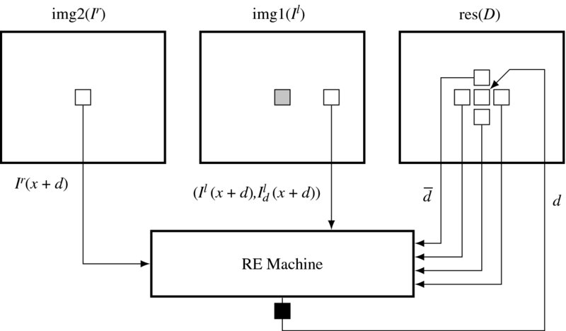
Figure 11.1 The flow of computation in the RE machine. Right reference mode. The shaded square is the current position. The RE machine is terminated by a pipelining register
For legibility reasons, only the circuit for the right reference system is shown. For the left reference system, the role of the images must be switched. The top three elements are the memories (Ir, Il) for the images, and D for the disparity map. They are the inputs and state memories of the RE machine. The other constructs are the sequential and combinational circuits, where the actual operations are executed. At a certain time, the memories are all fixed and the values in the combination circuits are actively being decided. Blocking the output port of the RE machine and connecting the combinational paths between the state memory and the blocking registers result in the system becoming a finite state machine (specifically, a Mealy machine), as a whole.
Within a given period, all the computation is done for Ir(x, y) in the right image plane (in right reference mode). The conjugate point Il(x + d(x, y)) is determined by reading the disparity at this pixel from the disparity map, D. The conjugate pairs and the neighborhoods around d(x, y) are used to determine the new disparity d(x, y), which is overwritten to the disparity map, D. In the next period, the same computation is executed for the next pixel. This computation is repeated for the frame until the disparity values converge. (Actually, in a simple design, the number of iterations is predetermined.)
11.5 Overall System
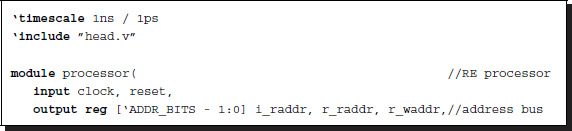
Keeping Figure 11.1 in mind, let us begin to design the Verilog HDL code. The header contains the parameters that characterize the images and the RE algorithm.
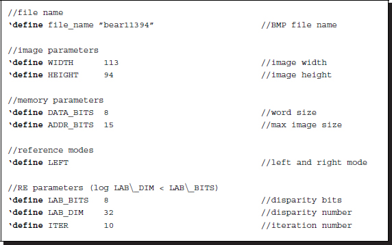
Listing 11.1 The header: head.v (1/9)
The filename is used for the IO part of the simulator to open and read the image files in the RAM, imitating the camera output. The image size, defined by the height and the width, M × N, is used in the specifying of the required resources throughout the circuit. The memory parameters specify the word length and the address range for the contents in the RAM. The image data is ordinarily stored in bytes – three bytes for RGB channels. These parameters are also used to define the arrays, img1, img2, and res, storing two images and a disparity map.
The next parameter is the key, LEFT, indicating the left or right reference mode. The window and the scan directions differ according to this parameter. The computation order is simply the raster scan direction in the right mode and the opposite of the raster scan direction in the left mode.
The RE parameters specify the word length of the disparity and also its maximum number. For a number of bits, B, the maximum disparity level, D, must be D ≤ 2B. Finally, the number of iterations is specified by ITER.
The template for the main part of the code is as follows.
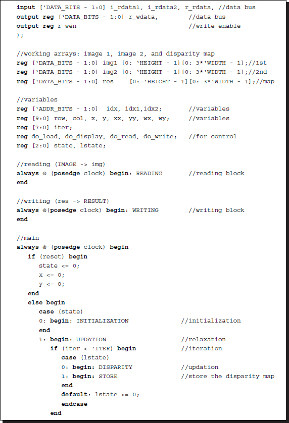
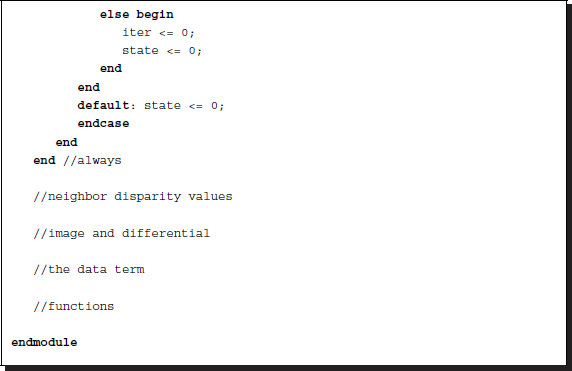
Listing 11.2 The framework: processor.v (2/9)
The code has three parts: sequential circuits, combinational circuits, and functions. The sequential part consists of three concurrent parts: reading, writing, and updation. The reading and writing blocks are the IP interfaces to the external RAMs, RAM1, RAM2, and RES, and the internal buffers, img1, img2, and res. The updation block writes the updated disparity to the disparity map. In this code, the disparity map is encoded as an unpacked array, res. However, the data vectors, data, are all coded in packed format for computational simplicity. While the sequential part works for each clock tick, the combinational part works between the clock period, reading the data from the registers and stabilizing the result, so that in the next clock tick the result can be stored in the registers. The combinational circuits have three parts: a circuit that builds the conjugate pairs, one that builds the data term, and another that determines the final disparity. The combinational circuits are aided by various functions, which all operate in the same simulation time.
The complexity of the code is as a result of the boundary conditions and the two modes. The related variables are the neighbor disparities, d0, d1, d2, d3, and the image values, Ir, Il, dI. The boundaries used in this code are mirror images. Other definitions are also possible (see the problems at the end of this chapter).
The components filling this template are explained in the ensuing sections.
11.6 IO Circuit
Two of the sequential circuits are for reading and writing. The image data are located in the external RAMs, outside of the main processor, and must be accessed periodically. The circuit can be designed as follows:
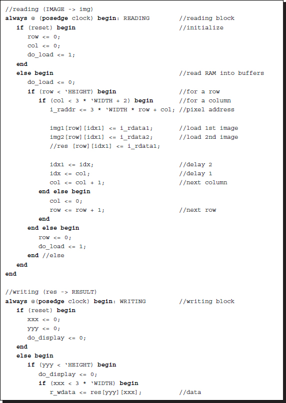
Listing 11.3 The IO circuit (3/9)
The purpose of the reading part is to read RAM1, RAM2, and RES into the internal buffers, img1, img2, and res. The processor reads the images (Il, Ir) and the disparity D from the buffers, processes them to determine the updated disparity, and writes the result into res. To match the address with the data, some small delays must be introduced into the address bus because a mismatch exists between the incoming data and the current address: the current data corresponds to the address two clocks ahead. These problems can be solved by the delay buffers idx and idx1 and the two clock delays in the address loop.
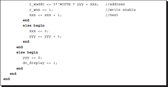
Another concurrent always block is the writing block. The purpose of this block is to write the disparity map stored in the buffer, res, into the external RAM, RESULT, in RGB format so that the simulator can display the disparity map in BMP format. The flags do_load and do_display are used to control the simulator and thus are not part of the synthesis. Note that the counters representing pixel positions, (row, col), (x, y), (xx, yy), and (xxx, yyy) are all differently redefined in different always blocks, to avoid driving a net variable with multiple drivers.
For simplicity, the IO circuit can be bypassed for simulation purposes by the unsynthesizable codes in io.v (see the problems in Chapter 4).
The remaining circuit can be considered a system that receives img1, img2, and res as inputs and returns an updated res as output.
11.7 Updation Circuit
The computation is based on window processing. There must be a circuit that relocates the window around the image plane. The constraint is that as a consequence of window movement, the entire image plane must be completely scanned, without producing empty spaces. In actuality, the space to be scanned is (x, y, l), where ![]() and l ∈ [0, L − 1] for some maximum iteration L. There is an algorithm called FBP (Jeong and Park 2004; Park and Jeong 2008) that can scan in the iteration index. For hierarchical BP (Yang et al. 2006), sampling in this space must be made in the pyramid form. The order of visits may be deterministic or random. In this chapter, we follow the usual approach: scanning the image plane in raster scan manner.
and l ∈ [0, L − 1] for some maximum iteration L. There is an algorithm called FBP (Jeong and Park 2004; Park and Jeong 2008) that can scan in the iteration index. For hierarchical BP (Yang et al. 2006), sampling in this space must be made in the pyramid form. The order of visits may be deterministic or random. In this chapter, we follow the usual approach: scanning the image plane in raster scan manner.
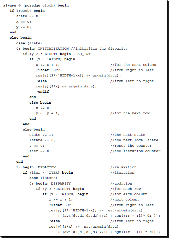
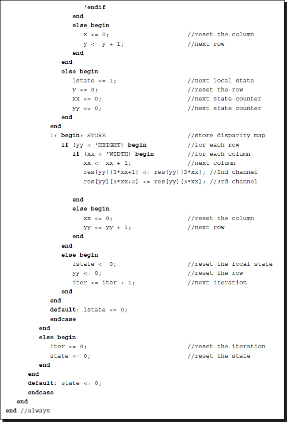
Listing 11.4 The updation circuit (4/9)
In iteration notation, the circuit spans the M × N × L × m × n space in (l, y, x) manner, where x is changed most rapidly and l is changed most slowly. Other iteration methods are also possible. For the right mode, the circuit scans from left to right, while for the left mode, it scans from right to left. The absolute positions of the pixels are (Ir(y, x), Il(y, x + d(x, y))) for the right mode and ![]() for the left mode.
for the left mode.
In the updation block, the new disparity is determined by the combination of three terms: data, neighborhood, and differential. The data term functions as a forcing term, preventing the solution from deviating too much from this value. To balance the dynamic range, the neighborhood average is reduced by half. Next in line is the differential, which guides the solution in the direction it must move. This differential is determined by the difference of the conjugate pairs and the slope of the matching image. The dynamic range of the disparity is very small, and so a large differential may result in an overflow or an underflow. To prevent such cases, we may take only the unit direction of the differential vector. Addition of the three terms again must be protected by the saturation function, which limits the number within the maximum disparity.
11.8 Circuit for the Data Term
From here onwards, all the computations are realized with combinational circuits, unless otherwise stated. The data vector, d(n), in Equation (11.9), is the major source of the belief message, driven by the input images, and thus must be provided accurately.
The circuit that provides this vector is depicted in Figure 11.2. As shown in the figure, the sources of the data vector are the two image frames. The location of the current pixel is indicated by a position in a frame. A specific field, d, of the data vector is constructed by the data read from the two images. Therefore, a data vector can be constructed concurrently for all the pixels of the two images on the same epipolar line. All the elements of the vector are determined by the combinational circuits, as follows.
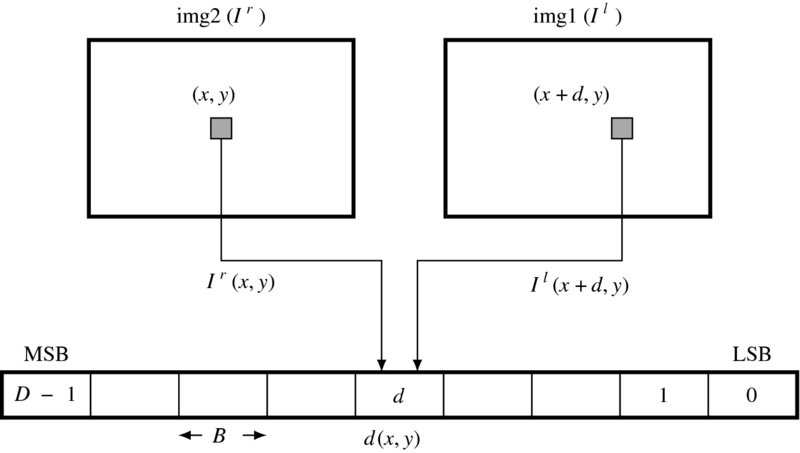
Figure 11.2 Building the data vector, d(x, y). The vector is generated by the combinational circuits for all elements in parallel (right reference mode)
The data vector is encoded in a packed array of BD bits, because it must be often accessed as one complete set of data. In the right reference system, the data term is
where dD − 1 is the MSB and d0 is the LSB. Each element is a B bit number with
Here, the data value is limited within B bit word length, preventing overflow.
For the left reference system, the data is defined as
Advanced algorithms may use different schemes to compute the data term, for example with better distance measure and perhaps an occlusion indicator. This code is the basic template and contains only the most basic features.
Keeping in mind the concept, we can code the algorithm as follows. Because there are numerous identical circuits, the Verilog generate construct is used. The code also contains the Verilog compiler directive to switch the design between the two reference modes.

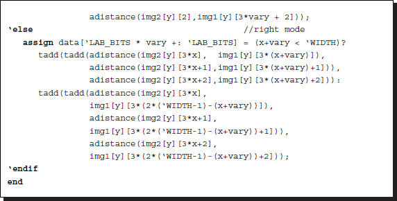
Listing 11.5 The data term: processor.v (5/9)
The circuits are compiled separately according to the two types of reference systems. Each reference system consists of D continuous assignments, with each assignment determining a B bit field in the data vector. The circuits are generated by the Verilog HDL generate construct. Consequently, this part of the circuit consists of D combinational circuits.
Two functions are used in the expression: adistance and tadd. The adistance function is an absolute function that returns the absolute distance between two arguments. The tadd function is an addition function that accounts for saturation math. The upper bound of the truncation is defined by 2B − 1. The functions, together with other functions, will be discussed together in a later section. The deciding minimum argument may be enhanced by introducing weights such as the truncated linear or Potts model.
The code is somewhat lengthy because of the boundary conditions. The mirror image is used around the boundary.
11.9 Circuit for the Differential
The next term related to the image inputs is the differential term. When the mirror image is adopted in the boundary values, the code becomes as follows.
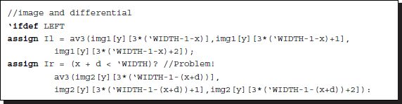
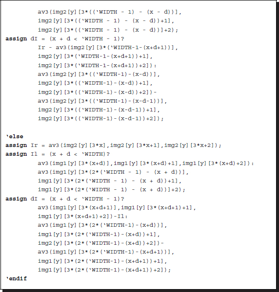
Listing 11.6 The data term: processor.v (6/9)
For the right mode, the corresponding pixel on the left image is offset by d, and thus may be located outside of the image frame. The conditionals check this condition and add mirrored values for such pixels. For the differential, the description is much more complicated because both terms are offset by d and d + 1, which may deviate from the image boundary. A similar situation occurs for the left mode system, but in opposite coordinates.
11.10 Circuit for the Neighborhood
The input disparity vector must be constructed in parallel with the data vector because they will be combined immediately afterwards. The circuit consists of only five continuous assignments.

Listing 11.7 The neighborhood: processor.v (7/9)
The circuit must also account for the boundary conditions. (Mirror image is used here.)
Note that the code is separated with the Verilog compiler directive for the right and left reference modes. The difference between the two modes is in their use of the counters to compute the coordinates. For the right mode, the conjugate point is on the right, while for the left mode, the conjugate point is on the left.
11.11 Functions for Saturation Arithmetic
The combinational circuits are aided by many functions. They provide a compact method to write the common codes in the function and task (although task is not used here). The restriction is that the codes must be executed within the same simulation time and the variables are all local. Because of the variable scopes, accessing the entire image or message matrix is very inefficient. Let us design the circuits for such functions.
The first function is tadd, which adds numbers and limits the size of the output to predefined bounds. Usually, the lower bound is zero and the upper bound is the full field, 2B − 1, where B is the word length of the message. This operation must be secured so that underflow and overflow are averted. All other functions doing any kind of addition may use this saturation math.
The second function is av, which takes two arguments and outputs their average value. To avoid any possible overflow, the arguments are halved before addition. All the arguments must be within the number range. The functions av3 and av4 are the expansions from two to three or four arguments. The function computes the average of the multiple arguments, calling av as required.
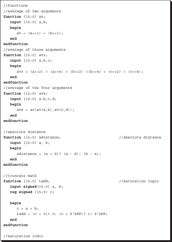

Listing 11.8 The functions (8/9)
In computing averages, shift operations are used to avoid division. However, a problem arises when finding the average of the three arguments because getting the exact average of the three arguments is not possible with shift operations. In general, for n arguments, we have to determine the coefficients ak, which is ak ∈ { − 1, 0, 1}:
where B is the word length of the arguments. For the three arguments, one of the best approximations is ![]() (see the problems at the end of this chapter).
(see the problems at the end of this chapter).
In addition to the additions, difference operations are needed to measure the likelihood of two numbers. The basic distance between two numbers is defined by the absolute distance, although other advanced distance measures can replace this. The function, adistance, serves this purpose in an integer word length.
11.12 Functions for Minimum Argument
At the end of the iteration, the messages are supposed to be in equilibrium. At this point, the final message is determined and therefore so is the disparity. This is the concept underlying the original theory. In actuality, the circuit executing this task is separated from the circuit utilized for the message updation and thus operates concurrently with the other circuits. Therefore, there is no reason to halt this circuit during the iteration.
In Equation (11.16), the required operation is
The function, argmin, returns the minimum argument, given the input vector.
This operation reads as follows in Verilog HDL.
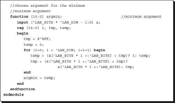
Listing 11.9 The functions (9/9)
It is important that a minimum near the center position be chosen when multiple minima exist throughout the elements in a vector. This is because the required value is not the message but its index, which must be as close to the current position as possible. The heavy weight must be designed so that this condition is guaranteed. Otherwise, the circuit will have to be redesigned in a more complicated manner.
11.13 Simulation
Thus far, we have derived the RE circuit. In order to successfully implement the design, it must first be optimized by removing as many of the warning signs as possible. If the design is correct, the synthesis parts, processor.v, pe.v, RAM1, RAM2, RES, excluding io.v, will all pass the synthesis stage. For the simulation, we used a pair of 225 × 188 images (CMU 2013; Middlebury 2013). The test images are depicted at the top of Figure 11.3. The lower images are the disparity maps, that is left and right reference modes.
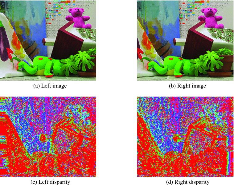
Figure 11.3 Disparity maps (image size: 225 × 188, disparity level: 32, iteration: 10, mirror-reflected boundary)
The parameters for the RE were as follows. The entire image frame was processed in a raster scan manner and the total number of iterations was 10.
The right reference map has a poor region on the right end. Likewise, the left reference map has a poor region on the left side (see the problems at the end of this chapter). The result is poorer than the disparity map obtained by the DP and BP machines. However, more weight for the neighborhood and preprocessing with smooth filtering may help to improve the performance.
In complexity view, the RE machine needs 3MNB bits to store the images and MNDB bits to store the disparity map, where B is the word length of the disparity and the image pixel, and D is the number of disparity levels. In later chapters, we will encounter the DP and BP machines. The RE machine is simple and fast. It is the starting point for all other vision processing circuits. Improvements can be made to it by modifying the relaxation equation with more sophisticated terms.
Problems
- 11.1 [Discretization] Derive the discretization of the second differential, ∂fxxf and ∂fbxxf.
- 11.2 [Discretization] Derive the third difference, ∂fffxxx and ∂fbfxxx. Discuss its properties. The higher-order derivatives can be interpreted as the Sobel operator (Bradski and Kaehler 2008; OpenCV 2013; Wikipedia 2013c), which can be obtained by convolving templates of lower order.
- 11.3 [Discretization] Derive Equation (11.10).
- 11.4 [Overall system] In Listing 11.2, the computation is based on the Gauss–Seidel method. How can you convert the circuit into the Jacobi method?
- 11.5 [Overall system] In Listing 11.2, the pixel value beyond the boundary is set by the mirror image. Instead of the mirror image, fix the values to zero.
- 11.6 [Overall system] In Listing 11.2, the pixel value beyond the boundary is set by the mirror image. Instead of the mirror image, fix the values to the boundary values.
- 11.7 [Overall system] Listing 11.2 is for the stereo matching. How can you implement the circuit for motion estimation?
- 11.8 [Saturation arithmetic] In Listing 11.8, function av3 is defined for the average of three arguments. The result should not exceed the maximum value and division must be avoided. Enhance the computation by introducing more terms.
- 11.9 [Simulation] In the right mode system, the disparity value becomes uncertain because the position is closer to the right boundary. The same is true for the left mode system on the left boundary. Derive the probability of the disparity located in the given region and discuss the uncertainty.
- 11.10 [Simulation] In the right mode system, the disparity value becomes uncertain because the position is closer to the right boundary. The same is true for the left mode system on the left boundary. Let the range of disparity be N′ ≤ N. Derive the probability and discuss the uncertainty.
References
- Aubert G and Kornprobst P 2006 Mathematical Problems in Image Processing: Partial Differential Equations and the Calculus of Variations (Applied Mathematical Sciences). Springer-Verlag.
- Bradski GR and Kaehler A 2008 Learning OpenCV. O'Reilly Media, Inc.
- CMU 2013 Cmu data set http://vasc.ri.cmu.edu/idb/html/stereo/ (accessed Sept. 4, 2013).
- Courant R and Hilbert D 1953 Methods of Mathematical Physics, vol. 1. Interscience Press.
- Fehrenbachy J and Mirebeauz J 2013 Small non-negative stencils for anisotropic diffusion http://arxiv.org/ pdf/1301.3925v1.pdf (accessed May 3, 2013).
- Horn BKP 1986 Robot Vision. MIT Press, Cambridge, Massachusetts.
- IEEE 2005 IEEE Standard for Verilog Hardware Description Language. IEEE.
- Ilyevsky A 2010 Digital Image Restoration by Multigrid Methods: Numerical Solution of Partial Differential Equations by Multigrid Methods for Removing Noise from Digital Pictures. Lambert Academic Publishing.
- Jeong H and Park S 2004 Generalized trellis stereo matching with systolic array Lecture Notes in Computer Science, vol. 3358, pp. 263–267.
- Middlebury U 2013 Middlebury stereo home page http://vision.middlebury.edu/stereo (accessed Sept. 4, 2013).
- OpenCV 2013 Sobel operator http://docs.opencv.org/modules/imgproc/doc/filtering.html (accessed Sept. 24, 2013).
- Park S and Jeong H 2008 Memory efficient iterative process on a two-dimensional first-order regular graph. Optics Letters 33, 74–76.
- Perona P and Malik J 1990Scale-space and edge detection using anisotropic diffusion. IEEE Trans. Pattern Anal. Mach. Intell. 12(7), 629–639.
- Scherzer O, Grasmair M, Grossauer H, Haltmeier M, and Lenzen F 2008 Variational Methods in Imaging Applied Mathematical Sciences. Springer-Verlag.
- Weickert J 2008 Anisotropic diffusion in image processing http://www.lpi.tel.uva.es/muitic/pim/docus/anisotropic_diffusion.pdf (accessed April 15, 2014).
- Wikipedia 2013a Euler–Lagrange equation http://en.wikipedia.org/wiki/Euler%E2%80%93Lagrange_equation (accessed May 3, 2013).
- Wikipedia 2013b Multigrid methods http://en.wikipedia.org/wiki/Multigrid_methods (accessed Sept. 23, 2013).
- Wikipedia 2013c Sobel operator http://en.wikipedia.org/wiki/Sobel_operator (accessed Sept. 24, 2013).
- Wikipedia 2013d Successive over-relaxation http://en.wikipedia.org/wiki/Successive_over-relaxation (accessed Sept. 24, 2013).
- Yang QX, Wang L, and Yang RG 2006 Real-time global stereo matching using hierarchical belief propagation BMVC, p. III:989.
- Young DM 1950 Iterative Methods for Solving Partial Difference Equations df Elliptical Type Phd thesis Harvard University.