
8
Relaxation for Energy Minimization
This chapter introduces the relaxation equation and architecture, one of the basic computing methods in energy minimization: relaxation, dynamic programming, message passing, graph cuts, and linear programming relaxation (LPR).
Early to intermediate vision has a common computation structure. One structure has the attributes to be computed defined on the pixels or a group of pixels. Another structure has the attribute in a pixel correlated with its neighbor values, as often modeled by MRF. Yet another structure has the attributes being obtainable by iteration, relaxing intermediate values, and reusing them for a better solution in a recursive way. We examine a computation structure that combines all these together in terms of representation and architecture.
First, we represent the relaxation equation in time and space in terms of its common structures – iteration, neighborhood computation, and concurrency – and thereby observe how the general computational architectures, Gauss–Seidel and Jacobi methods, can be combined and the numerous architectural variations that can be positioned between the two ends of the spectrum.
Next, we represent the relaxation in a graph, which is the product space of the image plane and iteration. The computation can be viewed in different ways, such as edge connections and spanning orders, in the graph. Deforming the graph in an affine manner, we obtain a new graph in which the connections enable different spanning orders. As a result of the graphical representations, we obtain three basic computational structures – the Gauss–Seidel–Jacob (GSJ) method, the diagonal method, and the vertical method. As regards computation order, the GSJ method completes the plane and advances to the next layer, but the diagonal and vertical methods operate in reverse. In terms of memory, the GSJ method requires RAM, whereas the diagonal and vertical methods require queues. Finally, we define hardware algorithms that are close to Verilog design, called RE and FRE machines, for the GSJ and vertical methods.
The later part of this chapter deals with the relaxation equation, an equation that is typical in computer vision. Starting from the energy equation, this chapter outlines how to derive the relaxation equation, following variational calculus, discretization, and iteration formation. Incidentally, isotropic and anisotropic diffusion are explained as common smoothness terms.
The RE and FRE machines and the relaxation equation form the bases of machine design in Chapter 11.
8.1 Euler–Lagrange Equation of the Energy Function
Relaxation labeling is a numerical method for solving the discrete labeling in Definition 5.1. In this approach, we are concerned with the decomposition of a complex computation into a network of simple local computations and the use of context in resolving ambiguities. As a result, the algorithm becomes parallel, with each process making use of the context to assist in labeling decisions. Relaxation operations were originally introduced to solve systems of linear equations. In relaxation labeling, the relaxation operations are extended, the solutions involve symbols rather than functions, and weights are attached to labels, which do not necessarily have a natural ordering.
Let us begin with the energy function in Definition 5.1:
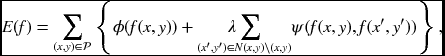
where λ is the Lagrange multiplier. The overall energy comprises a functional:
where F includes the data and prior terms:
The energy model may be enhanced by introducing a switch function multiplied to the second term, as in the case of occlusion modeling. The switch function can be modeled as a binary indicator or, more generally, as a differentiable function such as a sigmoid. Depending on the switch function, the ensuing derivation is rather different.
Minimizing the energy by using function f leads to the Euler–Lagrange equation (Courant and Hilbert 1953; Horn 1986; Wikipedia 2013b): The problem is the Euler–Lagrange equation with two functions and two variables:
In other cases in which the number of variables is greater than one, the number of Euler equations is also greater than one. To continue, we have to specify F( · ) further. The second term in Equation 8.1 signifies local variation, which is often modeled using differentials. Considering second-order derivatives, we get
This assumption is a simple example. There are many variations in which the smoothness term is models, which prelude the use of simple differentials. In most cases, problems occur when the range of variables is too wide to be approximated by Taylor series and/or the term is nonlinear because of some multiplied factors, such as occlusion terms. In addition, the measure can be other than the Euclidean metric, which makes the differential difficult. For such a case, the basic form of the relaxation equation is in fact often modified directly without undergoing the derivation process.
Substituting Equation (8.5) into Equation (8.4) yields
The Laplacian, ∇2, is related to the diffusion equation, ![]() , in thermal physics. The biharmonic operator (Polyanin and Zaitsev 2012), is related to the biharmonic equation ∇2∇2f = 0 in continuum mechanics.
, in thermal physics. The biharmonic operator (Polyanin and Zaitsev 2012), is related to the biharmonic equation ∇2∇2f = 0 in continuum mechanics.
The equations contain two major terms: Laplacian (Ursell 2007) and biharmonic operators (Polyanin and Zaitsev 2012):
The Euler equation for the general energy equation is compound because of the diffusion and biharmonic operators. In practical applications, only one of the two operators is adopted.
In its simplest form, the diffusion term is isotropic but in many cases, it becomes an anisotropic operator. Such cases arise when we deal with directive smoothing or determine local variations adaptively. For example, in edge preserving filtering, the smoothing must be differentiated from uniform and boundary regions. Anisotropic diffusion is made possible by introducing a nonlinear diffusion coefficient between the derivatives (Perona and Malik 1990):
Let us examine the properties of the Laplacian and biharmonic operators. The Euler–Lagrangian equation can be considered a filtering process of f, driven by the observed signal ϕf. The signal f is often smoothed by the Gaussian filter, allowing the linear filter to function as a Gaussian filter. The equation consists of two major terms: diffusion and biharmonic terms. The net result is the combination of the two filters and thus it is necessary to observe the homogeneous solution.
The Gaussian derivatives are conveniently represented by the Hermite polynomials (Wikipedia 2013d):
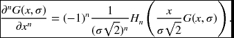
Then, up to fourth order, ∂nxG(x, σ)/G(x, σ) becomes
It is also well known that the Laplacian can be approximated by a DOG filter (Marr and Hildreth 1980). This property has been generalized to higher-order derivatives, with the proposal that the higher-order Gaussian filters can be constructed by linear summation of lower-order filters (De Ma and Li 1998; Ghosh et al. 2004).
The 2D Gaussian filter is represented by G(x, y, s, t), where s and t may be different for an anisotropic system:
Using the separability property and the Hermite series, we can derive higher-order 2D filters. In particular, the second order is
which is well-known as LoG and often approximated by DOG (Marr and Hildreth 1980). The biharmonic filter is the fourth-order Gaussian:
The filters are compared in Figure 8.1. The first row shows the Laplacian: ∇2G and ∇2G/G. The second row shows the biharmonic: ∇2 · ∇2G and ∇2 · ∇2G/G. The third row shows the composite filter: (∇2 + ∇2 · ∇2)G and (∇2 + ∇2 · ∇2)G/G.
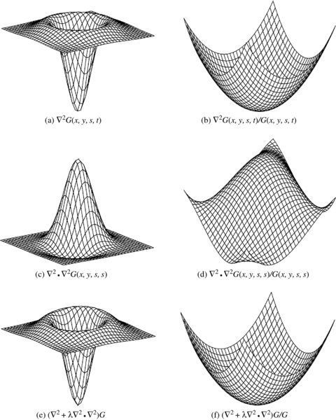
Figure 8.1 Shapes of Gaussian derivatives (s = 0.15, t = 0.15, and λ = 20)
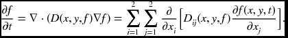
From another viewpoint, the diffusion operator in Equation (8.6) can be interpreted as a heat equation and thereby modeled in many different ways. The simple interpretation is the isotropic diffusion:
where D is a scalar called the diffusion coefficient. The solution of this equation is Gaussian (see the problems at the end of this chapter). The next level of the diffusion equation is anisotropic diffusion, in which the diffusion coefficient depends upon the coordinates:
where ‘∇ ·’ is the divergence operator. An even more general representation is the tensor diffusion, in which the scalar diffusion is extended to the diffusion tensor – a positive semi-definite symmetric matrix:
In image processing, the research on nonlinear diffusion is rooted in the following equation (Perona and Malik 1990):
where λ is a parameter. Such cases occur when we deal with directive smoothing or determine local variations adaptively. For example, in edge preserving filtering, the smoothing must be differentiated from the uniform region and the boundary region. Among the many, some examples are ∂f/∂t = ∇ · (|∇f|− 1∇f) (Rudin et al. 1992), ∂f/∂t = |∇f||k*∇f|∇ · (|∇f|− 1∇f) (Alvarez et al. 1992), and ![]() (Sochen et al. 1998). Presently, the diffusion equation has been extended significantly, up to the generalized heat equation:
(Sochen et al. 1998). Presently, the diffusion equation has been extended significantly, up to the generalized heat equation:
where F( · ) denotes a function (see (ter Haar Romeny 1994; Weickert 2008) for the surveys). If the problem is given by this heat equation, instead of the energy equation, the stage of obtaining the Euler equation is not needed. The relaxation equation is obtained directly by discretizing this equation:
For numerical computation, the terms on the right must be discretized accordingly.
Including anisotropic tensor and the biharmonic operator, the Euler–Lagrange equation becomes
In a simple but practical case, the Euler–Lagrange equation is often modeled by
Meaningful interpretation is possible if the data term satisfies certain conditions (Ursell 2007).
As a result, we have various levels of Euler–Lagrange equations: Equations (8.6), (8.19), and (8.20). The equations further depend on the diffusion model and the nonlinear term by g( · ).
8.2 Discrete Diffusion and Biharminic Operators
The Euler–Lagrange equations are completed only when the data term ϕf is known. Even so, it is very difficult to obtain an explicit solution. A practical approach is the numerical computation on the relaxation equations. To arrive at the relaxation equation, we need to discretize the Euler–Lagrange equation and then convert it into iterative form, while considering possible convergence. We then have to concentrate on the two terms: diffusion and biharmonic.
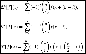
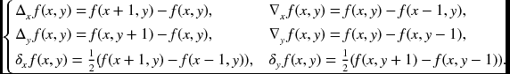
To begin with, we need to obtain kernels for the basic differentials. Let us represent the n-th-order differential ∂n/∂xn by the forward (Δn), and backward (∇n) and central (δn) difference operators (Wikipedia 2013c), which are
It is practical to use 3 × 3 templates for the differences in image processing. The templates for the second derivatives can be obtained by multiplying the first-order templates twice. In this case, the forward and backward templates are alternately multiplied to obtain efficient templates. In general, to make the higher-order difference kernel symmetric about a center point, the forward, backward, and central differences are mixed alternately. Some of the frequently used kernels are
Let us now return to Equation (8.6) to discretize the diffusion and biharmonic operators. The Laplacian operator can be approximated in many different ways (Wikipedia 2013a). The discrete Laplacian is often approximated by the five-point stencil:
The anisotropic diffusion operator in Equation (8.14) is approximated by
The derivation is all based on four neighbors and typical stencils among many.
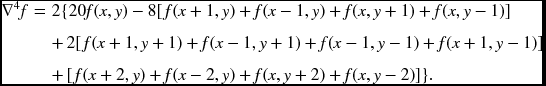
Similarly, the biharmonic operator can be discretized in many different ways (Chen et al. 2008). The standard stencil is the 13-point biharmonic operator that is obtained by applying the five-point diffusion operator twice.
There are a lot of issues surrounding modifying the kernel to compensate for errors on grid points near the boundary (Glowinski and Pironneau 1979).
8.3 SOR Equation
In the final stage, we have to convert the difference equation into SOR. The general concept of successive over relaxation (SOR) is as follows. If T( · ) is a contraction mapping,
then the corresponding SOR (Young 1950) can be obtained by
where ω is the relaxation parameter. The system is under-relaxation if ω < 1 and over-relaxation if 1 < ω < 2.
For Equation (8.20), we get the relaxation equation,
where ![]() denotes the four-neighbor average. The convergence speed can be adjusted by ω. Similarly, for Equation (8.6), we have
denotes the four-neighbor average. The convergence speed can be adjusted by ω. Similarly, for Equation (8.6), we have
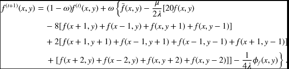
The parameters, λ, μ, and ω, play important roles in system stability. Actually, there is no unique way of deriving the SOR. Some may even lead to the system becoming unstable. The system can be more complicated if anisotropic diffusion and the enhanced biharmonic stencils are utilized. The complete expression is possible only when the data term ϕf is known. If ϕ = (T(f) − I)2, we get ϕf = 2(T(f) − I)Tf, which further reduces to ϕf = 2(f − I) if T(f) = f. If ϕ is known, the terms can be better modified, with the terms and relaxation parameter readjusted.
Equations (8.27) and (8.28) are typical in image processing, although the details may vary depending on the problems. If the data term is available, we can elaborate the equation by adding more terms and modifying the links between the terms by adding switching factors, which are otherwise difficult in the original energy function. In the next chapter, we derive this type of expression in stereo matching and thereby design appropriate relaxation machines.
8.4 Relaxation Equation
Thus far, we have derived a relaxation equation from a basic energy function. We will now expand the expression to a more general case. There are two types of relaxations in mathematical optimization: modeling strategy and iterative method. Relaxation as an iterative method solves a problem by generating a sequence of improved approximate solutions for the given problem until it reaches a termination condition, usually defined by convergent criteria. Relaxation as a modeling strategy solves a problem by converting the given difficult problem to an approximate one, relaxing the cost functions and constraints. The two methods are widely used in vision computation, as successive over-relaxation (SOR) for solving differential and nonlinear equations and as LPR for solving integer programming. In this chapter, we deal with the computational structure of iterative relaxation.
Relaxation is one of the most classical algorithms in computer vision that use iteration and neighborhood computation (Glazer 1984; Hinton 2007; Kittler and Illingworth 1985; Kittler et al. 1993; Terzopoulos 1986). This algorithm is a natural choice in solving many vision problems, because it is related with the operations: energy minimization, discretization, iterative computation, neighborhood computation.
In image processing, relaxation research is largely rooted in (Hummel and Zucker 1983). After a long evolution, relaxation has evolved up to message passing (Pearl 1982) and graph cut (Boykov et al. 1998). Beside the principles, there are also works on relaxation architectures pursuing parallelism (Gu and Wang 1992; Kamada et al. 1988; Mori et al. 1995; Wang et al. 1987) and hierarchical structures (Cohen and Cooper 1987; Hayes 1980; Miranker 1979).
From a computational point of view, relaxation algorithms can be characterized by the following factors: transformation, neighborhood topology, concurrent processing, initial and boundary conditions, computation order, and scale. The objective of the algorithm is to update the center pixel by concurrently mapping neighborhood values, following initialization, boundary condition, and computation order. Let us examine the factors individually below.
First, consider the transformation that maps the input state to a new state. For a point, ![]() , define a function f that maps the point to a vector,
, define a function f that maps the point to a vector, ![]() , where K means K-dimensional. In addition, define a function T that maps a neighborhood to its center node, T: N(p)↦p, where N(p) denotes the neighborhood of p, including itself. We can then define the relaxation equation by
, where K means K-dimensional. In addition, define a function T that maps a neighborhood to its center node, T: N(p)↦p, where N(p) denotes the neighborhood of p, including itself. We can then define the relaxation equation by
Here, t denotes time up to the maximum T. Usually, the iteration is continued until convergence but in practice it is terminated in a predefined time. The operation becomes a point-operation or neighborhood operation, depending on the neighborhood size. The mapping from neighbors to the center point is represented by a function and its parameters, which can be time-varying or time-invariant, fixed or variable connections, or linear or nonlinear.
For a linear time-invariant system, we get an IIR filter:
and for a linear time and shift invariant system, we get an FIR filter:
The operation can be as simple as the momentums: arithmetic mean, geometric mean, harmonic mean, contraharmonic mean, and the statistical momentum: median, max, min, midpoint, alpha-trimmed mean (Gonzalez et al. 2009), morphological operations, Nagao-Matsuyama filter (Nagao and Matsuyama 2013) and as complicated as message passing and graph cuts.
Relaxation is also characterized by neighborhood topology, which means a set of neighbor nodes and the connection to the center node. It may be variable or fixed in both time and space. Typical neighborhood systems are depicted in Figure 8.2. The three image planes, with different neighborhood connections, are shown at the top of the figure. The arrows signify influence between neighborhoods as opposed to physical connections. Below these images are the neighborhood definitions, consisting of a center pixel and neighbor pixels. In the three-neighborhood system, a node is connected to three neighbor nodes. Similarly, in four- and eight-neighborhood systems, a center pixel is connected to four or eight neighbors. Let us denote the neighborhood system by N3, N4, and N8. The three neighborhood systems are the simplest models of MRF, that is first-order Markov field. The rarest among them is the three-neighbor system such as summed area table (SAT) (Crow 1984) (see problems).
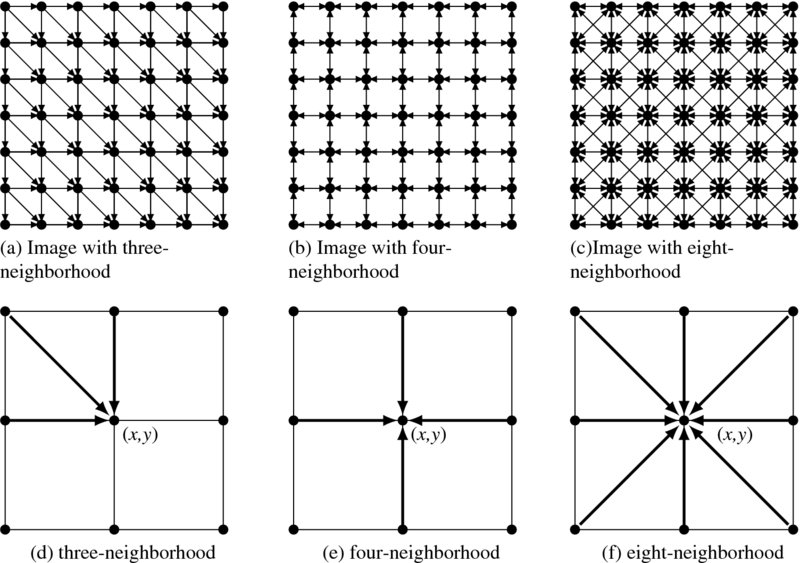
Figure 8.2 Neighborhood systems: (a)–(c) for images and (d)–(f) for neighborhoods
More specifically, the neighborhood systems are as follows:
In some cases, typically BP, it is convenient to represent neighbors relative to the center node: c(enter), e(ast), w(est), s(outh), n(orth), ne (north-east), se (south-east), sw (south-west), and nw (north-west), or using numbers clockwise from one to four: N4(p) = {p, e(p), w(p), s(p), n(p)} or N4 = {1, 2, 3, 4}.
Relaxation is also realized in parallel if possible. To achieve concurrent operations, we expand the center pixel to a window (or block) of pixels. The operation can then be executed window by window, with the nodes in the window all being maintained concurrently. Let A(p) denote a window around p and N(A(p)) the set of neighbors in A(p): N(A(p)) = {r|r ∈ N(q), q ∈ A(p)}. For such a window-based system, Equation (8.29) becomes
In short, let us call this RE (Relaxation Equation). This is a general representation for the features: neighborhood operation, iterative computation, and parallel processing.
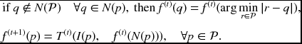
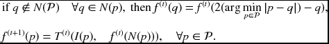
Relaxation algorithms are also characterized by initial and boundary conditions. For the initial condition, the initial value is normally ![]() . For the boundary condition, the neighbor may not be completely inside the image, provided that the center point is near the image boundary. For brevity, let
. For the boundary condition, the neighbor may not be completely inside the image, provided that the center point is near the image boundary. For brevity, let ![]() . There are two methods: global and local methods. In the global method, an additional step is needed for boundary management, along with the main computation. The border shrink method deals with those points whose neighbors are all in the image plane:
. There are two methods: global and local methods. In the global method, an additional step is needed for boundary management, along with the main computation. The border shrink method deals with those points whose neighbors are all in the image plane:
The result is a smaller area by the neighborhood size: ![]() . The zero padding method pads zeros in the exterior points.
. The zero padding method pads zeros in the exterior points.
The result is the same size as the image but it is influenced by the sudden changes of the image across the boundary. The other method is the border expansion method that pads the exterior using the nearby boundary values.
The boundary effect is less severe than the zero padding. The mirror expansion method fills the exterior points using the mirror image at the image boundary.
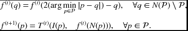
The result is less sensitive to local variations at the image boundary than other methods.
In the local method, the boundary is treated in each node locally on the fly. During the computation, each processor checks itself to determine whether it needs exterior values; if the answer is yes, it generates the exterior value, otherwise it continues. In this local method, additional logic is needed by the processors to check its position and generate the exterior values. For the border shrink method, each node executes the following:
The zero padding method is realized by the conditional execution:
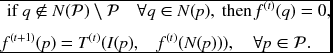
The border expansion method executes the relaxation in the following way:
Finally, the mirror expansion method executes locally:
The two methods have clear advantages and disadvantages. The local method is generally better for hardware design, for accessing exterior points with additional indexes, and for managing large memory with expanded boundaries, which are generally disadvantages in circuit design.
Relaxation algorithms are characterized by their order of computation. Let the image plane be ![]() and the iteration
and the iteration ![]() . A relaxation can be viewed as a process of visiting all the nodes in
. A relaxation can be viewed as a process of visiting all the nodes in ![]() in some proper order. For brevity, let (a(b(c))|A) represent a loop operation, where c changes most rapidly, a changes the slowest, and A represents block (window) processing.
in some proper order. For brevity, let (a(b(c))|A) represent a loop operation, where c changes most rapidly, a changes the slowest, and A represents block (window) processing.
The orders, (1(x(y))) or (1(y(x))), are one-pass algorithms, which are most desirable, at least for the elapsed time. This class of algorithms includes one-pass labeling and SUM. Represented by (2(x(y))) or (2(y(x))), two-pass algorithms determine the solution using two passes. In general, (t(x(y))) denotes a multi-pass algorithm, such as labeling, segmentation, morphology, filtering, connected-component, relaxation, BP, and GC, to name a few.
One of the most important multi-pass algorithms is the Gauss–Seidel method:
The proceeding order is the most usual scan, that is a raster scan. The neighbors are the most recently used (MRU) nodes. In contrast to raster scan, (t(x, y)) means that an entire image plane is updated concurrently, as in the Jacobi method.
Equation (8.33) includes Gauss–Seidel and Jacobi methods (Golub and Van Loan 1996; Press et al. 2007) as special cases. If the window size is a pixel, it reduces to Gauss–Seidel and if ![]() , it becomes the Jacobi method. The two methods are on opposite ends of the relaxation algorithms spectrum. In summary, a complete expression of relaxation must be constructed using Equation (8.33), mapping, concurrent processing, initial and boundary policy, neighborhood definition, and updation order.
, it becomes the Jacobi method. The two methods are on opposite ends of the relaxation algorithms spectrum. In summary, a complete expression of relaxation must be constructed using Equation (8.33), mapping, concurrent processing, initial and boundary policy, neighborhood definition, and updation order.
A very different scheme is possible using (x(y(t))) or (y(x(t))), which means that the computation proceeds in iteration axis first, then in the column (row) direction, and then the row (column) direction. To deal with all these methods in a coherent way, we first consider an efficient method for representing the computational space in the following section.
Finally, vision problems often involve multi-scale (or multi-resolution) problems. One of the approaches to the scale is using pyramidal hierarchy, in which the bottom and top levels indicate fine and coarse scales. This computational hierarchy is efficiently realized using the multigrid method (Heath 2002; Terzopoulos 1986; Wesseling 1992), which primarily performs smoothing, down-sampling, and interpolation. Pyramid algorithms are widely used in image representation and processing (Burt 1984; Jolion and Rosenfeld 1994; Kim et al. 2013; Lindeberg 1993).
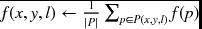
Suppose that a pyramid has levels l ∈ [ − L, U], where L and U are nonnegative integers representing, respectively, subpixel and coarse scales (Figure 8.3). The connection of the pyramid is the parent node P at the upper level and the children nodes C in the lower level. There are two types of pyramids: nonoverlapping and overlapping. For nonoverlapping pyramids, we define the nodes and connections such that for l ∈ [ − L, U], ![]() , S(x, y, l) = {(2x, 2y), (2x + 1, 2y), (2x, 2y + 1), (2x + 1, 2y + 1)}, and P(x, y, l) = {(⌊x/2⌋, ⌊y/2⌋)}. For overlapping pyramids, we define the nodes and connections such that for l ∈ [ − L, U],
, S(x, y, l) = {(2x, 2y), (2x + 1, 2y), (2x, 2y + 1), (2x + 1, 2y + 1)}, and P(x, y, l) = {(⌊x/2⌋, ⌊y/2⌋)}. For overlapping pyramids, we define the nodes and connections such that for l ∈ [ − L, U], ![]() , the candidate children are S(x, y, l) = {(2x + i, 2y + j)|i, j ∈ { − 1, 0, 1, 2}}, and the parents are P(x, y, l) = {(x + i)/2, (y + j)/2|i, j ∈ { − 1, 1}}.
, the candidate children are S(x, y, l) = {(2x + i, 2y + j)|i, j ∈ { − 1, 0, 1, 2}}, and the parents are P(x, y, l) = {(x + i)/2, (y + j)/2|i, j ∈ { − 1, 1}}.
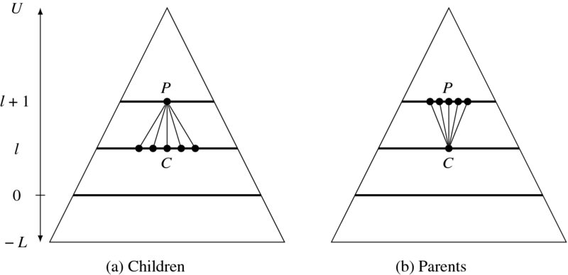
Figure 8.3 Pyramid hierarchy: (a) children and (b) parent
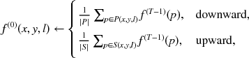
As inputs to the pyramid, the images are usually provided in image pyramid filtered using kernels such as Gaussian, Laplacian, and binomial coefficients. In a Gaussian pyramid, the image in each level Il is built by smoothing the adjacent level image with Gaussian kernel G(x, y) and down-sampling (↓) or up-sampling (↑):
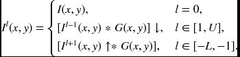
The control flow of the pyramid is also described by the upward and downward streams. In both directions, node operations are the same but the initialization is different. Depending on the directions, the node must be initialized by the average of the parent or the children.
where |P| and |S| are, respectively, the sizes of the parent and child.
In accordance with the conventions, the relaxation equation becomes
For a full description of relaxation, we have to specify all the factors as explained in an algorithmic form. Since the upward and downward control depends on application, we may have to write the downward algorithm only.
Algorithm 8.1 (Relaxation) Given I, compute the following.
- Input: image pyramid {Il|l ∈ [ − L, U]}.
- Output:
 .
. - Window: A(x, y) = {(x + i, y + j)|i ∈ [0, n − 1], j ∈ [0, m − 1]}.
- Boundary: global or local methods.
- for l = U, U − 1, …, −L,
- for t = 0, 1, …, T − 1 and
 ,
,
- if l = U and t = 0, f(x, y, l) ← 0,
- else if t = 0,
 ,
, - else f(A(x, y, l)) ← T(Il(A(x, y, l)), f(N(A(x, y, l)))).
We have now arrived at the final expression that includes all the major factors of relaxation: transformation, neighborhood, window, initialization, boundary condition, and scale. Even if the hierarchy has been considered, the major operation is the iterative updation, which is the same regardless of the level. Therefore, in the following section, we concentrate on the operation in a fixed level, as described by Equation (8.33) instead of Equation (8.46), unless otherwise stated.
8.5 Relaxation Graph
Computing RE can be viewed as determining all the nodes ![]() in systematic order. The space of the nodes can be considered as a stack of
in systematic order. The space of the nodes can be considered as a stack of ![]() planes numbered upwards with
planes numbered upwards with ![]() .
.
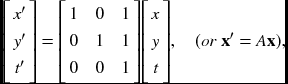
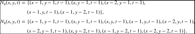
The concept is illustrated in Figure 8.4. The bottom layer represents an image plane while the top layer represents a result plane. In the side views, the vertical and diagonal edges represent the neighborhood connections from lower level to higher level. In the top view, the edges look like an ordinary four-neighborhood but they mean connections between successive layers. In this graph, we can view the RE as a method by which we determine nodes, one by one or window by window, from one layer to another layer in the upward direction. The top layer signifies the end of the iteration, and contains the final result.
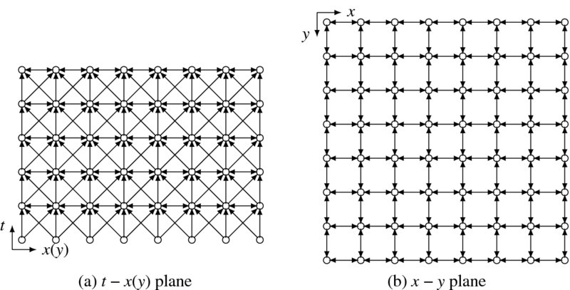
Figure 8.4 A graph G = (V, E, F) for relaxation (N4 system is shown)
This concept is formally defined as a graph G = (V, E, F).
Definition 8.1 (Relaxation graph) A relaxation graph G = (V, E, F) is a graph consisting of the nodes ![]() and the edges are defined in the neighborhood N(x, y, t) and connected bidirectionally in the same layer and unidirectionally from lower to upper layer. A node v ∈ V is assigned with a value
and the edges are defined in the neighborhood N(x, y, t) and connected bidirectionally in the same layer and unidirectionally from lower to upper layer. A node v ∈ V is assigned with a value ![]() . Especially, at the bottom plane,
. Especially, at the bottom plane, ![]() and at the top layer F(x, y, T − 1), the result is stored.
and at the top layer F(x, y, T − 1), the result is stored.
In the graph, the nodes on the bottom and top layers are special in that one is input and the other is output. Apart from this, all the other nodes are identical in their operation and connection.
Nodes on the same layer are connected bidirectionally, whereas nodes that are between two layers are connected unidirectionally. The connection is based on the neighborhood system: N3, N4, or N8. In this graph, the neighbor nodes are as follows:
Nodes in N4 and N8 are part of this node set.
In this graph, the computational order is not unique. For t, there is only one direction: increasing the order. However, x and y can proceed forward and backward. Consequently, there is a total of 24 possible methods. Gauss–Seidel and Jacobi are only two special cases, having the orders (t(y(x))) and (t(x, y)).
Among the many methods, only six are practical (Figure 8.5). The figure illustrates only the t − y section of V. It also shows the center node, neighbor connection, storage, and proceeding direction. This figure contains six basic orders of computation. Each row represents computing directions and each column represents neighborhood connections: Gauss–Seidel or Jacobi connections. Common to all the computing orders, the computation starts from the bottom layer, where the nodes are initialized by the input image and ends at the top layer, where the nodes contain the final result. In between, the nodes are updated, using the values in the neighbor nodes, which have already been visited and determined in the previous stage. The stored values and proper order facilitate recursive computation in the six cases. It is obvious that there are three different orders of computation: Gauss–Seidel–Jacobi, diagonal, and vertical methods. Let us examine the methods in more detail.
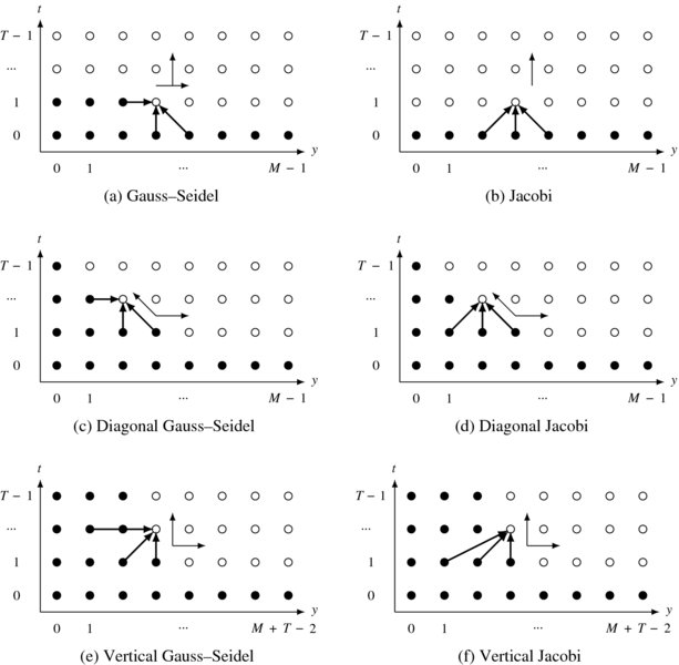
Figure 8.5 Basic methods of computation order
As the first figure shows, Gauss–Seidel, which has computation order (t(y(x))), is one possibility. The neighbor connection is defined by
where two neighbors are on the same layer and the other three are in the lower layer. The required storage is O(MN). The second method is Jacobi, which has computation order (t(x, y)). The neighbors are defined as
where all the neighbors belong to the lower layer. This method needs O(2MN) storage, for lower and upper layers.
Counterintuitively, the diagonal direction is possible for both Gauss–Seidel and Jacobi connections, as shown in the second row. The diagonal computation of the Gauss–Seidel connection is represented by (y − t(t(x))). The dual method (x − t(t(y))) is also possible. The required storage is O(NT). Similarly, the Jacobi connection can also be computed diagonally, with (y − t(t(x))) (or (x − t(t(y)))) order and O(NT) storage.
The shifted graph and connections are depicted on the third row. Instead of the original graph and diagonal direction, we may shift the graph so that the current node refers to those nodes whose index does not exceed that of the current node. In this manner, the diagonal computation can be converted to vertical direction for both Gauss–Seidel and Jacobi connections. The computation order is (y(x(t))) or (x(y(t))) and the storage is O(2NT).
The vertical computation is more than simplifying the diagonal computation. It actually contains three more variants: y, x, and x-y shifts. Shifting in the y-axis, as shown in the figure, results in vertical movement in the y-t plane. Likewise, shifting in the x-axis results in vertical movement in the x-t direction. There is a third transformation, in which the original graph is shifted in both the x and y directions. The result is diagonal movement in both the x-t and y-t planes. As a consequence, we will deal with the vertical structure, discarding the diagonal structures.
The two structures, GSJ and Non GSJ (nGSJ) for diagonal and vertical orders, show completely different properties in computation and are thus examined separately. In the following section, we examine the two structures in more detail and eventually represent them using hardware algorithms, called RE and FRE machines, intermediate representations between software algorithm and Verilog design.
8.6 Relaxation Machine
Let us first examine the GSJ structure. For the Gauss–Seidel method, the order is (t(y(x))) and the operation is
Among the five neighbors, two are new and three are old. Moving in the order, (t(y(x))), the operation is obviously recursive. Meanwhile, the Jacobi method has computation order O(t(x, y)) and operations,
All the neighbor values are located below the current plane. The operation is also recursive if the computation order (t(x, y)) is maintained.
For a closer look at the Gauss–Seidel method, three side views of G are illustrated in Figure 8.6. The views are the y-l, x-y, and a part of the x-y planes. The y-t view shows the connection between neighbors, located on the same layer and the lower layer. The shaded region is the minimal storage for recursive computation. The same computation is also observed in the x-y plane. The shaded region is the storage to be used later when the upper layer is updated. In the bottom is shown a window, A(x, y), an expanded version of a pixel, for window processing. Inside the window, the nodes located around the upper and left boundaries can access the most recently updated values while the others access older values in the lower layer. In fact, a window possesses both Gauss–Seidel and Jacobi properties. The boundary nodes belong to the Gauss–Seidel connection and the inner nodes belong to the Jacobi connection. As mn → 1, the system tends closer to the Gauss–Seidel method. Conversely, as mn → MN, the system tends closer to the Jacobi method. Between 1 < mn < MN, the system possesses properties of both the Gauss–Seidel and Jacobi methods.
Figure 8.6 Configurations: storage and connections for a node and window
In this manner, both the Gauss–Seidel and Jacobi methods are commonly represented by the window introduced. The RE becomes
which is a graphical representation of Equation (8.33). Here, N(A(x, y, t) is connected to the most recently updated nodes as explained: boundary nodes to the same layer and inner nodes to the lower layer.

If mn = 1, we have A(x, y, t) = {(x, y − 1, t), (x − 1, y, t), (x, y, t − 1), (x + 1, y, t − 1), (x, y + 1, t − 1)}. If mn = MN, we have A(x, y, t) = {(x, y − 1, t − 1), (x − 1, y, t − 1), (x, y, t − 1), (x + 1, y, t − 1), (x, y + 1, t − 1)}.
In addition to the updation equation, an algorithm needs more information about initial condition, boundary condition, control, and memory. It is summarized as follows:
Algorithm 8.2 (RE machine) Given I, determine f.
- Input:
 .
. - Memory:
 .
. - Window: A(x, y) = {(x + i, y + j)|i ∈ [0, n − 1], j ∈ [0, m − 1]}.
- Boundary: global or local method.
- Output:
 .
.
- Initialization:
 .
. - for t = 0, 1, …, T − 1,
- for y = 0, m, 2m, …, M − 1, for x = 0, n, 2n, …, N − 1,
- for y = 0, m, 2m, …, M − 1, for x = 0, n, 2n, …, N − 1,
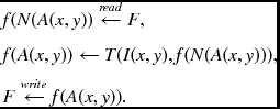
Let us call this the RE machine (relaxation equation machine). This machine needs two memories, a memory F and a window A, and a logic, global, or local boundary policy. In this algorithm, the detailed expression, represented by Equation (8.53), is not required, because the memory always contains the most recent values. Initially, the memory is simply overwritten with the image. The same operation is then repeated for all nodes in three nested loops. In each operation, a block of neighbors is read from the memory and used in the updation equation. The updated window is then overwritten on the older values in the memory. When the operation reaches the top and is finally over, the final result is the contents in the memory.
Considered in the computational complexity, the variables are the neighborhood N( · ) and the window size mn. This system requires O(mn) processors, O(MNT/mn) time, and O(MN + mn) space. At one extreme, it approaches the Gauss–Seidel method as mn → 1, which executes the algorithm with one processor, O(MNL) time, and O(MN) space. At the other end, as mn → MN, it approaches the Jacobi method, which uses O(MN) processors, O(T) time, and O(2MN) space. (Two memories are required in this case for input and output. The roles are alternatively changed in each iteration.) In general, the degree of serial and parallel computation is controlled by the parameter mn.
The corresponding architecture consists of a combinational circuit T( · ), a memory plane F, a buffer memory f(A), and three clocks (t(y(x))) (Figure 8.7). The clocks are represented by the three nested loops, (t(y(x))), with x for the innermost loop and t the outermost loop. There are no conditional jumps: the logic is completely deterministic. The image is stored in I and read in each clock period.
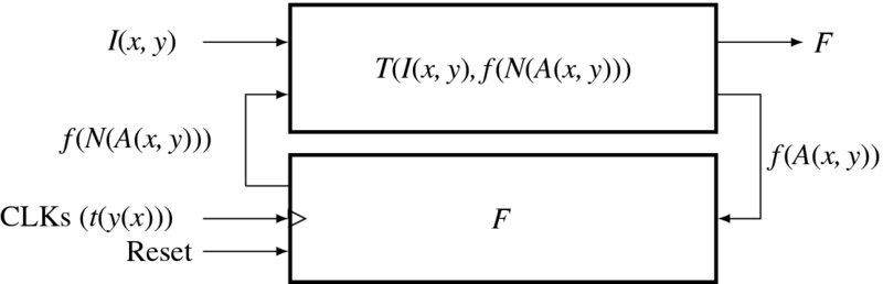
Figure 8.7 Architecture of the RE machine
8.7 Affine Graph
In Figure 8.5, we observed that the computational order can be (y − t(t(x))) or (x − t(t(y))). However, the diagonal direction is somewhat complicated when counting node numbers and preserving memories and thus more convenient representation is needed. There are three possibilities for shift directions: x, y, and x-y directions. Of the three, the third option is the best because it can use more updated neighbors than the others.
This concept is shown in Figure 8.8. If we push the graph in both the x and y directions, proportionally to the layer height – an affine transformation, the shape becomes a parallelepiped – the top plane is still parallel to the image plane but the other walls are no longer orthogonal to the image plane. Between two adjacent layers, the amount of shift is just one unit in both directions. Therefore, the neighborhood connection must also be shifted properly. For better understanding, three views are provided. The proceeding direction is the raster scan in both the l-y and x-y planes. In this order and connection, the neighbor values are always the most recently updated ones. This is one of many possible variations of deformation (see the problems at the end of this chapter).
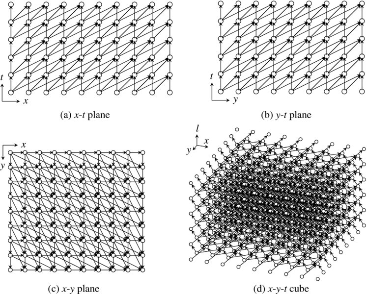
Figure 8.8 The induced graph, G′ = (V, E, F)
Because of the deformation, the original cube (rectangular parallelepiped) becomes a parallelepiped. To make the graph a rectangular parallelepiped, we fill the empty spaces with dummy nodes, which function the same way as the nodes. The resulting shape is a cube with N′ × T′ nodes, where N′ = (N + T − 1) and M′ = (M + T − 1). In this cube, the image input is still the M × N part of the bottom layer and the output is the same size as the top layer. Now, G′ can be considered G, except that the cube is expanded and the nodes are connected differently.
Let us define the induced graph formally and call it an affine graph.
Definition 8.2 (Affine graph) An affine graph G′ = (V, E, F) is a graph that is induced from the relaxation graph G by applying the affine transformation, which transforms (x, y, t) ∈ G to (x′, y′, t′) ∈ G′, using
where A is an affine matrix, and padding nodes so that the graph becomes a rectangular parallelepiped with ![]() , where N′ = N + T − 1 and M′ = M + T − 1.
, where N′ = N + T − 1 and M′ = M + T − 1.
The affine transformation can only be applied to one direction, in either x or y, but not both. In this case, we obtain different types of graphs in terms of neighborhood connections (see the problems at the end of this chapter). The two graphs differ in two aspects: first, the space is changed from M × N × T to M′ × N′ × T. Second, the original neighborhood must also be transformed by N′ = AN.
The neighborhood systems in Equation (8.32) become
In this expression, all the neighbors are positioned below and withdraw one or two cell distances from the center node.
The connections are illustrated in Figure 8.9. The filled dots are on the lower layer and the empty dots are on the upper layer. In the new graph, the neighborhood connections look distorted and thus the original bearings – east, west, south, and north – are not correct; however, we will keep the same name for simplicity. The node distances are also changed. The east and south neighbors are in one pixel distance but the west and north neighbors are in two pixels distance (in one coordinate).
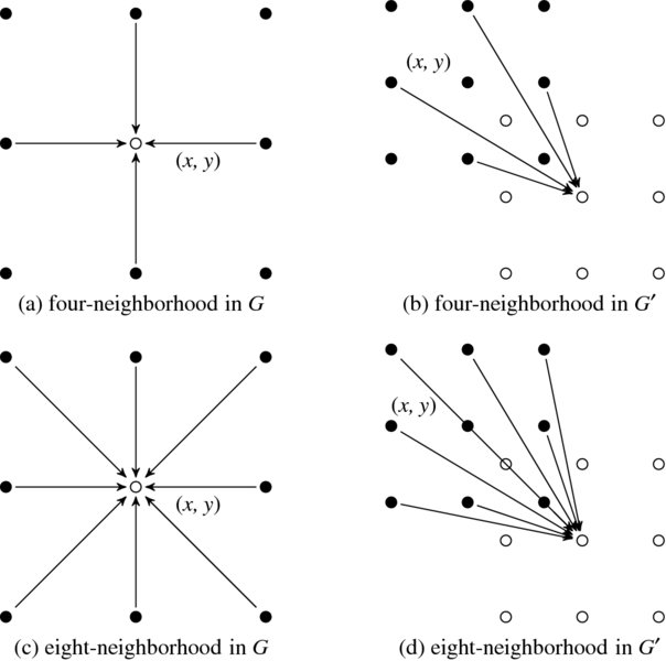
Figure 8.9 Neighborhood systems in G and G′. Empty circles are one level above the dark circles. The edge direction means data dependency
8.8 Fast Relaxation Machine
In G′, one of the efficient schedules is (y(x(t))), where the computation proceeds in the order, layer, column, and row. A node (x, y, t) can then be computed recursively using the previous values.

Here, I(x, y) is the new input while all the other values are stored values that were computed in the previous stages.
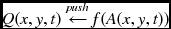
Let us expand the recursive computation from a node, (x, y, t), to a small window, A(x, y, t), whose position is represented by the first pixel position in it: A(x, y) = {(x + i, y + j)|i ∈ [0, n − 1], j ∈ [0, m − 1]}. The value set is f(A(x, y)) = {f(x + i, y + j)|i ∈ [0, n − 1], j ∈ [0, m − 1]}. The relaxation equation thus becomes
where y = 0, m, …, M′ − 1, x = 0, n, …, N′ − 1, and t = 0, 1, …, L − 1. Notice that starting from Equation (8.33), we have derived Equation (8.52) and Equation (8.57). The three equations represent the same RE but in different spaces – time, G, and G′. This method divides the x-y plane into m × n blocks and scans the plane block by block.
Together with the scheduling and hardware resources, this method is described as follows:
Algorithm 8.3 (fast relaxation machine) Given I, determine f.
- Input:
 .
. - Queue:
 .
. - Window: A(x, y) = {(x + k, y + t)|k ∈ [0, n − 1], l ∈ [0, m − 1]}.
- Boundary: global or local boundary policy.
- Output: f(A(x, y, T − 1)).
- Initialization:
 .
. - for y = 0, m, …, M′ − 1, for x = 0, n, …, N′ − 1, for t = 0, 1, …, L − 1, compute
 .
. .
. .
.- if t = T − 1, output f(A(x, y, T − 1)).
To differentiate this machine from the RE machine, let us call it the FRE Machine (fast relaxation equation machine). The major difference from the RE machine is the memory type: queue. The reading and writing positions, defined by f(N(A(x, y, t))), are fixed but the memory must shift down as the node position changes. Alternatively, the opposite is possible: fixed memory and moving address. The memory position is determined by the neighborhood type and the window shape. At the bottom layer, the processors do not need neighborhood but input image. At the first column, only one neighbor is available and thus others must be empty. Otherwise, the image input is not available and thus the processors use neighbor values only. The state memory must also be avoided at the top layer, since it will never be used. Whenever the processors move upward, the neighbor values must be read from the state memory. The output is available when the processors complete the top layer. This algorithm uses O(mn) processors and ((N′/n + 1)(L − 1))mn space. If mn → 1 and L → 2, it approaches the Jacobi machine but never approaches the Gauss–Seidel machine.
The architecture is shown in Figure 8.10. The system is driven by the three nested clocks, (y(x(t))), where the variables respectively denote the block number, row, column, and layer, with t the fastest and y the slowest. The addresses to the state memory blocks and pixels are all computed by the neighborhood relationship in a window. With image and neighbor values, the m × n processors compute the node values f(A(x, y, t)). After the updation, the state memory is written with this value when it is not on the top layer. This architecture is relatively easy to realize, because the memory structure is rather simple.
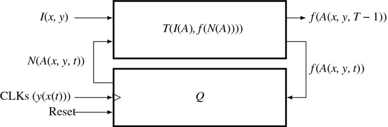
Figure 8.10 The block relaxation machine
For a complete system, the machines are the major part in Algorithm 8.1, which includes hierarchical control. However, those controls are largely dependent upon the problems and applications.
8.9 State Memory of Fast Relaxation Machine
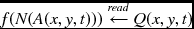
To completely describe FRE, we have to specify f(N(A(x, y, t))), by computing the positions of the neighbors in the memory. There are two possibilities for the memory: RAM and queue. For RAM, the addresses N(A(x, y, t)) are changed to write and read the memory and thus no further explanation is needed. For queue, the addresses are fixed and the contents are shifted down in the queue whenever the window moves to the next position. Unless otherwise stated, we assume a queue.
Let us consider a 2 × 2 window, A, in a graph G′ (Figure 8.11). The window moves according to the schedule, (y(x(t))). The left figure indicates a y-t plane view, which consists of an M′ × T grid, with bottom representing image plane and the top representing the result. In both views, the neighbor values are indicated by the connecting lines the state memory is denoted by the shaded region. In the y-t plane, the window moves in (y(t)) order. The state memory is a 4 × T rectangular in this plane. As the window moves upwards, the top of the memory is filled and the tail is emptied, so that the queue moves upwards. On reaching the top layer, the window shifts from y to y + 2.
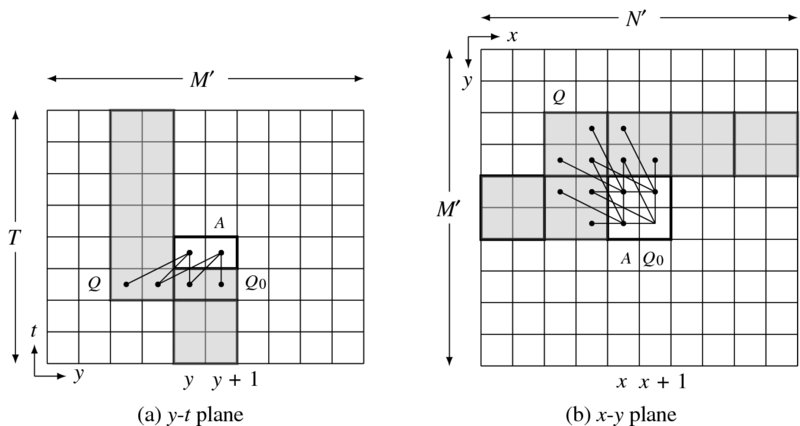
Figure 8.11 System state in y-t and x-y planes. A block (2 × 4), a state memory, and a buffer
In the x-y plane, the window moves in (y(x)) order. The node inside the window accesses the neighbor nodes as the links indicate. The memory in this view occupies the 2 × N′ rectangular region. From both views, the state memory becomes a 2 × T × N′ cube. The memory structure is primarily a queue, which can be conveniently realized with an array. To fully specify the neighborhood, we have to specify the addresses, relative to the present window. The addresses depend on the window position, (x, y, t) and the window size, (m, n).
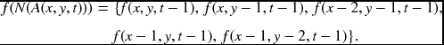
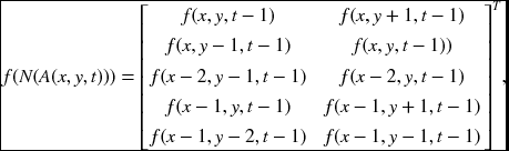
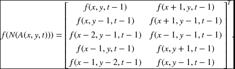
Typical examples are depicted in Figure 8.12. The figure contains four windows and the neighbor connections. Nodes in a window access other nodes as indicated by the lines. The shaded area is a part of the system memory that contains the neighbor values to be used presently and later. For simplicity, some unused memory cells are also included to make the memory structure more regular. The addresses indicated by the connecting lines clearly depend upon the window and image size.
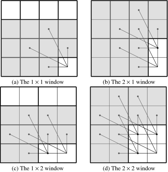
Figure 8.12 The windows and neighborhoods: 1 × 1, 2 × 1, 1 × 2, and 2 × 2
Let us first consider the 1 × 1 window, which is located at (x, y, t). If a queue is used, the memory is a rectangular parallelepiped with 3N′T nodes. The neighborhood pixels are located in five different places in the memory. When ordered in east, west, south, and north, the neighbor values are as follows:
The addresses represent the absolute positions in RAM. If a queue is to be used, the offset from (x, y, t) is the fixed address in memory. This concept is the same for other windows.
For a two-pixel window, we have two possibilities, specifically, 1 × 2 and 2 × 1 windows. There appears to be no preference about this but the 2 × 1 window seems to be somewhat simpler, because its height matches the state memory size. For the 2 × 1 window, two nodes independently access 10 cells in the memory, which has size 3N′T. The absolute positions are defined by
where the first row contains the neighbors of (x, y, t) and the second row the neighbors of (x, y + 1, t), all arranged in the order center, east, west, south, and north.
For the 1 × 2 window, the size of the memory is 2N′T. The memory addresses are
Likewise, in the 2 × 1 window, this window also accesses 10 neighbors, but in different positions. The first and the second rows, respectively, correspond to the neighbors of (x, y, t) and (x + 1, y, t).
The 2 × 2 window has 20 elements in the memory, which has 4N′T nodes. The neighborhood is defined by
where time indices are dropped for simplicity. The neighbors are ordered in a row, for (x, y, t), (x, y + 1, t), (x + 1, y, t), and (x + 1, y + 1, t), with the same four bearings.
In general, for an (m, n) window, the neighborhood values are determined by
The addresses denote absolute positions in RAM, which is organized in the shape of a ‘V’. If the memory is organized in other multidimensional arrays, the addresses must be converted accordingly. Moreover, if a queue is used instead, the addresses must be converted to the fixed positions in that memory.
8.10 Comparison of Relaxation Machines
Thus far, we have derived various architectures that possess some major properties of relaxation operations. We have defined a relaxation equation and, based on a graphical representation, obtained RE and FRE machines (Park and Jeong 2008a,b). The machines are all summarized in Table 8.1 and compared with time, space, and space-time product.
Table 8.1 Relaxation machines
| Machine | PEs | Time | Space | Space-Time Product | Memory |
| Gauss–Seidel | 1 | MNT | MN | M2N2T | RAM |
| Jacobi | MN | T | 2MN | 2MNT | RAM |
| RE (m × n) | mn | MNT/mn | MN + mn | MNT(MN + mn)/mn | RAM |
| FRE (1 × 1) | 1 | M′N′T | 3N′T | 3M′N′2T2 | Queue |
| FRE (2 × 1) | 2 | M′N′T/2 | 4N′T | 2M′N′2T2 | Queue |
| FRE (1 × 2) | 2 | M′N′T/2 | 3N′T | 3M′N′2T2/2 | Queue |
| FRE (2 × 2) | 4 | M′N′T/4 | 4N′T | M′N′2T2 | Queue |
| FRE (m × n) | mn | M′N′T/mn | (2 + m)N′T | (2 + m)M′N′2T2/mn | Queue |
cf. M′ = M + T − 1, N′ = N + T − 1, m ∈ [1, M], n ∈ [1, N].
The machines included in this table are classified into two classes: RE and FRE machines. The major difference between the two machines is the direction of computation, that is (t(y(x))) and (t(x, y)) or (y(x(t))). The RE machine is a unified concept of the Gauss–Seidel (mn = 1) and the Jacobi methods (mn = MN). The FRE machine is a rather different concept, whose extreme is also the Jacobi machine (mn = MN). Thus, the Jacobi method is the common connection between the two machines. The memories are all RAM, but queue is more natural to FRE. In RAM, the address moves and the content remains in the same position. In queue, the address is fixed and the contents are shifted. All the methods are scalable using the parameter mn, denoting the number of parallel processors. One of the advantages of the FRE over the RE machine is the far smaller memory.
Problems
- 8.1 [Euler–Lagrange Equation] Prove that the Gaussian distribution is the solution of the diffusion equation.
- 8.2 [Discretization] What stencils are possible, other than Equation (8.22), for ∇2f(x, y)?
- 8.3 [Discretization] Derive Equation (8.23), which is a discretization of anisotropic diffusion operator.
- 8.4 [SOR] For the above anisotropic diffusion, derive the relaxation equation for Equation (8.6), similarly to Equation (8.28).
- 8.5 [Relaxation equation] The relaxation technique originated from the iterative solution of linear systems. Let Ax = b, where
 and
and  . One of the approaches is to partition A into two matrices, A = N − M. Using this method, derive a relaxation equation and discuss the convergence conditions.
 - 8.6 [Relaxation equation] In deriving relaxation for Ax = b, we may partition A into three matrices. Using this method, derive the Jacobi method in matrix form.
- 8.7 [Relaxation equation] As a continuation of the previous problem, derive the Gauss–Seidel method in matrix form, using the three partitioned matrices.
- 8.8 [Relaxation equation] As a continuation of the previous problem, derive SOR in matrix form for the Gauss–Seidel method.
- 8.9 [Affine graph] In the affine graph, the transformation is applied in both directions, x and y. What happens to the neighborhood connection if the transformation is applied in only one direction?
- 8.10 [FRE machine] There is another type of algorithm that is different from the four-neighborhood processing, called sum area table (SAT). The SAT (also known as integral table) (Viola and Jones 2001) uses a three-neighborhood system and raster scan for computing area using just the previously stored values. It is a data structure and an algorithm for quickly and efficiently generating the sum of values in a rectangular subset of a grid. Write the updation equation for SAT and show that it is a one-pass algorithm.
- 8.11 [FRE machine] The original SAT algorithm means mainly fast summation, but inherently implies an efficient computational structure. In the SAT algorithm, show that the state memory can be realized with a queue, and rewrite the updation equation in terms of the queue.
- 8.12 [FRE machine] Derive the SAT in the above problem with corresponding algorithm and machine architecture, as we have done for the RE and FRE machines.
References
- Alvarez L, Lions PL, and Morel JM 1992 Image selective smoothing and edge detection by nonlinear diffusion. ii. SIAM Journal on Numerical Analysis 29(3), 845–866.
- Boykov Y, Veksler O, and Zabih R 1998 Markov random fields with efficient approximations. International Conference on Computer Vision and Pattern Recognition (CVPR).
- Burt PJ 1984 The Pyramid as a Structure for Efficient Computation. Springer.
- Chen G, Li Z, and Lin P 2008 A fast finite difference method for biharmonic equations on irregular domains and its application to an incompressible Stokes flow. Advances in Computational Mathematics 29(2), 113–133.
- Cohen FS and Cooper DB 1987 Simple parallel hierarchical and relaxation algorithms for segmenting noncausal Markovian random fields. IEEE Trans. Pattern Anal. Mach. Intell. 9(2), 195–219.
- Courant R and Hilbert D 1953 Methods of Mathematical Physics, vol. 1. Interscience Press.
- Crow FC 1984 Summed-area tables for texture mapping. Computer Graphics (SIGGRAPH '84 Proceedings), pp. 207–212. Published as Computer Graphics (SIGGRAPH '84 Proceedings), volume 18, number 3.
- De Ma S and Li B 1998 Derivative computation by multiscale filters. Image and Vision Computing 16(1), 43–53.
- Ghosh K, Sarkar S, and Bhaumik K 2004 A bio-inspired model for multi-scale representation of even order Gaussian derivatives. Intelligent Sensors, Sensor Networks and Information Processing Conference, 2004. Proceedings of the 2004, pp. 497–502 IEEE.
- Glazer F 1984 Multilevel Relaxation in Low-level Computer Vision. Springer.
- Glowinski R and Pironneau O 1979 Numerical methods for the first biharmonic equation and for the two-dimensional Stokes problem. SIAM Review 21(2), 167–212.
- Golub GH and Van Loan CF 1996 Matrix Computation John Hopkins Studies in the Mathematical Sciences third edn. Johns Hopkins University Press, Baltimore, Maryland.
- Gonzalez RC, Woods RE, and Eddins SL 2009 Digital image processing using MATLAB(R), 2nd edition Gatesmark Publishing.
- Gu J and Wang W 1992 A novel discrete relaxation architecture. IEEE Trans. Pattern Anal. Mach. Intell. 14(8), 857–865.
- Hayes KC 1980 Reading handwritten words using hierarchical relaxation. Computer Graphics and Image Processing 14(4), 344–364.
- Heath M 2002 Scientific Computing: an Introductory Survey. McGraw-Hill Higher Education. McGraw-Hill.
- Hinton GE 2007 Learning multiple layers of representation. Trends in Cognitive Science 11(10), 428–434.
- Horn BKP 1986 Robot Vision. MIT Press, Cambridge, Massachusetts.
- Hummel RA and Zucker SW 1983 On the foundations of relaxation labeling processes. IEEE Trans. Pattern Anal. Mach. Intell. 5(3), 267–287.
- Jolion JM and Rosenfeld A 1994 A Pyramid Framework for Early Vision: Multiresolutional Computer Vision. Kluwer Academic Publishers.
- Kamada M, Toraichi K, Mori R, Yamamoto K, and Yamada H 1988 A parallel architecture for relaxation operations. Pattern Recognition 21(2), 175–181.
- Kim J, Liu C, Sha F, and Grauman K 2013 Deformable spatial pyramid matching for fast dense correspondences. Computer Vision and Pattern Recognition (CVPR), 2013 IEEE Conference on, pp. 2307–2314 IEEE.
- Kittler J and Illingworth J 1985 Relaxation labelling algorithms: Review. Image and Vision Computing 3(4), 206–216.
- Kittler J, Christmas WJ, and Petrou M 1993 Probabilistic relaxation for matching problems in computer vision. Computer Vision, 1993. Proceedings, Fourth International Conference on, pp. 666–673 IEEE.
- Lindeberg T 1993 Scale-Space Theory in Computer Vision. Kluwer.
- Marr D and Hildreth E 1980 Theory of edge detection. Proceedings of the Royal Society of London. Series B. Biological Sciences 207(1167), 187–217.
- Miranker WL 1979 Hierarchical relaxation. Computing 23(3), 267–285.
- Mori K, Horiuchi T, Wada K, and Toraichi K 1995 A parallel relaxation architecture for handwritten character recognition. Communications, Computers, and Signal Processing, 1995. Proceedings, IEEE Pacific Rim Conference on, pp. 74–77 IEEE.
- Nagao and Matsuyama 2013 http://anorkey.com/nagao-matsuyama-filter/ (accessed May 3, 2013).
- Park S and Jeong H 2008a High-speed parallel very large scale integration architecture for global stereo matching. Journal of Electronic Imaging 17(1), 010501–3.
- Park S and Jeong H 2008b Memory efficient iterative process on a two-dimensional first-order regular graph. Optics Letters 33, 74–76.
- Pearl J 1982 Reverend Bayes on inference engines: A distributed hierarchical approach. In AAAI (ed. Waltz D), pp. 133–136. AAAI Press.
- Perona P and Malik J 1990 Scale-space and edge detection using anisotropic diffusion. IEEE Trans. Pattern Anal. Mach. Intell. 12(7), 629–639.
- Polyanin A and Zaitsev V 2012 Handbook of Nonlinear Partial Differential Equations second edn. CRC Press.
- Press WH, Teukolsky SA, Vetterling WT, and Flannery BP 2007 Numerical Recipes: The Art of Scientific Computing. Cambridge Univ. Press.
- Rudin LI, Osher S, and Fatemi E 1992 Nonlinear Total Variation based noise removal algorithms. Physica D: Nonlinear Phenomena 60(1), 259–268.
- Sochen N, Kimmel R, and Malladi R 1998 A general framework for low level vision. IEEE Trans. Image Processing 7(3), 310–318.
- ter Haar Romeny B 1994 Geometry-driven Diffusion in Computer Vision. Kluwer Academic Dordrecht.
- Terzopoulos D 1986 Image analysis using multigrid relaxation methods. IEEE Trans. Pattern Anal. Mach. Intell. 8(2), 129–139.
- Ursell TS 2007 The diffusion equation a multi-dimensional tutorial http://dl.dropbox.com/u/46147408/tutorials/diffusion.pdf (accessed Nov. 1, 2013).
- Viola P and Jones MJ 2001 Robust real time object detection. Workshop on Statistical and Computational Theories of Vision.
- Wang W, Gu J, and Henderson T 1987 A pipelined architecture for parallel image relaxation operations. IEEE Trans. Circuits and Systems for Video Technology 34(11), 1375–1384.
- Weickert J 2008 Anisotropic diffusion in image processing http://www.lpi.tel.uva.es/muitic/pim/docus/anisotropic_diffusion.pdf (accessed April 15, 2014).
- Wesseling P 1992 An Introduction to Multigrid Methods. Pure and applied mathematics. John Wiley & Sons Australia, Limited.
- Wikipedia 2013a Discrete laplacian operator http://en.wikipedia.org/wiki/Discrete_Laplacian_operator (accessed Nov. 1, 2013).
- Wikipedia 2013b Euler–Lagrange equation http://en.wikipedia.org/wiki/Euler%E2%80%93Lagrange_equation (accessed May 3, 2013).
- Wikipedia 2013c Finite difference http://en.wikipedia.org/wiki/Finite_difference (accessed Nov. 1, 2013).
- Wikipedia 2013d Hermite polynomials http://en.wikipedia.org/wiki/Hermite_polynomials (accessed Nov. 4, 2013).
- Young DM 1950 Iterative Methods for Solving Partial Difference Equations df Elliptical Type Phd thesis Harvard University.