
14
Belief Propagation for Stereo Matching
In Chapter 1, we surveyed vision systems in terms of algorithms and implementations. Especially good surveys have been done on real-time systems with BP (Tippetts et al. 2011) and with others (Tippetts et al. 2013). Unfortunately, most of the published works do not provide us with any source codes for actual designs, without which we cannot reconstruct an actual system. The purpose of this chapter is to develop an actual BP machine in Verilog HDL code (IEEE 2005) in order to equip readers to develop more advanced systems.
Belief propagation is a general method for solving optimization problems (Yedidia et al. 2003). In this chapter, we will design a BP circuit especially for stereo matching (Jian et al. 2003). However, although it is targeted at stereo matching, the design is general because by changing the data term together with other parameters, it can be used in many other vision problems, such as segmentation and motion estimation (Szeliski et al. 2008).
BP searches for the global optimal solution by iterative message passing. Since these messages are computed simultaneously for overall pixels per single iteration step, massive amount of computation and memory are required. Nevertheless, there are several high-speed implementations of stereo BP algorithm (Felzenszwalb and Huttenlocher 2004; Grauer-Gray and Kambhamettu 2009; Yang et al. 2006, 2009).
Due to high complexity of the algorithm, various works have tried to reduce computations and memory requirement in message computation by hierarchical BP (Felzenszwalb and Huttenlocher 2004; Yang et al. 2006), message compression (Montserrat et al. 2009; Yu et al. 2007), plane fitting to over-segmented regions (Klaus et al. 2006; Stankiewicz and Wegner 2008; Taguchi et al. 2008), or tile-based subgraph (Liang et al. 2011).
Due to the nature of BP, between the two simulators, the line-based vision simulator (LVSIM) and the frame-based vision simulator (FVSIM) in Chapter 4, we select FVSIM because we have to deal with window processing. In this chapter, we will design the BP circuit based on FVSIM.
In the design of pipelined circuits, synchronization is very important for the coordination of different circuit components. Therefore, those systems are designed with sequential circuits that are driven by one or more finite state machines. In contrast, in the BP machine, combinational circuits play the major roles in computing various quantities, such as input belief matrix, output belief matrix, and data term. Therefore, the design is a collection of many different combinational and sequential circuits, together with functions. Unlike in DP and GC, the most significant bottleneck in a BP circuit is the fact that it uses a large amount of memory. Among the many data structures, the message matrix is the main data structure, which needs 4mnDB bits, where mn is the window size, D is the disparity level, and B is the number of bits used for the message. We will focus on the window processing, together with boundary conditions.
Starting from the BP equations developed in the previous chapter, we first examine the computational scheme. We note here that the operations must be designed with the overflow and underflow in mind because every piece of data must be represented using a finite word length, and every operation must be secured within the number range. We will then examine how to use FVSIM to compute the BP operations and derive the overall structure of the BP machine.
We develop the code for the right and left reference modes, with some customizable parameters. Even though the template is designed for stereo matching, it can be generalized to other applications, such as optical flow computation, by changing the message matrix and the data terms.
14.1 Message Representation
In Chapter 10, we discussed the BP algorithm in general and derived expressions, in component and vector form, of some essential equations for various formulations: sum-product, max-product, sum-sum, and min-sum. As the formulation evolves, the meaning of messages becomes more abstract, from marginal probability to some scores. Of the four formulations, the one most suitable for the circuit design is the min-sum formulation.
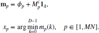
In Equation (10.36), we derived the min-sum equation in vector form, which we represent here as
These three equations completely describe the BP algorithm. However, to transform the equations into circuits, we need to add numerous constraints and sometimes modify the original intentions slightly. The first equation signifies iterations for message updation, although the iteration index is not shown. The second equation signifies the message vector at equilibrium, after suitable iterations. The third equation shows the process in which the optimal disparity is extracted from the message vector.
In this equation, the belief message m is originated from the pdf p:
In the design, the message must be represented by a finite word length. For stereo matching with D disparity levels, the belief vector is defined by
Thus, the messages can be interpreted as scoring functions for the desirable disparity at a pixel. In the circuit design, we further process the messages numerically to prevent overflow and underflow and to secure normalization. After undergoing more numerical transformations, the scoring values further become a sort of preference order. The operations between such vectors may transform from linear operations to nonlinear operations. In the design, the vector must be represented by an array either in packed or unpacked format.
According to the formula, a node p receives four belief vectors from its neighbors,
and outputs another four belief vectors to its neighbors
The subscript denotes the pixel positions, which may be absolute or relative. The four neighbors are represented by the relative positions, 0, 1, 2, and 3, referring to east, south, west, and north, encoded in clockwise direction. Conversely, the current pixel is represented by the absolute coordinate, ![]() . The message matrix must also be represented by an array, which is multidimensional.
. The message matrix must also be represented by an array, which is multidimensional.
Let us now design this algorithm with Verilog HDL, by adding more operations and also modifying the original algorithm appropriately to suit the nature of the numerical computation. The first step is to represent the belief message, m, in B bits: m ∈ [0, 2B − 1]. The word length must be enough to uniquely identify D disparity levels and thus, B ≥ log D. However, in actual applications, the entropy of the message is much smaller than log D and needs a much smaller word length. The determination as to the word length actually depends on the statistics of the application. Generally, the upper bound of B is log D. A fair decision on the word length may rely on the perplexity (Wikipedia 2013),
for a sufficiently large number of messages.
The next step is to define the normalization on this data. Because the belief value was derived from the probability, it must satisfy
Because of the finite word length and the smallness of D, this condition is not met exactly. Nevertheless, the message has already lost the meaning of probability and instead stands for relative magnitude between vector elements. Therefore, there are numerous ways of defining normalization for the belief message. One practical operation is to subtract the minimum from all the elements to make the elements unbiased. This operation is necessary because the message values may diverge due to continuous positive bias during the iteration.
The other operation is to amplify the messages so that the magnitude variation is maximal, consuming as many of the bits in B as possible. Otherwise, the distinction between vector elements may become vague due to small variances. To achieve this, let
where
If α is small, it means that the message variation is small and therefore we can use a lower number of bits, B, to code the message value. If α is large, we have to use a large B. The message variation depends on the problems, which require adaptive values for the word length B. Because we are concerned with hardware design, the word length is assumed to have been determined appropriately and fixed.
The output message matrix, Mo, is the state memory with which the subsequent states are determined, along with the input images. The circuit needs to store the message matrix in an array. There are several key points to bear in mind in representing the message matrix. The message matrix is not for a single pixel but for the entire image plane and is also defined for the four output message vectors. The storing of the messages is the main bottleneck in designing the BP. Usually, the spatial complexity in BP is O(MND). (In graph cuts, the spatial complexity is O(MN).) To represent the message matrix we may use small windows, m × n, which is much smaller than M × N, and use either a packed array or an unpacked array. The packed array is convenient for communicating data between modules but needs a field that is too long in the packed part: BD bits. Conversely, the unpacked array needs only B bits in the packed field but must be aided by counters for data communications. Considering all things together, let us represent the message matrix in an unpacked array but represent the incoming message in a packed array, so that the various operations in the combinational circuit can be more easily designed. This requires conversions from unpacked to packed and vice versa, which can be done with combinational circuits.
14.2 Window Processing
The basic platform for the BP algorithm is the FVSIM, in which full frame operations are available, as shown in Figure 14.1. The system consists of three buffers, storing two images (Il, Ir) and a disparity map D, and a circuit for computing the BP algorithm. The sizes of the three buffers are all M × N RGB pixels. The BP circuit is the main engine that reads the two images, computes the disparity, and stores the result in the disparity map. Unlike the buffers in the line-based algorithms, the buffers here are all full-sized frames.
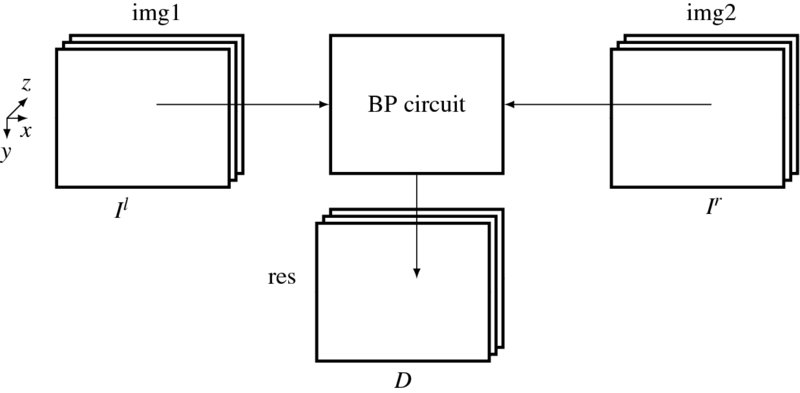
Figure 14.1 The components of the BP system. The three buffers, img1, img2, and res, respectively, store Il, Ir, and D. The BP circuit reads the two image buffers, computes the disparity, and then stores the result in the disparity buffer
In the BP circuit, the major data structure is the belief message matrix, M = {Mo(x, y)|x ∈ [0, n − 1], y ∈ [0, m − 1]}, for an m × n window. The total size is m × n × 4 × D, which is the bottleneck of the computation. To design the circuit, we have to restrict the window size, m × n, to meet the available resources.
Therefore, the BP circuit is based on window processing. The working window is illustrated in Figure 14.2. The image plane can be scanned in two opposite directions, as shown. The first type is the raster scan and is used in the right reference system, where the reference image is the right image plane. The second type is the opposite of the raster scan and is useful for the left reference system, where the reference coordinates are for the left image plane. A window is a rectangular area comprising m × n pixels. It is characterized by the origin, (x, y), defined by the top left corner (right mode) or the top right corner (left mode), and by the coordinates inside the regions. In addition, it is characterized by the shift intervals xs and ys between consecutive rectangles. If xs < n or ys < m, the windows are overlapped; otherwise, they are not overlapped. The coordinates inside the region are defined by (xx, yy), as shown. (Note that xx is a single variable.) Therefore, a window W(x, y) is a set of points, {(xx, yy)|xx ∈ [0, n − 1], yy ∈ [0, m − 1]}. This definition is adopted because it is convenient to locate the conjugate points in the other image. For the type 1 scan, the conjugate pair is (Ir(x + xx, y + yy), Il(x + xx + d, y + yy)), where the disparity d ≥ 0. Similarly, for the type 2 scan, the conjugate pair is (Il(N − 1 − (x + xx), y + yy), Ir(N − 1 − (x + xx + d), y + yy)) also d ≥ 0.
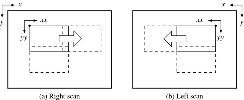
Figure 14.2 The frame, window, and scan directions
Associated with each window is the belief matrix, M(x, y) = {Mo(xx, yy)|xx ∈ [0, n − 1], yy ∈ [0, m − 1]}, where Mo(xx, yy) = (m(0), m(1), m(2), m(3)), indicating east, south, west, and north output belief vectors. A belief vector is a set of D belief messages, m = (m(0), m(1), …, m(D − 1))T, where D is the disparity level. The message m is encoded in a B bit binary number, as explained in the previous section.
The window scheme is quite general in that it can represent a pixel, m × n = 1, a line 1 × N in a row, a line in a column, M × 1, or the entire image plane, M × N. There is also freedom in the amount of overlap between contiguous windows. Reusing previous values is equivalent to the use of boundary conditions on the local windows.
14.3 BP Machine
Using the data representation and window processing in the FVIM framework, we can build a BP machine that computes the BP operations, as shown in Figure 14.3. The illustration shows the major constructs and operations of the machine. For the sake of clarity, the circuits are drawn only for the right reference system. For the left reference system, the role of the images must be switched. The top four elements are the memories, M(x, y) for the belief matrix at the window W(x, y), (Ir, Il) for the images, and D for the disparity map. They are the inputs and state memories. The other constructs are the sequential and combinational circuits, in which actual operations are executed. At a given time period, the memories are all fixed and the values in the combinational circuits are actively decided. Blocked at two sites, Mo and m, and connected by the combinational paths between the state memory and the blocking registers, the system as a whole becomes a finite state machine (specifically, a Mealy machine).
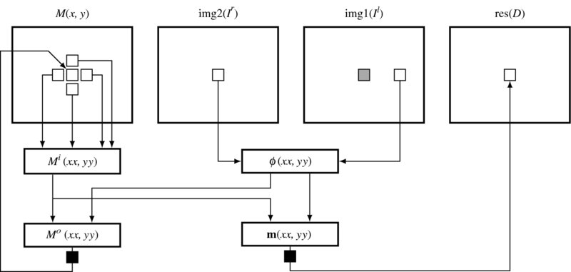
Figure 14.3 The flow of computation in the BP machine. Right reference mode. Two places are terminated by pipelining registers
In one period, all the computation is done for a pixel (xx, yy) in a window. The first step is to construct the input message matrix Mi by reading the state memory M. The vectors in the input matrix are the components of the four neighbors in the state memory. In parallel with the input matrix, the data vector is also composed from the image pairs. Combining the input message matrix and the data vector, we can build the output message matrix, following some extensive computations, as we will see. The determined matrix is held until the next clock. Eventually these data are overwritten to the state memory at the position (xx, yy), replacing the old one with the new one. Unlike the other parts, this section is realized with a sequential circuit. This cyclic process is repeated for a predetermined number of times and then the stabilized values in M and the data vector are used to build the message vector, m. The argument of the minimum element is the quantity that we are seeking and thus is to be stored in the buffer. The contents of the buffer are the disparity map.
14.4 Overall System
On the basis of Figure 14.3, let us now begin to design the Verilog HDL code. The header contains the parameters that characterize the images and the BP algorithm.
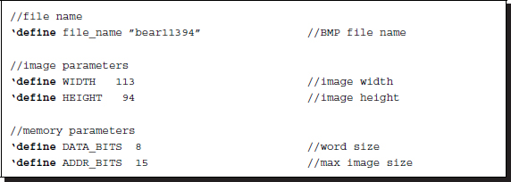
Listing 14.1 The header (1/12)
The filename is used for the IO part of the simulator to open and read the image files in the RAM, imitating the camera output. The image size, defined by the height and the width, M × N, is used to specify the required resources throughout the circuit. The memory parameters specify the word length and the address range for the contents in the RAM. The image data is ordinarily stored in bytes – three bytes for RGB channels. These parameters are also used to define the arrays, img1, img2, and res.
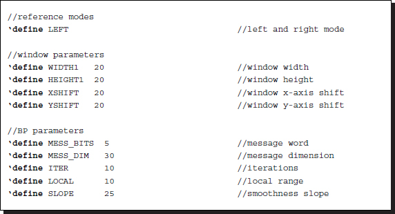
The next parameter is the key indicating the left or right reference modes. The window and the scan directions vary, depending on this parameter (Figure 14.2). The window parameters comprise the window width, height, horizontal shift, and vertical shift. The shift amount must be less than or equal to the window size. Otherwise, there will be empty regions in the disparity map.
The BP parameters specify the word length of the message, the number of states, the slope of the smoothness function, and the iteration number. The message length and dimension are important parameters as they determine the performance, the computational speed, and the space. The larger values may be better for better performance but they also require more space and computation. The message dimension must be the maximum disparity range, which can be observed only after experimentation. The message word length must be enough to encode the smallest and the largest messages. This decision is also possible only after observing the computation. The bits must be enough to uniquely differentiate the disparity levels, 2B ≤ D. This gives us, B ≤ log D. Usually, most of the disparities are labeled with the same index, making B ≪ log D. The most important factor determining the window is the belief matrix, which has a complexity of 4mnBD bits. The disparity size D is usually over 30, and thus the space complexity is overwhelmingly large to be applied to an entire frame. For larger disparity and message word, the window size must be small to be implemented in a chip. Next comes the smoothness function, which is characterized by the slope and local range and is the truncated linear function. The product of the slope and the local range must not exceed the maximum number range. More advanced algorithms may be implemented for the smoothness function, replacing the slope with appropriate parameters, such as the Potts model. Finally, the iteration number must be chosen so that the computation process reaches a stable state, at which time the disparity is determined as the index of the belief vector.
The main part of the code is as follows:
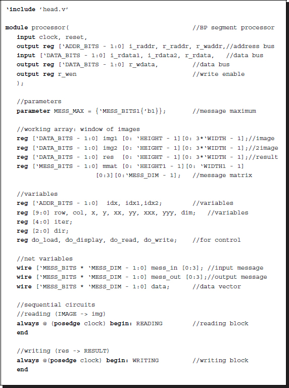
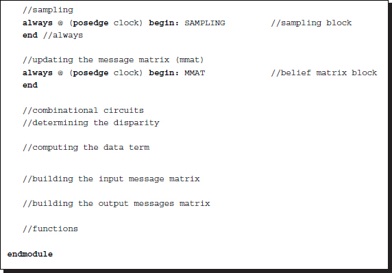
Listing 14.2 The framework: processor.v (2/12)
The code consists of three parts: sequential circuits, combinational circuits, and functions. The sequential part consists of four concurrent parts: reading, writing, sampling, and updation. The reading and writing blocks are the IP interfaces to the external RAMs, RAM1, RAM2, and RES, and the internal buffers, img1, img2, and res. The sampling block controls the window by moving around the image plane. This is common to both the left and right reference modes. Finally, the updation block writes the updated output message vector to the belief matrix, M. In this code, the message matrix is encoded as an unpacked array, mmat (refer to the problems at the end of this chapter). However, the message vectors, mess_in and mess_out, and the data vector, data, are all coded in packed format for computational simplicity (refer to the problems at the end of this chapter).
While the sequential part works for each clock tick, the combinational part works between the clock period, reading the data from the registers and stabilizing the result, so that in the next clock tick the result can be stored in the registers. The combinational part consists of four sections: a circuit building the input belief matrix, another building the data term, another building the output message matrix, and a circuit for determining the final disparity. The combinational circuits are aided by various functions, which all work in the same simulation time.
The components filling this template are explained in the following sections.
14.5 IO Circuit
Two of the sequential circuits are for reading and writing. The image data are located in the external RAMs, outside of the main processor, and must be accessed periodically. The circuit can be designed as follows.
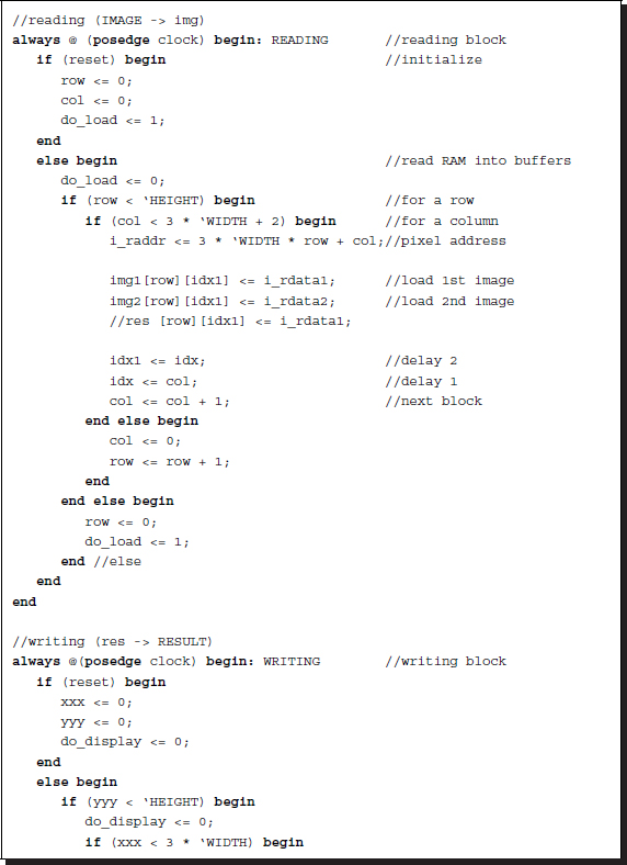
Listing 14.3 The IO circuit (3/12)
The purpose of the reading part is to read RAM1 and RAM2, and possibly RES into the internal buffers, img1, img2, and res. The processor reads the images Il and Ir from img1 and img2, processes them to determine the disparity, and writes the result into res, which finally stores the disparity map, D. To pair the address and data, some small delays must be introduced in the address bus. A mismatch exists between the incoming data and the current address, as the current data corresponds to the address two clocks ahead. These problems can be solved by the delay buffers idx and idx1 and the two-clocks delay in the address loop.
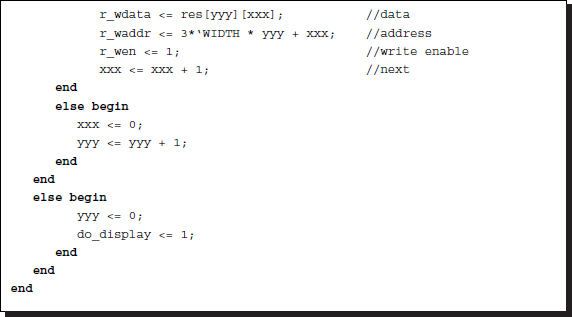
Another concurrent always block is the writing block. The purpose of this block is to write the disparity map, stored in the buffer, res, into the external RAM, RESULT, in RGB format so that the simulator can display the disparity map in BMP format. The flags, do_load and do_display, are used to control the simulator and therefore are not part of the synthesis. Note: the counters representing pixel positions ![]() ,
, ![]() ,
, ![]() , and
, and ![]() are all differently redefined in different always blocks in order to avoid multiple drivers for a net variable.
are all differently redefined in different always blocks in order to avoid multiple drivers for a net variable.
The remaining circuit can be considered a system that receives img1 and img2 as inputs and produces res as output.
14.6 Sampling Circuit
The computation is based on the window processing. A circuit that relocates the window around the image plane must be present. The constraint is that as a consequence of window movement, the entire image plane must be completely scanned, without producing empty spaces. In actuality, the space to be scanned is (x, y, l), where ![]() and l ∈ [0, L − 1] for some maximum iteration L. There is an algorithm that scans in the iteration index, called FBP (Jeong and Park 2004; Park and Jeong 2008). For hierarchical BP (Yang et al. 2006), sampling in this space must be made in the pyramid form. The order of the visit may be deterministic or random. In this chapter, we follow the usual approach, scanning of the image plane in a raster scan manner.
and l ∈ [0, L − 1] for some maximum iteration L. There is an algorithm that scans in the iteration index, called FBP (Jeong and Park 2004; Park and Jeong 2008). For hierarchical BP (Yang et al. 2006), sampling in this space must be made in the pyramid form. The order of the visit may be deterministic or random. In this chapter, we follow the usual approach, scanning of the image plane in a raster scan manner.
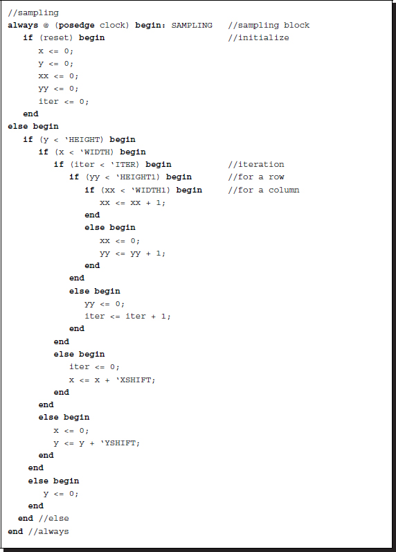
Listing 14.4 The sampling circuit (4/12)
In iteration notation, the circuit spans the M × N × L × m × n space in a ![]() manner, where xx is changed most rapidly and y is changed most slowly. Other iteration methods are also possible. The sampling circuit guides the window so that the image plane may be scanned in a certain way with counters. The amount of skipping in the horizontal and vertical directions is specified by the parameters, xs (XSHIFT) and xy (YSHIFT). The circuit has to generate three types of counters for the purpose: the window position on the image plane, the pixel position in a window, and the iteration number. With the auto-incrementing counter, x ≤ N − 1 and y ≤ M − 1, the window is positioned by the top left corner, (x, y), for the right reference mode and the top right corner, (N − 1 − x, y), for the left reference mode. Inside the window, the pixel is positioned by the counter, xx = 0, 1, …, n − 1 and yy = 0, 1, …, m − 1. Therefore, the absolute positions of the pixel are
manner, where xx is changed most rapidly and y is changed most slowly. Other iteration methods are also possible. The sampling circuit guides the window so that the image plane may be scanned in a certain way with counters. The amount of skipping in the horizontal and vertical directions is specified by the parameters, xs (XSHIFT) and xy (YSHIFT). The circuit has to generate three types of counters for the purpose: the window position on the image plane, the pixel position in a window, and the iteration number. With the auto-incrementing counter, x ≤ N − 1 and y ≤ M − 1, the window is positioned by the top left corner, (x, y), for the right reference mode and the top right corner, (N − 1 − x, y), for the left reference mode. Inside the window, the pixel is positioned by the counter, xx = 0, 1, …, n − 1 and yy = 0, 1, …, m − 1. Therefore, the absolute positions of the pixel are ![]() and
and ![]() , respectively, for both reference systems.
, respectively, for both reference systems.
The amount of overlap between two contiguous windows is determined by the window size and the shift parameter. In both directions, the overlapped regions are N − xs and M − ys. To be seen through the contiguous windows, suitable schemes for the boundary conditions must be considered. One way is to store the previous results around the boundary so that the next window can use them. The results may be the disparity values or the belief values. The other option is to use the data so that each window is independent of the other window processing. The former method needs a complicated scheme for storing the previous values, to use them in later windows, but leads to better performance. The latter scheme is the simplest of all but may result in poor performance around the window boundary.
The sampling scheme naturally involves a high degree of freedom, which is governed by the three counters, shift amount, and boundary policy. Here in the template, we consider only the basic one, two types of scanning, no overlap, and an independent window free from boundary preservation (see the problems at the end of this chapter).
In any case, the most important thing is that all the computation is described in terms of the current position and the time period. The current position is (xx, yy) in the message matrix and the current iteration is ![]() . The current position is
. The current position is ![]() for the right reference system and
for the right reference system and ![]() for the left reference system.
for the left reference system.
14.7 Circuit for the Data Term
From here onwards, all the computations are realized with combinational circuits, unless otherwise stated. The data vector, φ, is the major source of the belief message, driven by the input images, and thus must be provided accurately (Figure 14.3).
The concept for the provision of this vector is drawn in Figure 14.4. As shown in the figure, the sources of the data vector are the two image frames. The location of the current pixel is indicated as a position in a window, which is not shown here. A specific field, d, of the data vector is constructed by the data read from the two images. Therefore, a data vector can be constructed concurrently for all the pixels of the two images on the same epipolar line. All the elements of the vector are determined by the combinational circuits as follows.
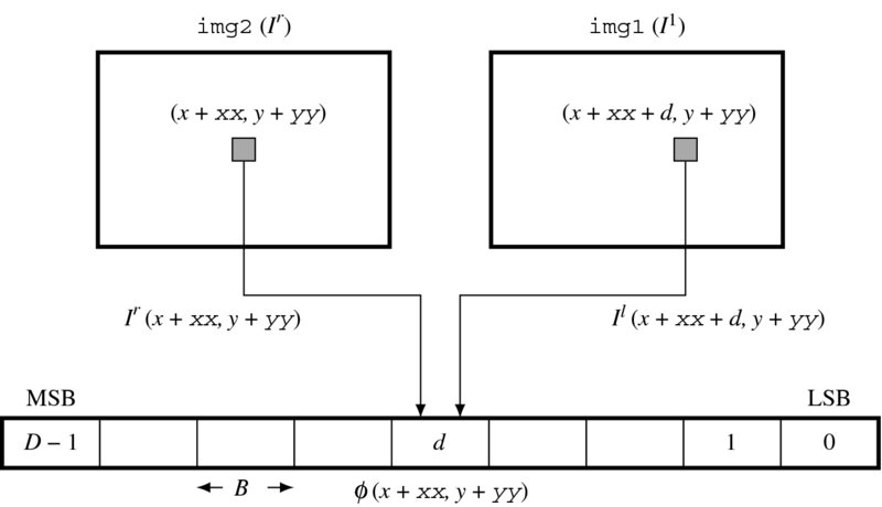
Figure 14.4 Building the data vector,  , where (x, y) is the window position and
  is the pixel position within the window. The vector is generated by the combinational circuits for all elements in parallel
The data vector is encoded in a packed array of BD bits, because it must often be accessed as one complete set of data (see the problems at the end of this chapter). In the right reference system, the data term is
where φD − 1 is the MSB and φ0 is the LSB. Each element is a B bit number with
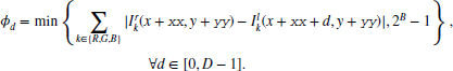
Here, the data value is limited within a B bit word length, preventing overflow.
For the left reference system, the data are defined as
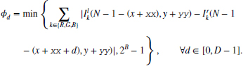
Advanced algorithms may use different schemes for computing the data term, for example, with better distance measure and maybe an occlusion indicator. This code is a basic template that contains only the most basic features.
Keeping in mind the concept, one can code the algorithm as follows. (Because there are a lot of identical circuits, the Verilog generate construct is used. The code also contains the Verilog compiler directive to switch the design between the two reference modes.)
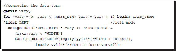
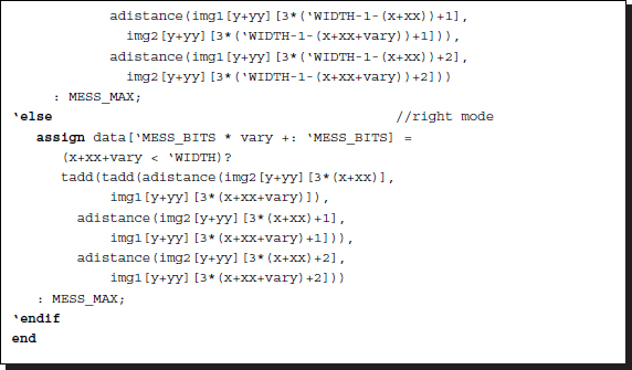
Listing 14.5 The data term (5/12)
The circuits are compiled separately according to the two types of reference systems. Each reference system consists of D continuous assignments, with each assignment determining a B bit field in the data vector. The circuits are generated by the Verilog HDL generate construct. Consequently, this part of the circuit consists of D combinational circuits.
Two functions are used in the expression: adistance and tadd. Function adistance is an absolute function that returns the absolute distance between two arguments. Function tadd is an addition that accounts for saturation math. The upper bound of the truncation is defined as 2B − 1. The functions, together with other functions, will be discussed in later sections.
Knowing the distribution of elements in a vector is very important, because the data vector is to be combined with message vectors. If either of the two vectors dominates the other, the combined result may be less efficient. This is part of the reason for normalizing the messages, as will be seen. Considering the sum of three differences in the RGB channels, the range of φ is between 0 and 255 × 3. To limit the number in B bits, which are used for message encoding, the data vector must also be normalized appropriately. This issue is also postponed to a later section.
14.8 Circuit for the Input Belief Message Matrix
The input message vector must be constructed in parallel with the data vector because they are combined soon afterwards (Figure 14.3). For this purpose, the required circuit is to build Mi in Equation (14.3) out of Mo.
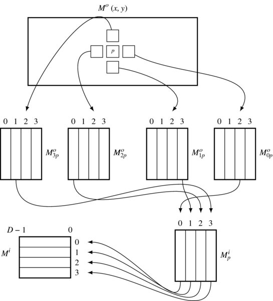
Figure 14.5 Building the input belief message matrix at 
The concept is depicted in Figure 14.5. Consider that the current position is ![]() , with (x, y) for the window and
, with (x, y) for the window and ![]() for the pixel within the window. At this window, the input belief matrix, Mi(x, y), is decided. First, take the output belief matrix from the four neighbors, as shown in the figure. Each matrix contains four vectors, indicating four directions. Next, extract a vector from each matrix, west for east, north for south, east for west, and south for north vector, as shown, and build a matrix, Mip. The matrix is in the ordinary set of four vectors and thus must be converted to the packed array form.
for the pixel within the window. At this window, the input belief matrix, Mi(x, y), is decided. First, take the output belief matrix from the four neighbors, as shown in the figure. Each matrix contains four vectors, indicating four directions. Next, extract a vector from each matrix, west for east, north for south, east for west, and south for north vector, as shown, and build a matrix, Mip. The matrix is in the ordinary set of four vectors and thus must be converted to the packed array form.
This can be explained precisely with equations. In Equation (14.1), this stage corresponds to the computation: Mip. Consider a position ![]() . At this position, we are going to build the input matrix:
. At this position, we are going to build the input matrix:
The neighbors at p have the output matrices:
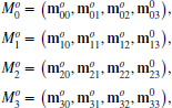
where all the subscripts are the relative directions, east, south, west, and north. Extracting a vector from each matrix, we can construct the input matrix:
The criterion for choosing an element is based on the neighborhood. For example, the east input must be the west output of the east neighbor and the north input must be the south output of the north neighbor.
Although this seems complicated, the core operation is just reading and building the matrix in packed array format. The circuits consist of only four continuous assignments. Considering the D fields, we need to generate 4D combinational circuits.
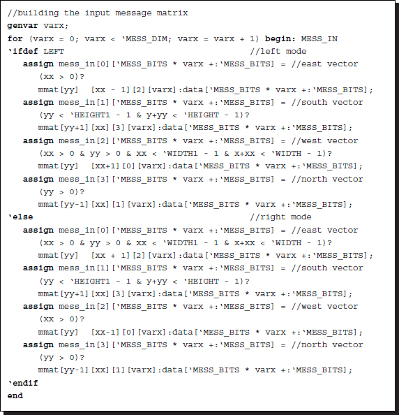
Listing 14.6 The input message matrix: processor.v (6/12)
In addition to choosing the vectors and rotating them into packed field format, the circuit must also account for the boundary conditions. Around the image boundary, one or two neighbors may be missing. There are two kinds of boundaries: the window boundary and the image boundary. The neighbor may be out of the window but within the image frame. In another case, the neighbor may be completely outside the image frame.
One method is to replace the belief with the data terms. That is, for the first kind of neighbor, the belief is replaced with the data term in that pixel. For the second kind of neighbor, the belief is replaced with the data term of the current pixel. In effect, the image is expanded with the boundary values. Using this method, the windows are independent of each other and glued by the data terms. We will follow this approach to make the circuit simple. In the code, this concept is reflected as the conditional statements. A more sophisticated method that stores the actual messages, instead of using the data terms, and reuses them later in other windows is possible. This kind of strategy is needed for better performance and iteration over the entire image plane, following the iteration inside the window.
Note that the code is separated with the Verilog compiler directive for the right and left reference modes. The difference between the two modes is the use of the counters for computing the coordinates. For the right mode, the conjugate point is on the right and for the left mode, the conjugate point is on the left.
14.9 Circuit for the Output Belief Message Matrix
Given the data vector and message matrix, we can design the main circuits for generating the output message. This part is the most complicated circuit, where the variance between the data term and the message term, as well as the variance between messages in a message vector, must be properly regulated. Moreover, the smoothness function must be applied and the operation of minimum selection must be introduced. This operation requires four stages: selective averaging, adding of data terms, adding of smoothness function, and choosing the minimum. These complicated operations must be aided by the specialized functions.
In Equation (14.1), the output message matrix has the form
where
for a matrix A and vector b. Let Mop = (mo0, mo1, mo2, mo3) and x = Φ + Mip(141T4 − I4 × 4). Then, the expressions mean
where ⊙ means that the vector elements satisfy
Because Ψ is already known and stored as parameters, this operation can be designed into a function, mess_min, which receives a vector and produces the desired output. This function is one of the most complicated in the BP circuit, as we will see.
To design the circuit, we divide the equation into several stages, as illustrated in Figure 14.6. In the first stage, three of the input vectors are selected and then added to the data vector. This is realized with the function mess_4av in the Verilog HDL code. This function operates field by field to take the average of the four elements.
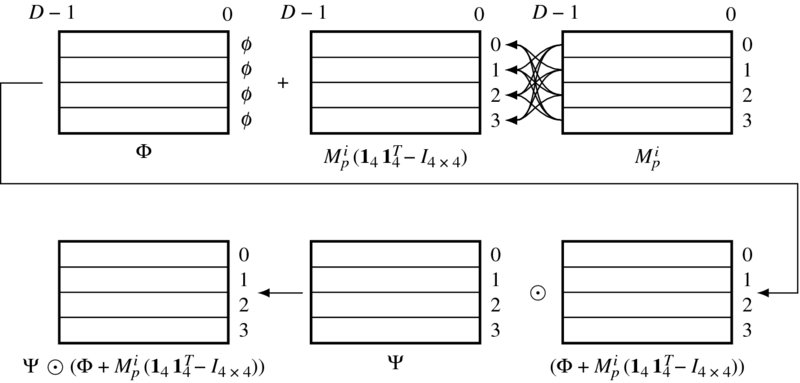
Figure 14.6 Building the output message matrix
In the second stage, the vectors are weighted with a smoothness function and the minimum elements are chosen. This is realized by the function mess_min. The functions will be discussed in more detail in a later section.
The actual code is as follows.
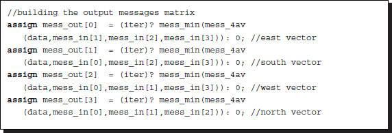
Listing 14.7 The output belief matrix (7/12)
The four output vectors are independently generated by calling the function mess_min. In the code, the initialization is also encoded. At the start, which can be recognized by the first iteration, the message matrix must be initialized. In this case, the initial values are all the same, zero. However, other values may be used instead of zero.
14.10 Circuit for the Updation of Message Matrix
The output matrix is overwritten to the current position of the output message matrix. This operation must be sequential, storing the result until the next clock, because the path from Mo(x, y) to the output message matrix is a combinational path. The formats of M and Mo are different: M is encoded and unpacked while Mo is encoded in packed array format. Therefore, the message format must be transformed from packed to unpacked array before updation.
This operation is realized by the following circuit.
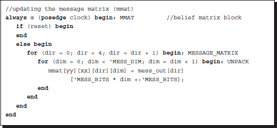
Listing 14.8 The framework: processor.v (8/12)
In the code, each field is read and written to the vector element. The iteration is converted to 4D different circuits.
14.11 Circuit for the Disparity
The operations between the input message matrix and the output message matrix form a cycle. The iteration is aimed at a convergent system. Eventually, when the iteration ends, the message matrix M must be used for the final operation, which is to determine the disparity from the message vector and to write it to the result buffer. In Equation (14.1), the corresponding operation is
This can be realized by two functions: mess_4av and argmin. Function mess_4av takes the average of the four vectors, while function argmin chooses the argument of the minimum element. The concept is depicted in Figure 14.7. In the figure, Mi is the input belief message matrix at a point. The matrix is reduced to a vector by mess_4av. This vector is then added to the data vector at this pixel by another average function, mess_av. From the vector, the minimum and corresponding index, which is the optimal disparity at this pixel, is computed.
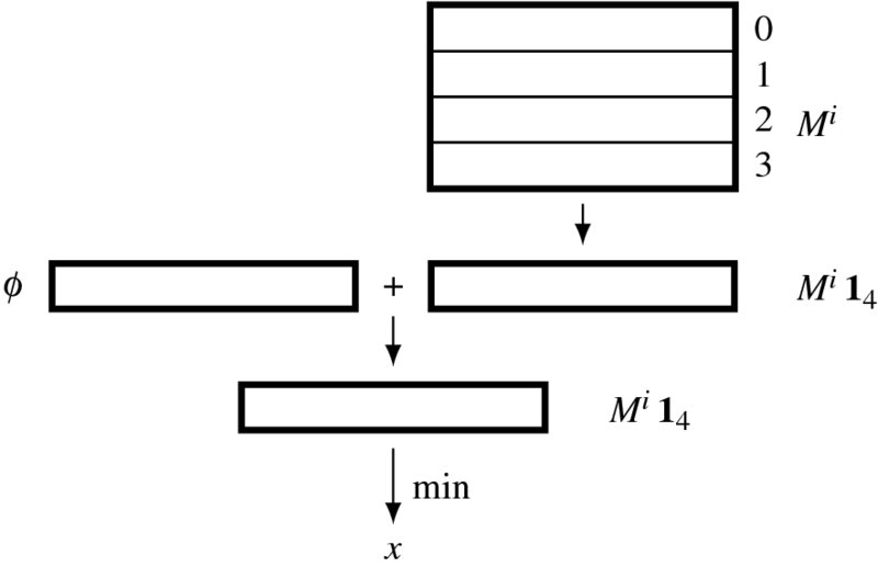
Figure 14.7 Building the result vector
The operations are designed by the following code.
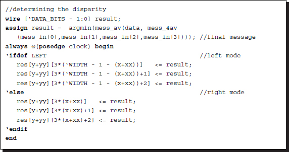
Listing 14.9 The framework: processor.v (9/12)
The major operation is realized with the combinational circuit. However, an additional sequential operation is needed for terminating the flow of the combinational circuit and writing the vector to the internal buffer, res, at each clock tick. The buffer finally stores the disparity map. For the BMP display, the disparity map is copied into three channels.
14.12 Saturation Arithmetic
Thus far, the combinational circuits are aided by many functions, and are a compact method of writing the common codes in the function. The restriction is that the codes must be executed within the same simulation time and the variables should all be local. Due to the variable scopes, accessing the entire image or message matrix is very inefficient. Let us design the circuits for such functions.
The first function is tadd, which adds numbers limiting the size within the predefined bounds. Usually, the lower bound is zero and the upper bound is the full field: 2B − 1, where B is the word length of the message. This operation must be secured so that underflow and overflow are avoided. All the other functions using any kind of addition may use this saturation math.
The second function is mess_av, which takes two vectors in packed array form and takes averages field by field. This function uses the truncated addition mentioned above. Function mess_4av is an expansion of mess_av from two to four variables. The function computes the average of the four vectors, using mess_av twice.
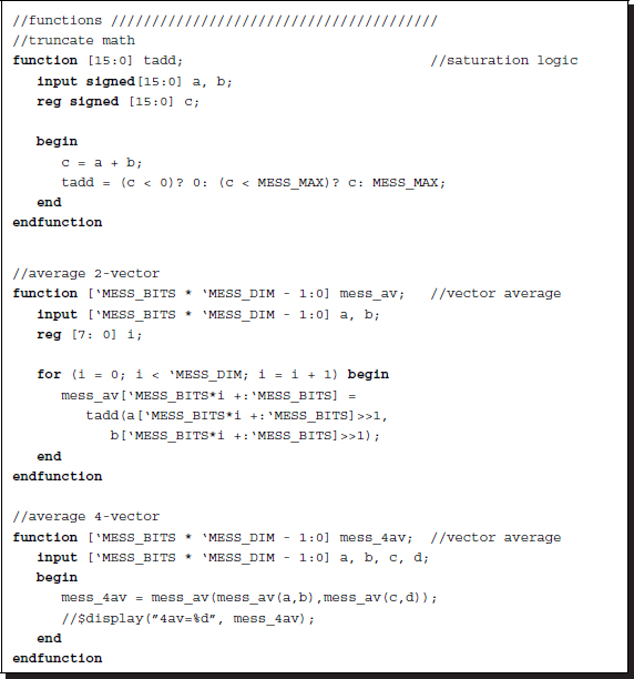
Listing 14.10 The functions (10/12)
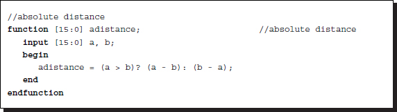
As well as the additions, difference operations are needed to measure the likelihood of two numbers. The basic distance between two numbers is defined by the absolute distance, although other advanced distance measures can replace this. The function, adistance, works for this purpose, in an integer word length.
14.13 Smoothness
The output message uses the function mess_min, as described in Equation (14.18). For a given vector x and the function, ψ, the function evaluates
In the Verilog design, the vectors are all represented by packed arrays. The smooth function is predefined and thus may not be supplied as an additional argument to the function.
The underlying concept of the circuit is illustrated in Figure 14.8. The input vector is a message vector among the four, represented in packed array. The D weighted message vectors, y, are obtained by weighting with D different smooth functions. The smoothness function here is the truncated linear model but can be any model, such as the quadratic model or the Potts model. Each field of the intermediate vector, ![]() , is obtained by selecting the minimum of the corresponding weighted vector. This vector undergoes some more processes, collectively called normalization.
, is obtained by selecting the minimum of the corresponding weighted vector. This vector undergoes some more processes, collectively called normalization.
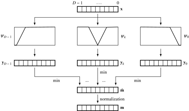
Figure 14.8 Building an output belief message vector with the operations: weighting (truncated linear), minimum selection, and normalization
In the following, the concept is coded in Verilog HDL.
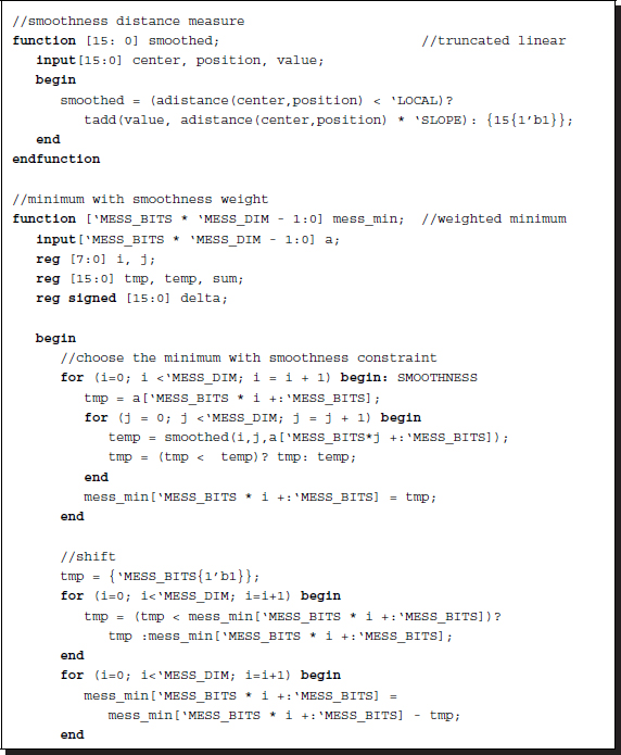
Listing 14.11 The functions (11/12)
For the weighting, ψ + x, a function, called smoothed, is defined. The given vectors x and the smoothness vector ψ in this function evaluate
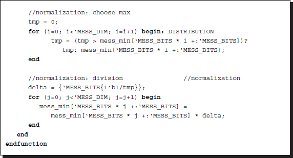
Function mess_min computes Equation (14.20) in two steps: minimum selection of the weighted vector and normalization. For the first operation, the circuit uses smoothed. The normalization stage involves a number of sequential stages. The first stage shifts the element down to base zero:
This operation is necessary because the message may be increased during the BP operations to the upper bound, 2B − 1, threatening overflow. The normalization starts with the selection of a maximum number. Subsequently, all the elements are divided by the common divisor so that the message is in the range [0, 2B − 1].
Observing the statistical distribution of the message values, we may notice that the dynamic range is very small and thus the full B bits may not be necessary. In fact, the nature of the images and the applications, and the chosen smoothness function, all contribute to the message distribution (see the problems at the end of this chapter). In some cases, normalization may not be necessary. From the given template, we can further develop circuits that are more efficient in both complexity and performance.
14.14 Minimum Argument
After the iteration is complete, the messages are supposed to be in equilibrium. At this instant, the final message is determined and, thus, the disparity. This is the concept of the original theory. In actuality, the circuit executing this task is separate from the circuit for the message updation and is thus concurrent, as are the other circuits. Therefore, there is no reason to halt this circuit during the iteration.
In Equation (14.1), the corresponding operation is
Function argmin returns the argument of the minimum given the input vector.
In the Verilog HDL, this operation reads:
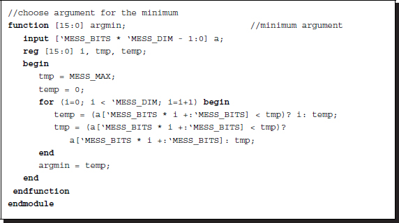
Listing 14.12 The functions (12/12)
It is important to choose the minimum near the center position when multiple minima exist throughout the elements in a vector. This is because the required value is not the message but its index, which must be as near to the current position as possible. An appropriate weight must be designed so that this condition is guaranteed. Otherwise, the circuit must be redesigned in a more complicated manner.
14.15 Simulation
Let us observe the testing of the BP circuit. The test images used were a pair of 225 × 188 images (CMU 2013; Middlebury 2013). They can be seen at the top of Figure 14.9, with the lower images being the disparity maps. The parameters for the BP were as follows. The window size was 40 × 40 and was moved un-overlapped in raster scan manner. Each window was iterated 10 times, somewhat earlier than complete convergence. The smoothness function was the truncated linear function with slope 25 in a 10 pixel range. Beyond the range, the smoothed value was saturated to the upper bound.
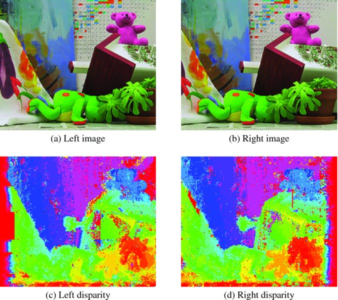
Figure 14.9 Disparity maps (image size: 225 × 188, disparity level: 32, window size: 40 × 40, iteration: 10, truncated linear function: 25)
The right reference map had a poor region at the right side. In like manner, the left reference map had a poor region at the left side. Compared to the disparity map obtained by the DP machines, the result was less noisy, even if the result was not yet fully saturated. There were some remnants, some of the marks of the windows, due to the window processing. To avoid such window traces, the windows must be overlapped slightly around boundaries. The major differences between the two disparity maps are the important clues for computing occluding regions.
In complexity view, the BP machine needed 4mnDB bits to store the message matrix and MNT time for computation, where T signifies iteration. Compared with the DP O(N2D) for a single processor and O(N) for the D processor array, the BP consumed more space and time than DP but generally gives better results. The competitive algorithm, graph cuts, gives similar results, but takes less space, O(MN), though the control structure is more complicated. It is known that the two algorithms have evolved in this direction: BP gets faster and GC gets more general.
Problems
- 14.1 [Data representation] A message is represented by the scoring function. If the abstraction process continues further, the message loses its meaning as a probability and score function. Instead, the quantities in the message vector will relate to preference order. Thus, m = (m0, m1, …, mD − 1, where m ∈ [0, D − 1]. In such a case, what are the proper operations that correspond to the addition and average?
- 14.2 [Overall system] How is the message matrix, mmat, represented in packed form?
- 14.3 [Overall system] How can a message be sent in the packed and unpacked forms for the message matrix mmat?
- 14.4 [Overall system] In the code, the message and data vectors are coded in a packed array in contrast to the message matrix, which is in an unpacked array. Represent the message and data vectors in unpacked forms. Discuss their advantages and disadvantages.
- 14.5 [Overall system] In Listing 14.2, the message matrix was defined for disparity computation. What is the equivalent matrix representation for optical flow? Discuss using the spatial complexity. For instance, let the velocity vector (u, v) and their limits be U_DIM and V_DIM. For disparity, the message matrix is

In the disparity matrix, the spatial complexity is 4mnDB bits. For the optical flow, the message matrix has spatial complexity comprising UV, where U and V are the limits of u and v.
- 14.6 [Overall system] In Listing 14.2, the IO and sampling circuits are separately designed. Build a circuit that combines the three into one using an FSM.
- 14.7 [Sampling circuit] In Listing 14.4, the space is scanned in a (y(x(l(xx))) manner, where xx changes most rapidly and y changes most slowly. What other scanning methods could be used?
- 14.8 [Data term] In Listing 14.5, the neighbors outside the window are assigned data along the boundary. However, we instead want to expand the outside in mirror image. Change the data term for such a mirror image case. Actually, there can be many more cases, which may need more computation. This modification is provided for the right mode only. However, similar changes can be made for the left mode also.
- 14.9 [Input message matrix] In Listing 14.6, the outside neighbors are bounded by the data on the boundary. Change the code so that the mirror image is used instead for the neighbors around the boundary.
- 14.10 [Functions] In Listing 14.10, the average of vectors is defined for the packed array. Modify the operation for an addition.
- 14.11 [Functions] In Listing 14.11, the distance measure is absolute. The Potts model is often more robust in many noisy environments. Design a function for the Potts model.
References
- CMU 2013 Cmu data set http://vasc.ri.cmu.edu/idb/html/stereo/ (accessed Sept. 4, 2013).
- Felzenszwalb P and Huttenlocher D 2004 Efficient belief propagation for early vision Proceedings of the 2004 IEEE Computer Society Conference on Computer Vision and Pattern Recognition, pp. I261–I268 number 1.
- Grauer-Gray S and Kambhamettu C 2009 Hierarchical belief propagation to reduce search space using CUDA for stereo and motion estimation In Proceedings of 2009 Workshop on Applications of Computer Vision, pp. 1–8.
- IEEE 2005 IEEE Standard for Verilog Hardware Description Language. IEEE.
- Jeong H and Park S 2004 Generalized trellis stereo matching with systolic array Lecture Notes in Computer Science, vol. 3358, pp. 263–267.
- Jian S, Zheng N, and Shum H 2003 Stereo matching using belief propagation. IEEE Trans. Pattern Anal. Mach. Intell. 25(7), 787–800.
- Klaus A, Sormann M, and Karner K 2006 Segment-based stereo matching using belief propagation and a self-adapting dissimilarity measure ICPR (3), pp. 15–18. IEEE Computer Society.
- Liang C, Cheng C, Lai Y, Chen L, and Chen H 2011 Hardware-efficient belief propagation. IEEE Trans. Circuits and Systems for Video Technology 21(5), 525–537.
- Middlebury U 2013 Middlebury stereo home page http://vision.middlebury.edu/stereo (accessed Sept. 4, 2013).
- Montserrat T, Civit J, Escoda O, and Landabaso J 2009 Depth estimation based on multiview matching with depth/color segmentation and memory efficient belief propagation 16th IEEE International Conference on Image Processing, pp. 2353–2356.
- Park S and Jeong H 2008 Memory efficient iterative process on a two-dimensional first-order regular graph. Optics Letters 33, 74–76.
- Stankiewicz O and Wegner K 2008 Depth map estimation software version 2 ISO/IEC MPEG meeting M15338.
- Szeliski RS, Zabih R, Scharstein D, Veksler OA, Kolmogorov V, Agarwala A, Tappen M, and Rother C 2008 A comparative study of energy minimization methods for Markov random fields with smoothness-based priors. IEEE Trans. Pattern Anal. Mach. Intell. 30(6), 1068–1080.
- Taguchi Y, Wilburn B, and Zitnick C, 2008 Stereo reconstruction with mixed pixels using adaptive over-segmentation CVPR, pp. 1–8.
- Tippetts BJ, Lee DJ, Archibald JK, and Lillywhite KD 2011 Dense disparity real-time stereo vision algorithm for resource-limited systems. IEEE Trans. Circuits Syst. Video Techn 21(10), 1547–1555.
- Tippetts BJ, Lee DJ, Lillywhite K, and Archibald J 2013 Review of stereo vision algorithms and their suitability for resource-limited systems http://link.springer.com/article/10.1007%2Fs11554-012-0313-2 (accessed Sept. 4, 2013).
- Wikipedia 2013 Perplexity http://en.wikipedia.org/wiki/Perplexity (accessed Sept. 2, 2013).
- Yang Q, Wang L, Yang R, Stewenius H, and Nister D, 2009 Stereo matching with color-weighted correlation, hierarchical belief propagation, and occlusion handling. IEEE Trans. Pattern Anal. Mach. Intell. 31(3), 492–504.
- Yang QX, Wang L, and Yang RG 2006 Real-time global stereo matching using hierarchical belief propagation BMVC, p. III:989.
- Yedidia J, Freeman W, and Weiss Y 2003 Exploring Artificial Intelligence in the New Millennium Morgan Kaufmann Publishers Inc. chapter Understanding Belief Propagation and Its Generalizations, pp. 239–269.
- Yu T, Lin R, Super B, and Tang B 2007 Efficient message representations for belief propagation ICCV, pp. 1–8.