
6
Stereo Vision
Binocular stereo vision is one of the major vision modules by which one can induce the depth of the surface shape and the volume information of the objects. Created by a pair of cameras, a conjugate pair of images contains the depth information by means of disparity. Binocular vision naturally expands to other vision, such as trinocular or multi-view vision (Faugeras 1993; Faugeras and Luong 2004; Hartley and Zisserman 2004).
Stereo vision deals with the three major problems: correspondence geometry, camera geometry, and scene geometry. Of these, stereo matching deals with the correspondence geometry and remains the major research area. It can be classified into various categories according to the features, measures, inference methods, and learning methods. A comprehensive survey of recent progress on stereo matching is presented by (Scharstein and Szeliski 2002) for algorithms, and by (Tippetts et al. 2013) for realizations. Also, they have provided a benchmark for quantitative evaluation of existing stereo matching algorithms.
This chapter introduces some fundamental concepts of stereo vision problems and stereo matching. Instead of reviewing all the extensive stereo matching algorithms and realizations, we focus instead on the fundamental constructs of the energy function, classified as appearance model and geometric constraints. The models and constraints are examined in five categories: space, time, frequency, discrete space, and other vision module. Stereo matching, as other vision problems, is inherently ill-posed, and thus needs the best possible natural constraints. Unfortunately, all the constraints are not sufficient and necessary conditions but are always accompanied by exceptional cases. This is why the study of natural constraints must be emphasized compared to others. The actual algorithm uses constraints, features, measures in energy function and optimization methods and parameter estimation methods in a variety of ways.
The contents are not intended to be complete in their scope and depths but intended to be a good preparation for the topics in subsequent chapters. In particular, a baseline form of energy function is expressed, which will be used in later chapters for the study of computational structure and circuit design.
6.1 Camera Systems
Projective geometry (Faugeras 1993; Faugeras and Luong 2004; Hartley and Zisserman 2004) is one of the three components of the image formation process, along with the illumination and reflectance properties. Since stereo and motion deal with images and videos, knowing the optical environment is important to describe various vision quantities mathematically. First, we must know the mechanism of projection from object to image plane. Next, the relationship between world coordinates and image coordinates must be specified in detail.
In a perspective model (or pinhole model) camera, the image plane is positioned behind the lens center, in inverted direction. (Figure 6.1(a).) The camera coordinates are denoted by Oc, which is called the center of projection (or optical center). An image plane ![]() is positioned at a distance f, which is called focal length. Here, the center of the image, o, is the origin of the image coordinates. A point P in the 3-space is projected, through Oc, on the image plane
is positioned at a distance f, which is called focal length. Here, the center of the image, o, is the origin of the image coordinates. A point P in the 3-space is projected, through Oc, on the image plane ![]() , forming an image p in an inverted and scaled shape.
, forming an image p in an inverted and scaled shape.
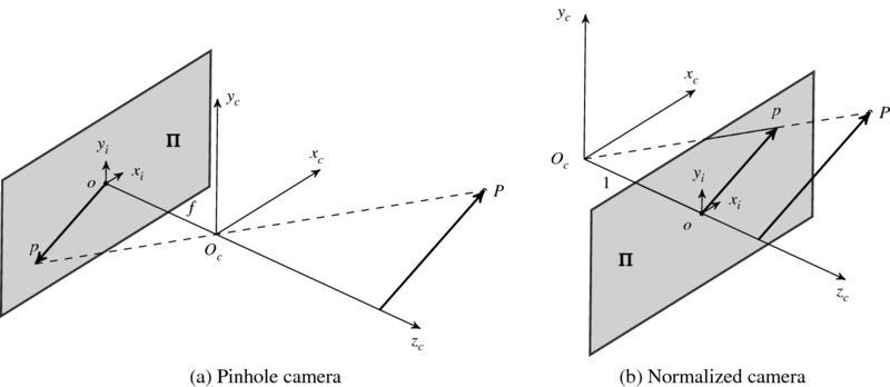
Figure 6.1 Two camera systems: pinhole and normalized cameras
The inverted image is inconvenient and thus often represented in a different scheme, in which the image is positioned in the same direction as the object. The scheme is to consider a virtual image plane that is located before the lens so that the coordinates of camera and image are overlapped in the depth direction. This scheme, especially with f = 1, is called normalized camera (Figure 6.1(b)). The fronto-parallel plane ![]() at the focal length, f, in front of the xcyc-plane is called the virtual image plane. The principal plane is the plane that includes the optical center. The principal point, o, is where the principal axis zc and the plane
at the focal length, f, in front of the xcyc-plane is called the virtual image plane. The principal plane is the plane that includes the optical center. The principal point, o, is where the principal axis zc and the plane ![]() coincide. We often use the normalized camera, unless otherwise stated.
coincide. We often use the normalized camera, unless otherwise stated.
In Cartesian coordinates, a point ![]() is projected to the point
is projected to the point ![]() , satisfying
, satisfying
which means that the system is perspective.
In projective geometry, using homogeneous coordinates is essential, because it makes perspective projection a linear transformation. In 2D space, a point ![]() in inhomogeneous system (Cartesian,
in inhomogeneous system (Cartesian, ![]() ) is represented by x = [x, y, 1] in homogeneous system (
) is represented by x = [x, y, 1] in homogeneous system (![]() ). Inversely, a point x = [x, y, w] in homogeneous system is represented by
). Inversely, a point x = [x, y, w] in homogeneous system is represented by ![]() if w ≠ 0. (For simplicity, sometimes we use row vector instead of column vector.) In short, [x, y, w] ≡ (x/w, y/w) if w ≠ 0. In 3D space, a point
if w ≠ 0. (For simplicity, sometimes we use row vector instead of column vector.) In short, [x, y, w] ≡ (x/w, y/w) if w ≠ 0. In 3D space, a point ![]() in inhomogeneous system (
in inhomogeneous system (![]() ) is represented by x = [x, y, z, 1] in homogeneous system (
) is represented by x = [x, y, z, 1] in homogeneous system (![]() ). Inversely, a point x = [x, y, z, w] in homogeneous system is represented by
). Inversely, a point x = [x, y, z, w] in homogeneous system is represented by ![]() if w ≠ 0. In short, [x, y, z, w] ≡ (x/w, y/w, z/w) if ≠ 0.
if w ≠ 0. In short, [x, y, z, w] ≡ (x/w, y/w, z/w) if ≠ 0.
The algebraic properties are summarized as follows. For vector addition, [x, y, z] + [a, b, c] = [za + xc, zb + yc, zc]. For scalar multiplication, a[x, y, z] = [ax, ay, z], where a ≠ 0. For linear combination, α[x, y, z] + β[a, b, c] = [zβα + αxc, zβb + αyc, zc]. For derivative, d[x, y, w] = [dx, dy, w].
In geometric interpretation, ![]() is spanned by (1, 0) and (0, 1), but
is spanned by (1, 0) and (0, 1), but ![]() is spanned by [1, 0, 1], [0, 1, 1], and the ideals: x∞ = [1, 0, 0] and y∞ = [0, 1, 0], called point at infinity, and l∞ = [0, 0, 1], called line at infinity. However, [0, 0, 0]T does not represent any point. Excluding [0, 0, 0, 0],
is spanned by [1, 0, 1], [0, 1, 1], and the ideals: x∞ = [1, 0, 0] and y∞ = [0, 1, 0], called point at infinity, and l∞ = [0, 0, 1], called line at infinity. However, [0, 0, 0]T does not represent any point. Excluding [0, 0, 0, 0], ![]() consists of the bases ([1, 0, 0, 1], [0, 1, 0, 1], [0, 0, 1, 1]), the ideals (x∞, y∞, z∞, π∞). The same concept can be expanded to
consists of the bases ([1, 0, 0, 1], [0, 1, 0, 1], [0, 0, 1, 1]), the ideals (x∞, y∞, z∞, π∞). The same concept can be expanded to ![]() and
and ![]() and further higher dimension. (For further information on projective geometry, refer to (Faugeras and Luong 2004; Hartley and Zisserman 2004).)
and further higher dimension. (For further information on projective geometry, refer to (Faugeras and Luong 2004; Hartley and Zisserman 2004).)
According to the homogeneous coordinates, Equation (6.1) becomes
In the following, the notations of row and column vectors and of the coordinates are used interchangeably and the actual meaning must be clear from the context.
6.2 Camera Matrices
A discrete image is often modeled as an array of N × M pixels: I = {I(x, y)|x ∈ [0, N − 1], y ∈ [M − 1]}, where the origin of the image is the north-west corner of the array, like a matrix. Conceptually, such a discrete image is obtained from a continuous image, I(x, y), x ∈ [ − a, a], y ∈ [ − b, b], where a and b are image sizes. Therefore, the two formats are related, with coordinate transformation such as translation and scale change. Moreover, the camera image must be related to world coordinates, for the camera is positioned and oriented in 3-space. Besides, the object itself has coordinates. Considering all these together, we will need the five coordinates system: (x, y) for the pixel coordinates, (xc, yc) for the image coordinates, (xc, yc, zc) for the camera coordinates, (xo, yo) for the object coordinates, and (X, Y, Z) for the world coordinates. In Figure 6.2, the five coordinates systems are represented by the origins and the projected points. In this optical alignment, P is observed as (X, Y, Z) in world coordinates, (xo, yo, zo) in object coordinates system, (xc, yc, zc) in camera coordinates system, (xc, yc) in image coordinates system, and (x, y) in pixel coordinates system.
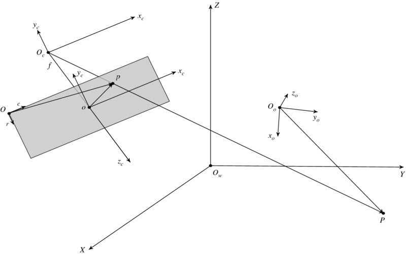
Figure 6.2 Coordinates systems: pixel (O), image (o), camera (OC), object (Oo), and world coordinates (Ow)
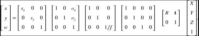
The coordinates transformation from world to pixel plane can be described by linear mapping, provided that homogeneous coordinates are adopted. The mapping consists of the four stages: from object to world, world to camera, camera to image, and image to pixel image. (The object coordinates are ignored for simplicity.) The mapping from world to camera is an orthographic projection in 3D that can be specified by the rotation matrix R3 × 3 and the translation vector t3 × 1. The mapping from camera to image is a perspective projection, which is specified by the focal length f. The mapping from image to pixel is a mapping specified by the translation (ox, oy) in pixels and scaling by the effective size of the pixel, (sx, sy), in the horizontal and vertical direction, respectively. As such, an image point, (x, y), can be related to the object point, (X, Y, Z), in the world coordinates in the following way. To differentiate between homogeneous and inhomogeneous coordinates, let
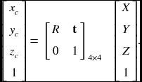
In general, the world and camera coordinates have the relationship, which is described by rotation R and translation t. In homogeneous coordinates systems, the relationship is linear, xc = [R|t]X:
The projection from camera to image coordinates is described by perspective transformation: xi = diag(1, 1, 1/f)[I|0]xc:
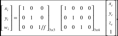
where the dimension is reduced and the scale is reduced by the focal length f. The mapping from image xi to pixel x is expressed by
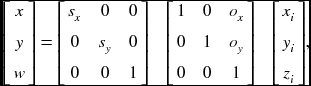
where (sx, sy) are scale factors (isotropic if equal and anisotropic if unequal), and (ox, oy) is the offset between image and pixel planes.
The overall combination of Equations (6.4), (6.5) and (6.6) becomes
We represent this by
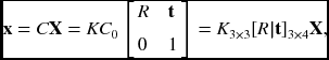
where C, C0, and K are respectively called the camera matrix, canonical form, and calibration matrix. The calibration matrix has the form:
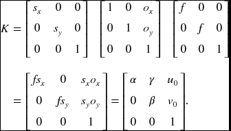
Here, α and β denote focal length in terms with pixels, γ (often zero) denotes skew coefficient.
The normalized camera matrix CN is defined by
This is equivalent to the camera in which the focal length is unity, the origin is centered on the image, and the scale is unity. Thus the intrinsic parameters are removed and only the extrinsic parameters are retained. This camera is often the starting point when only the extrinsic parameters must be considered.
Conceptually, the camera matrix consists of three vanishing points and the projection of world origin:
Let x∞ = [1, 0, 0, 0]T, y∞ = [0, 1, 0, 0]T, and z∞ = [0, 0, 1, 0]T be ideals and O = [0, 0, 0, 1]T be the world origin. Then, we have
where the first three vectors represent respectively the x, y, and z vanishing points and the last represents the projection of the world origin.
In general, the image plane may be transformed from 2D to 2D, so-called homography: x = Hx′ with x′ = CX. Then, the general expression is x = HCX and thus the general camera matrix C′ is the product of homography and camera matrix:
The camera matrix expresses the 3D to 2D transformation including rotation, translation, perspective, scaling (isotropic or anisotropic), and offset. The homography expresses the 2D to 2D transformation, meaning 2D rotation, 2D translation, 2D perspective, and 2D scaling (isotropic or anisotropic).
Excluding homography, the overall system can be described by (K, R, t). In particular, the parameters in (R, t) called extrinsic parameters and consist of six parameters. The parameters in K is called intrinsic parameters and consists of five parameters. As a result, the system consists of a total of 11 parameters.
6.3 Camera Calibration
Determining the parameters given the image and scene points is called camera calibration. Among many, the three major approaches are: direct linear transformation (DLT) method (Dubrofsky 2007; Hartley and Zisserman 2004), Roger Y. Tsai algorithm (Tsai 1987), and Zhang's method (Zhang 2000).
The DLT supposes that {(xk, yk), (Xk, Yk, Zk)|k ∈ [1, K]} is the set of 2D-3D pairs. From Equation (6.8),
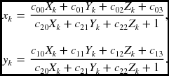
This equation becomes
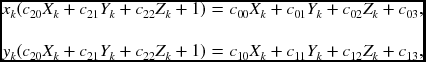
which can be solved by linear regression methods such as least squares or pseudo-inverse. Since 11 parameters are unknown and two equations are available per point, six points are sufficient, though more points may be better for making the system over-determined.
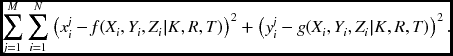
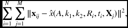
The parameters can be determined by solving nonlinear equations (Tsai 1987). The 2D coordinates are just a nonlinear function of its 3D coordinates, expressed with camera parameters:
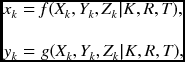
where f and g are the nonlinear functions, derived from Equation (6.8). Consider that we are given N points in each of M images: {(xji, yij)|i ∈ [1, N], j ∈ [1, M]}. The parameters can be estimated by the nonlinear optimization:
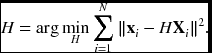
Once we have recovered the numerical form of the camera matrix, we still have to separate out the intrinsic and extrinsic parameters. This problem is not an estimation problem but a matrix decomposition such as SVD. The parameters can also be obtained by using the homography method (Zhang 2000). Suppose the corresponding pairs are x and X.
Let Z = 0, then
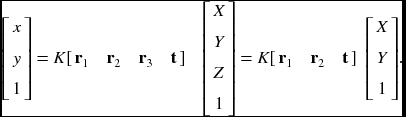
Therefore, the homography is H = K[r1, r2, t], which can be estimated by the given N corresponding pairs:
Given the homography, H = [h1, h2, h3], we can compute the intrinsic parameters by solving
where λ is a scale factor. Since the rotation matrix R is orthonormal, r1 and r2 in Equation (6.21) satisfy
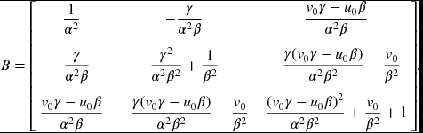
Let B = K− TK− 1, then from Equation (6.18), B becomes
Now let's simplify Equation (6.21) by vector products. Since B is symmetric, we can represent it by the upper diagonal elements, b = [B11, B12, B22, B13, B23, B33]T. For H, define h = [h11h21, h11h22 + h12h21, h12h22, h13h21 + h11h23, h13h22 + h12h23]T. Then, Equation (6.22) becomes
From this, we obtain the following variables first,
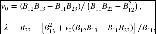
then the remaining parameters,
Next, let's solve for the extrinsic parameters. From Equation (6.21),
Besides, we may need more parameters, such as radial distortion (de Villiers et al. 2010; Weng et al. 1992). Let (x, y) and (x′, y′) be ideal and real image coordinates. Let (x, y) be ideal normalized image coordinates and (x′, y′) be real normalized image coordinates. Then, we have
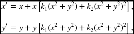
where k1 and k2 are distortion parameters. In the pixel domain, (u, v) is the ideal pixel image coordinates and (u′, v′) is real observed image coordinates. Then,
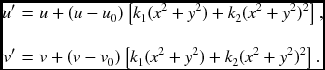
This equation can be represented by Dk = d, or
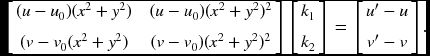
The pseudo-inverse is k = (DTD)− 1DTd. If we are given M images with N points each, we can solve this by linear least squares estimation (LLSE). Combining the homography and the distortions, we have the complete LLSE:
where ![]() means the projective transform with the intrinsic and extrinsic parameters.
means the projective transform with the intrinsic and extrinsic parameters.
There has been extensive research on camera calibration (Brahmachari and Sarkar 2013; Chin et al. 2009; Hartley and Li 2012; Ni et al. 2009; Rozenfeld and Shimshoni 2005; Zheng et al. 2011). OpenCV (OpenCV 2013) contains standard camera calibration programs that find intrinsic and extrinsic para- meters, together with distortions.
6.4 Correspondence Geometry
If more than two cameras are used to capture the same scene, there exist some constraints for the points in the same image and for the corresponding points in different images. Such constraints play key roles in restoring three-dimensional information.
In stereo vision, the major problems are classified into these three: correspondence geometry, camera geometry, and scene geometry. The correspondence problem is to study the topic: given an image point in the first view, how does it constrain the corresponding point in the second view? The camera geometry is the problem: given a set of corresponding points, what are the cameras matrices for the two views? The scene geometry is the problem: given corresponding image points and cameras matrices, what is the position of the point in 3D? To answer such problems, we have to understand the geometry of the stereo system.
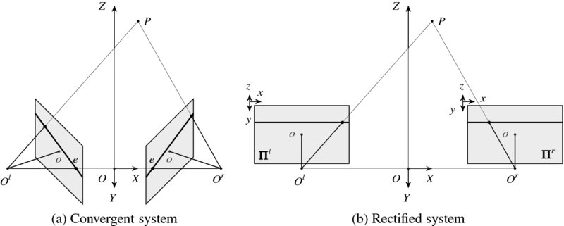
Figure 6.3 Stereo camera systems: convergent and rectified systems
The binocular vision system consists of two cameras aligned as in Figure 6.3(a). The points, Ol and Or, are respectively the projection centers of the left and right cameras. The common focal length is f. In this alignment, a point P forms a plane POlOr, which is called the epiplane. The lines on the images, called epipolar lines, are the projection of the pencil of planes passing through the optical centers. Therefore, ![]() and
and ![]() . The point e, called the epipole, is where the projection center of the other camera is mapped on the image plane. Therefore,
. The point e, called the epipole, is where the projection center of the other camera is mapped on the image plane. Therefore, ![]() and
and ![]() .
.
If the camera system is aligned in such a way that two optical axes are parallel, the system looks like Figure 6.3(b). The images in this system are called rectified images, which are often the starting point of the stereo matching. The image planes are coplanar and the epipolar lines are collinear and thus the search for matching points becomes a one-dimensional search problem. The rectification process is to convert the convergent system to the rectified system by coordinate transformations.
Let's observe how different points in 3-space generate different epipolar lines in the image convergent and rectified planes. Figure 6.4 shows the epipolar lines generated by the points at different heights. In the rectified image, the epipolar lines are always parallel and the epipole is at infinity at the same height, el = er = ∞. Furthermore, the row of an epipolar line is the same as the y-axis of the camera image. In such a rectified system, a 3-space point appears on both epipolar lines which are in the same epiplane. On the other hand, in a convergent system, all the epipolar lines pass through an epipole, e, forming a set of rays. In this system, too, an object point appears on the corresponding epipolar lines in both images.
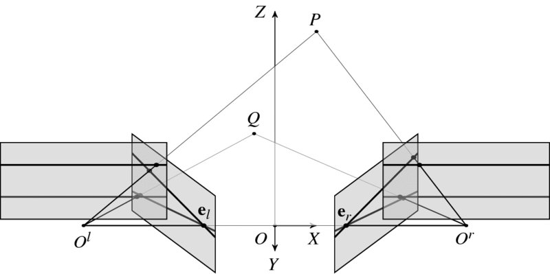
Figure 6.4 Epiplanes, epipolar lines, and epipoles for two points
Let's derive the relationship between corresponding points (Figure 6.5). In this figure, pl and pr are a conjugate pair, ll and lr are epipolar lines, and el and er are epipoles. A point P is observed as Pl and Pr on the left and right cameras and pl and pr on the left and right images, respectively. The object point and the image point are all related by
If the right system is translated and rotated with respect to the left system by the rotation matrix R and translation vector t = (tx, ty, tz)T, then the vector on the left system is observed in the right system as
Since the three vectors, Pl − t, t, and Pl, are all on the same epiplane, the following relationship must hold:
Since RTR = I,
Combining the front two factors into one, we have
which with Equation (6.33) becomes
Substituting Equation (6.32) into (6.37) yields

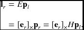
where [t]× is a skew symmetric matrix representing the cross product-conversion to matrix representation of the cross product with t. (We sometimes use T instead of [t]×.) That is, for two vectors a and b, the cross product becomes a × b = [a]×b. The relationship, called essential matrix E, was first derived by (Longuet-Higgins 1981). Conceptually, this equation means that in camera images the corresponding points must be on the same epipolar line. For a pair of conjugate points, (xl, yl) and (xr, yr), in the image plane, this equation specifies that yl = yr but doesn't specify the relation between xl and xr.
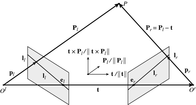
Figure 6.5 The geometry of two camera system
The essential matrix encodes information on the extrinsic parameters only. The essential matrix explains that the conjugates pair, pl and pr, is on the epipolar lines, ll = ETpr and lr = Epl, we have pTrlr = 0 and lTlpl = 0. Since pTrEel = 0 and eTrFpl = 0 hold for all pr and pl, respectively, Eel = 0 and ETer = 0. It has rank 2 since R is full rank but [t]× is rank 2. Its two nonsingular values are equal. The degree of freedom is 5. The essential matrix can be decomposed into the product of epipole and homography. Let
with the homography, H. Then, we get
Repeating for the epipolar line on the left image plane, we have
(See the problems at the end of this chapter.)
Suppose that p = [u, v, 1]T and p′ = [u′, v′, 1]T are a corresponding pair. For N ≥ 8 points, the essential matrix can be obtained by
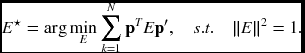
This can be transformed to the linear least squares estimation (LLSE). For the points and essential matrix, define the vectors: x = (uu′, uv′, u, vu′, vv′, v, u′, v′, 1)T and e = (e11, e12, e13, e21, e22, e23, e31, e32, 1)T. Then, Equation (6.38) becomes xTe = 0. For N ≥ 8 points, define X = (x1, …, xN). Then, the essential matrix can be estimated by
In this formula, the solution is the eigenvector associated with the smallest eigenvalue of eTe.
For the uncalibrated camera, this equation must be expressed in terms with the conjugate points in the pixel planes. Since the mapping from camera image to the pixel plane can be specified by a shifted, rotated, and scaled transformation by the calibration matrix K, the image point p and the pixel coordinates q are related by
Putting this into Equation (6.38) yields
This relation, called the fundamental matrix, was first derived by Luong (Faugeras et al. 1992; Luong and Faugeras 1996). Conceptually, this relationship means that in pixel images the corresponding points must be located on the corresponding epipolar lines. Likewise the essential matrix, for a pair of conjugate points, (xl, yl) and (xr, yr), in the pixel plane, this equation specifies that yl = yr but doesn't specify the relation between xl and xr. (See the problems at the end of this chapter.)
As opposed to the essential matrix, the fundamental matrix expresses some important properties of the uncalibrated camera system. The fundamental matrix encodes information both the intrinsic and extrinsic parameters. It has rank 2 due to E. It has seven degrees of freedom also up to scale. The lines Fql and FTqr represent the epipolar lines associated with pl and pr, respectively. Also, the epipoles are null points, satisfying Fel = 0 and FTer = 0.
6.5 Camera Geometry
The eight-point algorithm (Chojnacki and Brooks 2007; Hartley 1997; Longuet-Higgins 1981) is to determine the parameters with the known eight conjugate pairs. Suppose that q = (u, v) and q′ = (u′v′) are a corresponding pair. For N ≥ 8 points, the fundamental matrix can be obtained by
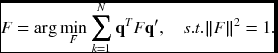
This can be transformed to the linear least squares estimation (LLSE). For the points and essential matrix, define the vectors: x = (uu′, uv′, u, vu′, vv′, v, u′, v′, 1)T and f = (f11, f12, f13, f21, f22, f23, f31, f32, 1)T. Then, Equation (6.38) becomes xTf = 0. For N ≥ 8 points, define X = (x1, …, xN). Then, the fundamental matrix can be estimated by
In this formula, the solution is the eigenvector associated with the smallest eigenvalue of fTf.
For a full description of the perspective projection and the relationship between cameras, all the matrices (i.e. C, E and finally R and [tx]) must be recovered, starting from F. From the recovered F, we can compute the singular value decomposition (SVD):
where U and V are lower and upper triangular matrices, respectively. We project the fundamental matrix onto the essential manifold:
The SVD of F contains the information on epipoles. The epipole e is a null vector, satisfying Fel = 0. Therefore, the epipole is the column of VT corresponding to the null singular value, VT = (v1, v2, el). Similarly, er satisfies FTer = 0 and thus the column of UT corresponding to the null singular value, UT = (u1, u2, er).
From the fundamental matrix, we obtain the essential matrix,
where σ = (σ1 + σ2)/2. The obtained essential matrix minimizes the Frobenius distance ‖E − F‖2.
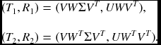
Once the essential matrix is obtained, the other matrices, E = TR, can be recovered by SVD (Hartley and Zisserman 2004):
where Σ = diag(1, 1, 0). Let's define the skew symmetric matrix, W− 1 = WT:
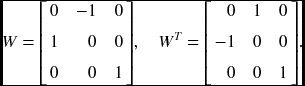
Then, there are two solutions:
6.6 Scene Geometry
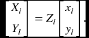
The scene geometry problem is to find X, given E and the corresponding pair, xl and xr. According to (Longuet-Higgins 1981), this problem can be solved as follows.
Let R = (rT1, r2T, rT3)T. For simplicity, consider that the world coordinates and the left camera coordinates coincide. The camera systems are normalized, with the essential matrix (R|t) and the corresponding pair is given by ![]() and
and ![]() . Between the recovered scene points,
. Between the recovered scene points, ![]() and
and ![]() , the following relationship holds:
, the following relationship holds:
The components are
Then, the image coordinates are ![]() :
:
From this, we get one element of the 3D coordinates:
Here, the scale factor f is restored. As a last step, the remaining element can be recovered by
Therefore, ![]() is recovered from
is recovered from ![]() and
and ![]() , with the help of (R|t)). Due to the inaccurate corresponding pair, Zl in Equation (6.57) may not be the same. In actual algorithm, the estimation error must be minimized for more than one corresponding pairs.
, with the help of (R|t)). Due to the inaccurate corresponding pair, Zl in Equation (6.57) may not be the same. In actual algorithm, the estimation error must be minimized for more than one corresponding pairs.
There is a common case, where the camera is positioned at (B, 0, 0), tilted with θ with respect to the baseline. The two cameras are focused at the point C, called the subject distance. In this common case, we have the explicit solution for the 3D position (Figure 6.6). The right camera is shifted by t = (B, 0, 0) and rotated by
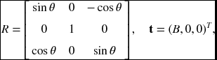
where θ is the angle between the optical axis and the baseline. In that case, Equation (6.58) is reduced to
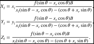
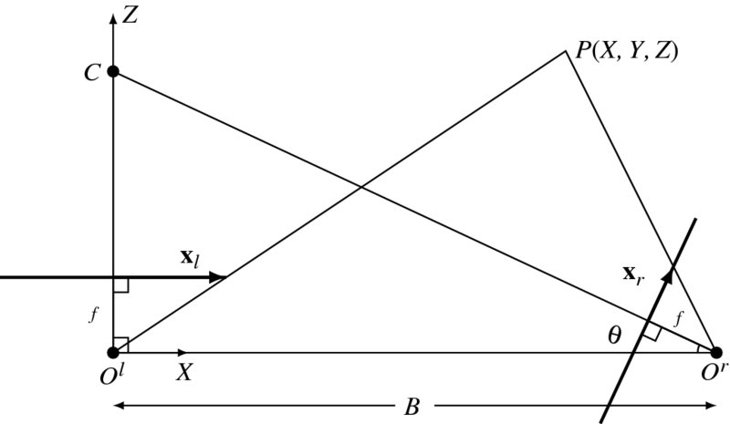
Figure 6.6 Cameras on the same plane: world and left camera coordinates coincide. The cameras are focused at the common point C (f: focal length and B: baseline.)
6.7 Rectification
In convergent systems, finding corresponding points is a 2D search problem because the epipolar lines are radiating lines on the plane. Rectification is a warping process via perspective transformation so that epipolar lines are horizontal. In a rectified system, the problem is a 1D search problem because the epipolar lines are all horizontally parallel. As such most stereo matching algorithms start with the premise: epipolar lines in the rectified system.
To see the relationship between the two systems, look at Figure 6.7. In this system, a set of points, {P, Ol, Or}, constructs an epiplane, POlOr, which intersect the planes of the convergent systems, producing epipolar lines in slanted directions. The rectified system can be achieved by rotating the convergent system around the projection center maintaining the focal length unchanged. The condition for the rotation matrix R is that in the rotated planes the epipolar lines should be collinear.
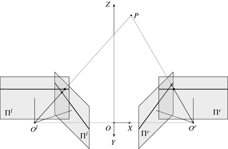
Figure 6.7 Two camera systems: rectified and convergent cameras
Let xTrFxl = 0. The problem is to find homographies Hl and Hr such that yl = Hlxl and yr = Hrxr, which satisfies yTrF′yl = 0. Solving this, we obtain
for the parallel camera.
There are basically three algorithms for image rectification: planar rectification (Fusiello et al. 2000; Trucco and Verri 1998), cylindrical rectification (Oram 2001), and polar rectification (Pollefeys et al. 1999). Planar rectification is as follows.
Assume that the system is normalized and the extrinsic parameters [R|t] are given. The first step is to rotate the left image plane so that the epipole goes to infinity along the horizontal line. Since the rotation matrix is orthonormal, only one vector can be specified and thereby we can derive the other two. The starting vector is conveniently decided by the epipole which is a foreshortened vector of the translation t between two camera coordinates. Thus, let the first vector, u = t/‖t‖. The other two vectors can be built as follows:
where u⊥ must satisfy u × u⊥ and the z-axis. Set the rotation matrices Rl = Rrect and Rr = RRrect for the left and right cameras. Once Rl and Rr are obtained, the points, q, in the rectified system can be obtained from the points, p, in the convergent system, according to
where pl = (xl, yl, zl)T and pr = (xr, yr, zr)T. As a consequence of rectification, the epipoles are all located at infinity el = er = ∞ and the epipolar lines are collinear ll × lr = 0.
After the transformation, the resulting image must be resampled and interpolated to compensate for the irregular empty pixels. (For further methods, refer to (Kang and Ho 2011; Loop and Zhang 1999; Miraldo and Araújo 2013; OpenCV 2013; Zhang 2000).)
The rectified system is a special case, shown in Figure 6.6. The right camera is positioned at (B, 0, 0), in parallel with the left camera. This is the most common framework for a rectified system (Figure 6.8). The right camera is shifted by t = (B, 0, 0) and thus θ = π/2 in Equation (6.60).
As a consequence of rectification, we have derived Equation (6.64). This standard configuration is called the epipolar plane model. In this alignment, a point P is projected on (xl, yl) for the left image and (xr, yr) for the right image. The two image points are collectively called corresponding points.
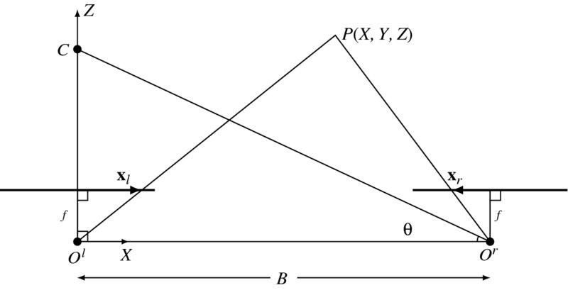
Figure 6.8 Rectified cameras: world and left camera coordinates coincide (f: focal length and B: baseline)
The Equations (6.64) can be conveniently described by the common variable,
which is called disparity. It satisfies always d ≥ 0 and configures the 3D positions by
Unlike in the rectified system, the depth is not a simple function of the disparity.
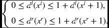
In Equation (6.66), the importance of disparity is self-evident; depth estimation becomes the disparity estimation problem. In this optical arrangement, xl ≥ xr ≥ 0. When we estimate the disparity, so-called stereo matching, one of the two image coordinates must be chosen as a reference. To distinguish the two cases, we define the left and right disparities:
Here, d ≥ 0, regardless of the reference systems. Since the mapping between the conjugate pairs is not a one-to-one mapping due to occlusion, the two quantities, dl and dr, are not generally the same. Knowing both dl and dr may help to determine the occluding area.
As a special case, if the world coordinates are located between the two cameras, we get
If the world coordinates coincide with the left camera coordinates, the 3D position is
6.8 Appearance Models
In a simple rectified system, 3-D positions can be recovered by the disparity in Equation (6.66). Otherwise, the scene geometry can be recovered by the conjugate pairs as mentioned previously. Therefore, the remaining problem is to find the conjugate pairs, so-called correspondence problem, and represent them with the disparity map. The constraint is that the conjugate pairs are on the epipolar line, as specified by the fundamental matrix. Stereo matching is the method for solving the correspondence problem.
To fulfill this goal, we need some measures to decide the features, distance measures, inference method, and learning method. The feature is a representation of the matching pixels and generalized from local to global descriptors. The candidate pairs are compared with the distance measures or other correlation measures. The matching error is represented by a constrained optimization problem, which can be resolved by many inference methods. Finally, all the parameters included in the optimization problem are often estimated by learning methods. Owing to the diversity of stereo matching, some taxonomy has been tried so far (Scharstein and Szeliski 2002).
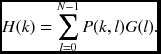
Numerous techniques and algorithms have been introduced for solving the constrained and unconstrained optimization of the stereo matching problem. However, there is still uncertainty of the bound of performance and the ground-truth solutions. The problem is not the technique for solving the problem but it seems to reside in the uncertainty in the modeling and the constraints for solving the ill-posed problem. In this context, instead of reviewing the vast methods, we focus on the more fundamental principles, called constraints, as they are close to the nature and building blocks of the optimization problem. The constraints together become the energy function, consisting of the data term D and the smoothness term V with the Lagrange multiplier:
Here, the disparity on the image plane is represented collectively by the disparity map. Depending on the reference coordinates, the disparity can be defined as left, right, or center disparity. As mentioned in Chapter 5, the general form consists of the appearance and geometric constraints, which will be addressed in this and following sections.
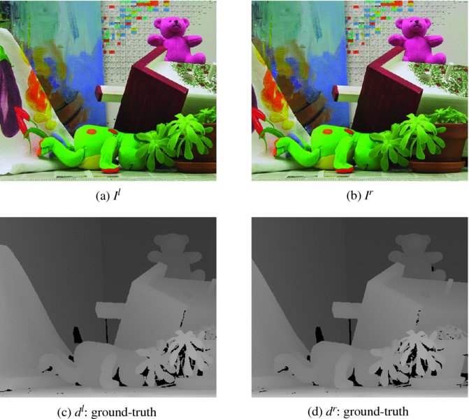
Figure 6.9 The stereo images and the ground-truth disparity map
As an example, the stereo images consist of a pair of left and right images (Middlebury 2013), as shown in Figure 6.9. The first two images are the left and right images. The next two images are the ground-truth disparity maps. The brightness shows the depth and the black segments show the pixels where the depth information is unavailable due to the sensor limitation. The ground truth is not the baseline of the disparity map but a reference, because a lot of the state-of-the-art algorithms, such as message passing, move-making, or LPR-based algorithms, tend to beat the ground truth.
The appearance model can be interpreted in many different ways: conservation laws, assignment error, observation error, unary potential, etc. Whatever the interpretation, the appearance model appears as a data term, relating the image and the putative disparity. One of the most prevailing laws is the photometric constraints (or intensity conservation or brightness conservation) of the corresponding points, which posits that the intensity of the same object is invariant in different views, assuming that they are spatially and temporally differentiable. This assumption results in the two equations:
For large variations of the disparity range, any series expansion of this function is inappropriate, unlike the series expansion that is possible for optical flow.
The two disparities are not always the same in general environment, because the disparities can be viewed as two different mappings. That is, dl: (x, y)↦(x + dl(x, y), y) and dr: (x, y)↦(x + dr(x, y), y). The error variance of the disparity is also increasingly deteriorated as the matching point approaches the boundary. For the right disparity, the mapping ranges is xr ∈ [0, N − 1]↦xl ∈ [xr, N − 1], and for the left disparity, the mapping range is xl ∈ [0, N − 1]↦xr ∈ [0, xl]. It is natural that the uncertainty of the disparity increases as the point approaches the boundary (right boundary for the right disparity and left boundary for the left disparity). On the other hand, the uncertainty is minimal on the other end of the boundary (left boundary for the right disparity and right boundary for the left disparity).
6.9 Fundamental Constraints
Unlike the epipolar hypothesis, other constraints are not always true. Although the brightness conservation is the natural choice of data term in the energy function, the problem is ill-posed in nature and thus needs more constraints to limit the search space. The geometric constraints fill such gaps, revealing the natural properties of the 3D geometry because a priori knowledge is possible. Because objects interact in time and space, there exist numerous geometric constraints. Let us examine the constraints, classified as space, time, frequency, segment, and 3D-based constraints.
Among the disparity-based constraints, the most fundamental constraint is the smoothness constraint, which means that the disparity of the neighboring pixels on an object surface must be as smooth (differentiable) as possible since the object surface is generally smooth. The smoothness measure assumes that if the surface is smooth, so do the disparity values:
This premise is also very difficult to justify, because the disparity is the result of two different views for the same surface and thus the slope and the boundaries may affect the disparity in a very complicated manner. The are many variations of this form in terms of the derivative order, neighborhood size, and truncated values. Among many others, the linear truncation and Pott's model are the most popular methods. This constraint holds only when the neighbors are on the same surface but not across the boundary. Enforcing this constraint tends to make the boundary smooth, losing the sharp transition, even when sophisticated surface fitting methods (i.e. membrane or thin plate) are adopted. To achieve anisotropic diffusion, these constraints must be supported by the estimation of surface, boundary, and occlusion.
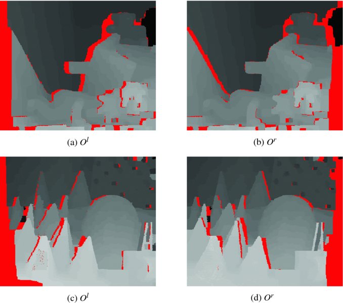
Figure 6.10 The occluding regions of the Teddy and Cones images
Another constraint is the occlusion, an invisible part of the scene for one of the two cameras. Examples are shown in Figure 6.10. The disparity maps contain occluding regions, particularly around object boundaries. Each disparity map, left or right, has its own occluding regions. Also, the occluding regions tend to be sparse and difficult to detect for small objects.
Knowing the occluding region can help the stereo matching drastically, because the smoothness can be suppressed in those areas, resulting in sharp boundaries and preventing smearing between adjacent regions. However, determining the occluding areas is a difficult problem, particularly when only one type of disparity map is available (Min and Sohn 2008; Tola et al. 2010; Zitnick and Kanade 2000).
Let O(p) represent an indicator function for the occlusion at ![]() . One way to define occlusion is to check the one-to-one correspondence (Bleyer and Gelautz 2007; Kolmogorov 2005; Lin and Tomasi 2003). We can classify the pixels into two classes: consistent (one-to-one mapping) and occlusion (many-to-one mapping). For
. One way to define occlusion is to check the one-to-one correspondence (Bleyer and Gelautz 2007; Kolmogorov 2005; Lin and Tomasi 2003). We can classify the pixels into two classes: consistent (one-to-one mapping) and occlusion (many-to-one mapping). For ![]() and
and ![]() , we define
, we define
The left/right occlusion map is an M × N binary image which is the collection of such sites. This constraint is also not strict, due to the slanted surfaces (Bleyer et al. 2010; Ogale and Aloimonos 2004; Sun et al. 2005). The occlusion can also be defined by (Woodford et al. 2009)
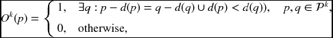
where k ∈ {l, r}.
The possible preservation of order might be a strong constraint in stereo matching. The distribution of disparities between neighbor pixels may be arbitrary in principle, but the order of pixels tends to be preserved in both image and disparity map. To see this, consider two consecutive pixels, xl and xl + 1, which have disparities, dl(xl) and dl(xl + 1), respectively. The corresponding pixels are xr = xl + dl(xl) and xr = xl + 1 + dl(xl + 1), respectively. Since xl < xl + 1, it is natural that xl + dl(xl) ≤ xl + 1 + dl(xl + 1). From this thought, we can conclude that
Unfortunately, this is a rough guide and not true even for smooth surfaces, where the order may not be preserved (Forsyth and Ponce 2003). The actual surface may be more than simple smoothness but very complicated, with many singular points.
Likewise the smoothness constraint, this constraint is also not strict. Around some narrow objects the background points may be viewed in reverse order. For a strong constraint on the local orders, angular embedding (Yu 2012) might be a potentially strong method.
6.10 Segment Constraints
The segmented image itself implies a certain kind of disparity information (Bleyer and Gelautz 2007; Deng et al. 2005; Hong and Chen 2008; Tao et al. 2001; Zitnick et al. 2004). Image segmentation turns the original image into several compact regions, called segments, where each of them consists of homogeneous pixels in image color, intensity, texture, or surface orientation. A segment provides primitive information, such as object color, size, location, or boundary. As such, segments possess potentially useful constraints for stereo matching in terms with boundary and surface. Furthermore, other vision modules, lower and higher levels, may help to provide information on the boundary and region, as a means of module integration.
It is conjectured that for a given segment, the variation of disparity is small. Let S(p) denote the segment label for p. Then, within the segment, the following holds:
This constraint is similar to Equation (6.72) but is related with a lot of attributes other than the depth. Unfortunately, this conjecture may not be true in general. The same surface may be segmented into different segments due to brightness, color, and texture discontinuities.
The first useful clue obtained from the segment is the boundary constraint. Although not strict, there exist some correlations between boundaries of the segments, objects, and disparities. It is often the case that boundaries of segments coincide with boundaries of objects and thus the disparity boundaries. The segment boundary affects the disparity boundary, as a modified version of smoothness constraint:
This constraint can also be used in either the left or right disparity, depending which image plane is used as reference.
Next comes the planar constraint, which focuses on the surfaces instead of the boundary. The underlying concept is that there exist some correlations between segment surface, object surface, and disparity surface. The idea is to fit the segment with surface model and match with that of the disparity. Given the surface model, f(S(p)), the problem is to match to that of the disparity:
This can be embedded into the energy function as an integration of local neighborhood error. In actual algorithms, the region is over-segmented, fitted, and merged into larger ones to make the disparity representation more compact.
So far, we have considered the information which is available from the given images and videos. Besides this intrinsic information, a lot of extrinsic information may be available through internet image repositories or web videos, as evidenced by the Big Data research. In such places, videos and images are usually tagged with a lot of information such as place, time, person, objects, and so on. In addition, algorithms for representation and extraction algorithms on person, object, or action provide multimodal information for the constraints on object and connectivity.
6.11 Constraints in Discrete Space
The ultimate goal of the stereo matching is to interpret the geometry of the objects in 3D space, by measuring the relative depths of the surfaces and their occluding relationship. This scene-centered view naturally assumes the conjecture – continuous space. There is another dual concept, namely view-centered. When viewed in the digital image, the scene is observed only in the two properties: discrete in space, time, and intensities. Since the image is defined only on a discrete plane, space must also be considered discrete or quantized from the beginning. Spaces that are not observed cannot be recovered in principle and thus must be excluded from consideration. This concept may limit the the search space to the observable space only, a discrete space. In this manner, the search space becomes very compact and faithful to the measurement.
Look at Figure 6.11(a), which depicts image pixels and rays within a field of view (FOV), that is defined by an optical system. In this figure, observable space is defined by a set of rays passing through the optical center O and image pixels. Positions that are not located on the rays are not observable or partially integrated into the rays via imaging system. For an image with N pixels width, only N rays can be observed. However, the ray is continuous and all the points on it is observable.
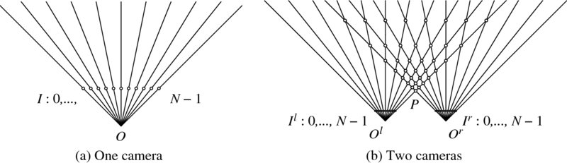
Figure 6.11 Discrete space observed by a camera (a) and two cameras (b)
If two cameras are introduced, as shown in Figure 6.11(b), the observable space becomes even smaller because the space consists of the set of intersecting points of the two rays. Now, only the discrete points on a ray are observable and thus the observable space is a discrete cone. The point, P, indicates the nearest position, where the disparity is maximal, Dmax = N − 1. The point at infinity, that is the vanishing point, is where the parallel rays meet ultimately. In between the two extreme points, iso-disparity lines are formed, where the points are located in the same distance from the optical center.
The key point in this observation is that the observable space is a triangle region (or cone) which consists of intersecting points. From Figure 6.11(b), the observable space is extracted, rescaled, and illustrated in Figure 6.12. Represented on the left is the disparity level, which is equally spaced for convenience. The pixels are located along the horizontal line. The importance of this representation is that the stereo matching can be reduced to a search problem in a discrete triangular region.
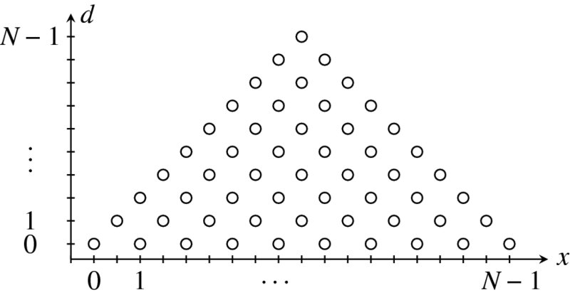
Figure 6.12 The observable space is a discrete triangle. The point at infinity is mapped to the zero disparity
In a trinocular stereo vision system, a third camera is introduced between the two cameras (An et al. 2004; Ueshiba 2006). Being rectified, all the three optical axis are parallel and all the three image planes are coplanar as shown in Figure 6.13. In general, more than one camera system is called multiple view system and described by multiple view geometry (Faugeras and Luong 2004; Hartley and Zisserman 2004). In a multiple view synthesis system, the extra positions between the left and right cameras are considered as positions for virtual images (Karsten et al. 2009; Scharstein 1999; Tian et al. 2009). In a binocular vision system, the intermediate position can be considered as a new coordinate to represent the left and right disparities.
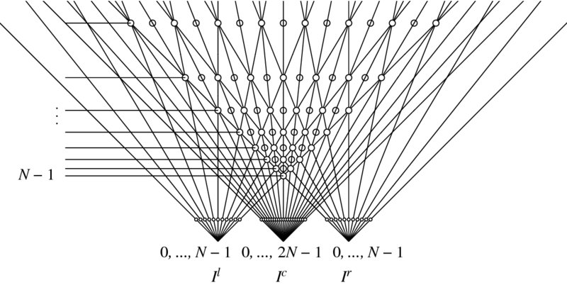
Figure 6.13 Coordinate systems: left (ol), right (or) and center reference (oc)
Let's represent the the new coordinates by oc. The advantage of the new coordinates is that the left and right disparities can be represented in the same coordinates, as a cyclopean view (Julesz 1971; Wolfe et al. 2006). A complete description of disparity needs two quantities (dl, dr). However, this description is possible with a single view, oc. Besides the convenience of representation, the new coordinates let us observe the occluding points. The filled circles are visible commonly by the three coordinates systems. In the left or right system, only one point along the ray is observable. Other points behind the observed point are occluded. However, in the new coordinates, all such occluding points are also visible. The places with empty circles are unobservable by any of the cameras but useful to represent the virtual positions. However, the new representation needs higher resolution than the image: xc ∈ [0, 2N − 1].
The whole effort for coordinates system is to describe the disparity as a function. As disparity is involved with more than one images, reference coordinates are not unique. For binocular stereo, the disparity is represented either by dl or dr. Having introduced a third coordinate, the disparity can be represented by dc. Let the three coordinates be left (reference) coordinates, right (reference) coordinates, and center (reference) coordinates (aka cyclopean coordinates (Belhumeur 1996; Marr and Poggio 1979)). As the number of cameras is increased, the search space becomes sparser but keeps its triangular shape.
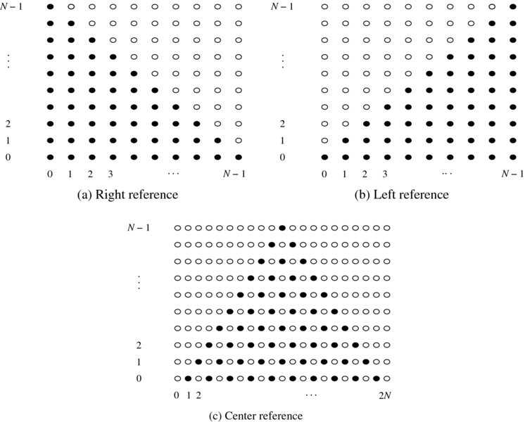
Figure 6.14 Search spaces for disparity (horizontal: pixel and vertical: disparity)
Now, let us examine the search spaces, represented in the three coordinates systems, in terms of disparity computation (Figure 6.14). In the search spaces, the nodes are represented by {(xr, dr)|xr ∈ [0, N − 1], dr ∈ [0, N − 1]}, {(xl, dl)|xl ∈ [0, N − 1], dl ∈ [0, N − 1]}, and {(xc, dc)|xc ∈ [0, 2N − 1], dc ∈ [0, N − 1]}. At first observation, the node types are not all the same, classified as matching, occluding, and virtual. As the name represents, the matching nodes, as denoted by the filled circles, are the places that one or two cameras can observe. Likewise, the occluding nodes, as represented by the empty circles in the left and right systems, are the places which cannot be observed by two cameras simultaneously. The empty nodes in the center reference system, the so-called virtual nodes, are different from the occluding nodes, because they are introduced to fill the spaces in a regular manner.
In the second observation, the search space is characterized by triangular distribution of matching nodes. This means that, for the right disparity, the number of candidate matching points becomes less as we move to the right boundary. The reverse is true for the left disparity. For the center reference, the uncertainty increases at both ends. This property naturally affects the disparity map, with blurred values around image boundaries.
The legal disparity is interpreted here as a connected path from one side to the other side, which represents the dissection of the object surface in some transformed way. Assigning penalties and constraints on the possible paths, the stereo matching becomes the shortest paths problem. For the left and right systems, the path should be positioned in the matching nodes area, because the occluding region is unobserved. However, in the center reference system, the shortest path may pass through the empty nodes, because they are not actually occluding points but virtual points, to make the search path smooth if required.
Choosing matching nodes must be based on observations, Il and Ir as well as the smoothness between neighbor nodes. Analogously, choosing virtual nodes must be based on some prior, such as smoothness constraints. The appearance model and the geometric constraints play roles in defining good paths in these spaces.
Since the the three coordinates represent the same scene, there exist relationships between the coordinates systems. Suppose that (xl, xr, xc) are the corresponding points with the disparities, (dl, dr, dc). Then, the center disparity and the corresponding points are related as follows:
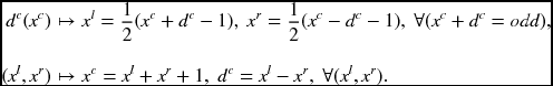
First, if xc + dc = odd, the disparity dc(xc) specifies the conjugate pair, ![]() . For i + dc = even, the node has no corresponding image pixels. Second, the conjugate pair, (Il(xl), Ir(xr)), specifies the disparity, dc(xl + xr + 1) = xl − xr.
. For i + dc = even, the node has no corresponding image pixels. Second, the conjugate pair, (Il(xl), Ir(xr)), specifies the disparity, dc(xl + xr + 1) = xl − xr.
Similarly, the left and right disparities have the following relationships.
By these equations, disparities in one coordinates system can be transformed into another coordinate system. Moreover, the equations naturally represent the geometric constraints of the disparities and corresponding points in stereo matching. Assuming multiple views and discrete observations, we obtain a lot of constraints that must be satisfied by the legal disparities.
6.12 Constraints in Frequency Space
So far we have studied disparity as a warping function in the space domain. The notion of spatial warping can be expanded to the spectral domain, regarded as a phase warping in the spectral domain (Candocia and Adjouadi 1997; Fookes et al. 2004; Lucey et al. 2013; Sheu and Wu 1995). This view can be expanded to the space-time space, often called the space-time cube, and frequency representation of both space and time.
As a similar vision module, motion is known to have a certain conservation law in the frequency domain (Fleet and Jepson 1990, 1993; Gautama and van Hulle 2002). However, the same is not true in stereo vision. The major reason is that the optical flows can be modeled as differentials but the disparity cannot be modeled in that way. Any linear approximation of the photometric conservation laws is over-simplification. Nevertheless, the disparity, as a warping function, has certain properties in the spectral domain.
Let's consider two line images g(x) and h(x), and a disparity function, ϕ(x) = x + d(x). Then, the target function can be regarded as a composite function: h(x) = g(ϕ(x)). The goal of stereo matching is interpreted as finding the warping function for the given g( · ) and h( · ). In this case, the reference coordinates is the left image and thus the left disparity is obtained. Changing the role of the two images, we can obtain the other type of disparity, the right disparity.
To proceed further, let's first investigate the properties of the warping function in the spectral domain. In discrete space, the functions are represented by vectors.
Let G and H be the DFTs s of g and h, respectively. Then, the image vectors have the forms:
where W is the DFT matrix:
Then, the composite function, h(x), can be represented as
Taking the DFT of h(x), we have
Next, let us switch the order of integration. Then, we get
Noticing that the inner integral is independent of G, we give it its own name, P(k, l) (Bergner et al. 2006),
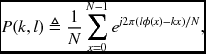
and call it the spectral warping function (SWF). Substituting Equation (6.88) into (6.87) yields
In vector notation, this equation becomes
where P = {pk, l}.
Now, all the important properties of the disparity are included in SWF. Note that P(k, l) is point-symmetric:
The kernel P is independent of the properties of g and solely depends on ϕ. Also, it can be interpreted as a map telling how a certain frequency component of G is mapped to a frequency in the target spectrum of H.
Figure 6.15 depicts intensity and warping functions and their spectral warping matrix P(k, l) for the test stereo dataset. The graphs on the second row contain the intensity function f(x) of the reference frame and the warping function ϕ(x) along the indicated scan line, respectively. The plot in the last row shows profiles of the corresponding kernel maps. Equation (6.90) means that G(l) is integrated along the column k of the kernel map to produce H(k). If the warping is constant, the kernel map is also uniform. Otherwise, the input spectrum is modulated by the kernel to produce the resulting spectrum.
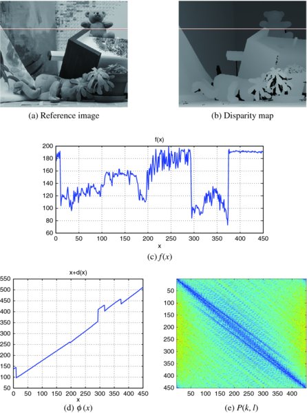
Figure 6.15 Profile, disparity, and SWP for the scan line
The spectral warping function can be factorized further. Consider the N × N matrices:
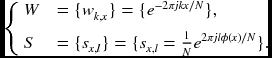
Then, Equation (6.88) becomes
Because of this, Equation (6.90) is decomposed into the factorization:
In this expression, the disparity is decomposed into the position and value, represented by the two phasor matrices, W and S. The two phasors are the unit vectors positioned in a unit circle. The constraints for the disparity appear as the phasor magnitude and ordering in the spectral domain.
The matrix S is orthogonal:
though it is not unitary due to the asymmetric definition of DFT. Containing the disparity as phasor, S is the variable to be recovered. In the spectrum, information on disparity is encoded in the phasor position and their order. Like angle modulation, the noise on disparity tends to affect the phasor amplitude rather than its phase. (See the problems at the end of this chapter.)
6.13 Basic Energy Functions
We have observed that the central problem of depth estimation is the stereo matching that searches for an optimal disparity. The major mechanism for disparity is the photometric constraint, Equation (6.71), which defines the brightness invariance between a pair of corresponding points. However, the disparity cannot be determined uniquely because it is not one-to-one mapping. To narrow down the vast search space, various constraints are introduced.
In the energy representation, the photometric constraint plays a major role and the other constraints play a role of limiting the search space.
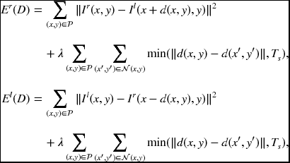
where λ is the Lagrange multiplier and Ts is the threshold. The first term comes from the photometric constraint, Equation (6.71), and is defined along the epipolar line. The second term comes from the smoothness constraint, Equation (6.72), and is defined over local neighborhood. The parameter, λ, is a Lagrange multiplier, which makes the problem unconstrained minimization. To detect the occlusion, both the left and right disparities must be obtained, as discussed in Equation (6.74).
There is a third viewpoint, the center referenced system, where the energy function can be defined, with the help of Equation (6.80),
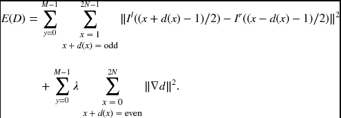
Note that xc ∈ [0, 2N], while xl, xr ∈ [0, N − 1], due to Equations (6.80) and (6.81).
Although defined on the image plane, the energy function can be alternatively defined for an epipolar line. The DP algorithm can manage one line at a time but other algorithms, such as relaxation, BP, and GC, can manage globally the entire image plane or part of it.
Equations (6.96) and (6.97) are the most basic forms of stereo matching. Various alternative representations may be derived by combining appearance and geometric constraints, features, and measures. The additional constraints may be directional smoothness and occlusion indicator which turns and off the smoothness term. Unless otherwise stated, these basic forms will be used as baseline equations for circuit design, though some modifications may be inevitable.
Problems
- 6.1 [Correspondence] Using Equation (6.45), show that the epipolar line is collinear and that the corresponding points are located on it.
- 6.2 [Correspondence] Derive ET = [el]×H− 1 in Equation (6.41).
- 6.3 [Correspondence] For parallel optics, derive the essential matrix. Check for the essential matrix equation.
- 6.4 [Correspondence] For parallel cameras, derive the fundamental matrix and check for the fundamental matrix equation. What is the epipole?
- 6.5 [Correspondence] What does the fundamental matrix mean in the rectified system?
- 6.6 [Rectification] In Equation (6.62), derive the three component of Rrect. Check for the parallel camera system.
- 6.7 [Rectification] Consider a rectified system. In reference to the world coordinates, the cameras are located at ( − B/2, 0, 0)T and (B/2, 0, 0)T and the principal points are defined at ( − B/2, 0, f)T and (B/2, 0, f)T, where f is the focal length and B is the baseline between the two camera centers. If the disparity is defined as d = xl − xr, what is the position of the object, (X, Y, Z)?
- 6.8 [Rectification] Repeat the previous problem, when the world coordinates coincide with the left camera and the right camera.
- 6.9 [Rectification] For the rectified system, with baseline B and focal length f, derive the camera and fundamental matrices.
- 6.10 [Spectrum] Solve Equation (6.94) for S using pseudo-inverse and discuss the properties.
References
- An L, Jia Y, Wang J, Zhang X, and Li M 2004 An efficient rectification method for trinocular stereovision. Pattern Recognition, 2004. ICPR 2004. Proceedings of the 17th International Conference on, vol. 4, pp. 56–59 IEEE.
- Belhumeur PN 1996 A Bayesian approach to binocular steropsis. International Journal of Computer Vision 19(3), 237–260.
- Bergner S, Muler T, Weiskopf D, and Muraki D 2006 A spectral analysis of function composition and its implications for sampling in direct volume visualization. IEEE Trans. Vis. Comput. Graph. 12(5), 1353–1360.
- Bleyer M and Gelautz M 2007 Graph-cut-based stereo matching using image segmentation with symmetrical treatment of occlusions. Signal Processing: Image Communication 22(2), 127–143.
- Bleyer M, Rother C, and Kohli P 2010 Surface stereo with soft segmentation. Computer Vision and Pattern Recognition (CVPR), 2010 IEEE Conference on, pp. 1570–1577 IEEE.
- Brahmachari AS and Sarkar S 2013 Hop-diffusion Monte Carlo for epipolar geometry estimation between very wide-baseline images. IEEE Trans. Pattern Anal. Mach. Intell. 35(3), 755–762.
- Candocia F and Adjouadi M 1997 A similarity measure for stereo feature matching. IEEE Trans. Image Processing 6(10), 1460–1464.
- Chin TJ, Wang H, and Suter D 2009 Robust fitting of multiple structures: The statistical learning approach. ICCV, pp. 413–420 IEEE.
- Chojnacki W and Brooks MJ 2007 On the consistency of the normalized eight-point algorithm. Journal of Mathematical Imaging and Vision 28(1), 19–27.
- de Villiers JP, Leuschner FW, and Geldenhuys R 2010 Modeling of radial asymmetry in lens distortion facilitated by modern optimization techniques. IS&T/SPIE Electronic Imaging, pp. 75390J–75390J International Society for Optics and Photonics.
- Deng Y, Yang Q, Lin X, and Tang X 2005 A symmetric patch-based correspondence model for occlusion handling. Computer Vision, 2005. ICCV 2005. Tenth IEEE International Conference on, vol. 2, pp. 1316–1322 IEEE.
- Dubrofsky E 2007 Homography estimation Master's thesis Carleton University.
- Faugeras O 1993 Three-Dimensional Computer Vision: A Geometric Viewpoint. MIT Press, Cambridge, Massachusetts.
- Faugeras O and Luong Q 2004 The Geometry of Multiple Images: The Laws That Govern the Formation of Multiple Images of a Scene and Some of Their Applications. MIT Press.
- Faugeras O, Luong Q, and Maybank S 1992 Camera self-calibration: Theory and experiments. ECCV, pp. 321–334.
- Fleet DJ and Jepson AD 1990 Computation of component image velocity from local phase information. International Journal of Computer Vision 5(1), 77–104.
- Fleet DJ and Jepson AD 1993 Stability of phase information. IEEE Trans. Pattern Anal. Mach. Intell. 15(12), 1253–1268.
- Fookes C, Maeder A, Sridharan S, and Cook J 2004 Multi-spectral stereo image matching using mutual information. 3D Data Processing, Visualization and Transmission, 2004. 3DPVT . Proceedings. 2nd International Symposium on, pp. 961–968 IEEE.
- Forsyth D and Ponce J 2003 Computer Vision: A Modern Approach. Prentice Hall.
- Fusiello A, Trucco E, and Verri A 2000 A compact algorithm for rectification of stereo pairs. Machine Vision Application 12(1), 16–22.
- Gautama T and van Hulle MM 2002 A phase-based approach to the estimation of the optical flow field using spatial filtering. IEEE Trans. Neural Networks 13(5), 1127–1136.
- Hartley R and Li H 2012 An efficient hidden variable approach to minimal-case camera motion estimation. IEEE Trans. Pattern Anal. Mach. Intell. 34(12), 2303–2314.
- Hartley R and Zisserman A 2004 Multiple View Geometry in Computer Vision. Cambridge University Press.
- Hartley RI 1997 In defense of the eight-point algorithm. IEEE Trans. Pattern Anal. Mach. Intell. 19(6), 580–593.
- Hong L and Chen GQ 2008 Segment based image matching method and system. US Patent 7,330,593.
- Julesz B 1971 Foundations of Cyclopean Perception. University of Chicago Press.
- Kang YS and Ho YS 2011 An efficient image rectification method for parallel multi-camera arrangement. Consumer Electronics, IEEE Transactions on 57(3), 1041–1048.
- Karsten M, Aljoscha S, Kristina D, Philipp M, Peter K, Thomas W et al. 2009 View synthesis for advanced 3D video systems. EURASIP Journal on Image and Video Processing 2008, 1–11.
- Kolmogorov V 2005 Graph Cut Algorithms for Binocular Stereo with Occlusions. Springer-Verlag.
- Lin MH and Tomasi C 2003 Surfaces with occlusions from layered stereo. Computer Vision and Pattern Recognition, 2003. Proceedings. 2003 IEEE Computer Society Conference on, vol. 1, pp. I–710 IEEE.
- Longuet-Higgins HC 1981 A computer algorithm for reconstructing a scene from two projections. Nature 293(5828), 133–135.
- Loop C and Zhang Z 1999 Computing rectifying homographies for stereo vision. Computer Vision and Pattern Recognition, 1999. IEEE Computer Society Conference on., vol. 1 IEEE.
- Lucey S, Ashrat RNN, and Sridharan S 2013 Fourier Lukas-Kanade algorithm. IEEE Trans. Pattern Anal. Mach. Intell. 35(6), 1383–1396.
- Luong Q and Faugeras O 1996 The fundamental matrix: Theory, algorithms, and stability analysis. International Journal of Computer Vision 17(1), 43–75.
- Marr D and Poggio T 1979 A computational theory of human stereo vision. jChemPhys 21(6), 1087–1092.
- Middlebury U 2013 Middlebury stereo home page http://vision.middlebury.edu/stereo (accessed Sept. 4, 2013).
- Min D and Sohn K 2008 Cost aggregation and occlusion handling with WLS in stereo matching. IEEE Trans. Image Processing 17(8), 1431–1442.
- Miraldo P and Araújo H 2013 Calibration of smooth camera models. IEEE Trans. Pattern Anal. Mach. Intell. 35(9), 2091–2103.
- Ni K, Jin H, and Dellaert F 2009 Groupsac: Efficient consensus in the presence of groupings. ICCV, pp. 2193–2200. IEEE.
- Ogale AS and Aloimonos Y 2004 Stereo correspondence with slanted surfaces: Critical implications of horizontal slant. Computer Vision and Pattern Recognition, 2004. CVPR 2004. Proceedings of the 2004 IEEE Computer Society Conference on, vol. 1, pp. I–568 IEEE.
- OpenCV 2013 Camera calibration and 3D reconstruction http://docs.opencv.org/master/modules/calib3d/doc/ -camera_calibration_and_3d_reconstruction.html?highlight=bouguet (accessed Oct. 11, 2013).
- Oram D 2001 Rectification for any epipolar geometry. BMVC, p. Session 7: Geometry and Structure.
- Pollefeys M, Koch R, and Van Gool L 1999 A simple and efficient rectification method for general motion. Computer Vision, 1999. The Proceedings of the Seventh IEEE International Conference on, vol. 1, pp. 496–501 IEEE.
- Rozenfeld S and Shimshoni I 2005 The modified pbM-estimator method and a runtime analysis technique for the RANSAC family. CVPR, pp. I: 1113–1120.
- Scharstein D 1999 View Synthesis using Stereo Vision. Springer-Verlag.
- Scharstein D and Szeliski R 2002 A taxonomy and evaluation of dense two-frame stereo correspondence algorithms. International Journal of Computer Vision 47(1–3), 7–42.
- Sheu HT and Wu MF 1995 Fourier descriptor based technique for reconstructing 3D contours from stereo images. IEE Proceedings-Vision, Image and Signal Processing 142(2), 95–104.
- Sun J, Li Y, Kang SB, and Shum HY 2005 Symmetric stereo matching for occlusion handling. Computer Vision and Pattern Recognition, 2005. CVPR 2005. IEEE Computer Society Conference on, vol. 2, pp. 399–406 IEEE.
- Tao H, Sawhney HS, and Kumar R 2001 A global matching framework for stereo computation. Computer Vision, 2001. ICCV 2001. Proceedings. Eighth IEEE International Conference on, vol. 1, pp. 532–539 IEEE.
- Tian D, Lai PL, Lopez P, and Gomila C 2009 View synthesis techniques for 3D video. SPIE Optical Engineering+ Applications, pp. 74430T–74430T International Society for Optics and Photonics.
- Tippetts BJ, Lee DJ, Lillywhite K and Archibald J 2013 Review of stereo vision algorithms and their suitability for resource-limited systems http://link.springer.com/article/10.1007%2Fs11554-012-0313-2 Sept. 4, 2013).
- Tola E, Lepetit V, and Fua P 2010 Daisy: An efficient dense descriptor applied to wide-baseline stereo. IEEE Trans. Pattern Anal. Mach. Intell. 32(5), 815–830.
- Trucco E and Verri A 1998 Introductory Techniques for 3-D Computer Vision. Prentice Hall.
- Tsai R 1987 A versatile camera calibration technique for high-accuracy 3D machine vision metrology using off-the-shelf tv cameras and lenses. Robotics and Automation, IEEE Journal of 3(4), 323–344.
- Ueshiba T 2006 An efficient implementation technique of bidirectional matching for real-time trinocular stereo vision. Pattern Recognition, 2006. ICPR 2006. 18th International Conference on, vol. 1, pp. 1076–1079 IEEE.
- Weng J, Cohen P, and Herniou M 1992 Camera calibration with distortion models and accuracy evaluation. IEEE Trans. Pattern Anal. Mach. Intell. 14(10), 965–980.
- Wolfe JM, Kluender KR, Levi DM, Bartoshuk LM, Herz RS, Klatzky RL, and Lederman SJ 2006 Sensation & Perception. Sinauer Associates Sunderland, MA.
- Woodford O, Torr P, Reid I, and Fitzgibbon A 2009 Global stereo reconstruction under second-order smoothness priors. IEEE Trans. Pattern Anal. Mach. Intell. 31(12), 2115–2128.
- Yu Y 2012 Estimation of Markov random field parameters using ant colony optimization for continuous domains. 2012 Spring Congress on Engineering and Technology, pp. 1–4.
- Zhang Z 2000 A flexible new technique for camera calibration. IEEE Trans. Pattern Anal. Mach. Intell. 22(11), 1330–1334.
- Zheng Y, Sugimoto S, and Okutomi M 2011 A Branch and Contract algorithm for globally optimal fundamental matrix estimation. CVPR, pp. 2953–2960 IEEE.
- Zitnick CL and Kanade T 2000 A cooperative algorithm for stereo matching and occlusion detection. IEEE Trans. Pattern Anal. Mach. Intell. 22(7), 675–684.
- Zitnick CL, Kang SB, Uyttendaele M, Winder S, and Szeliski R 2004 High-quality video view interpolation using a layered representation. ACM Transactions on Graphics (TOG), vol. 23, pp. 600–608 ACM.