Generalized ANN

At this point in the book, I have covered quite a bit on the subject of ANN, but there is still a considerable amount to discuss. What should be clear to you at this stage in the book is that an ANN is a mathematical representation or model of the many neurons and their interconnections in a human brain. ANN basics were discussed in Chapter 2. I introduced you to a specialized ANN in Chapter 7 that was well suited for a fairly simple robotic application. However, the field of ANNs is quite broad and there is still much to cover.

In this chapter’s title, I used the phrase deep learning, which I also briefly mentioned in Chapter 2. Deep learning is commonly used by AI practitioners to refer to multilayer ANNs, which are able to learn by having repeated training data sets applied to them. Figure 8-1 shows a three-layer ANN.

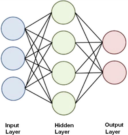
Figure 8-1. Three-layer ANN

The following explains the layers shown in Figure 8-1.

• Input: Inputs are applied to this layer.

• Hidden: All layers that are not classified as input or output are hidden.

• Output: Outputs appear at this layer.

All the neurons or nodes are interconnected to each other, layer by layer. This means that the input layer connects to all the nodes in the first hidden layer. Likewise, all the nodes in the last hidden layer connect to the output nodes.

I have also referred to this network configuration as a generalized ANN to differentiate from the Hopfield network, which is a special case from the general. The Hopfield network only consists of a single layer where all the nodes serve as both inputs and outputs, and there are no hidden layers. From this point on when I speak of an ANN, I am referring to the generalized type with multiple layers.

There are two broad categories for ANNs:

• FeedForward: Data flow is unidirectional. Nodes send data from one layer to the next one.

• Feedback: Data is bidirectional using feedback loops.

Figure 8-2 shows models for both of these ANN types.

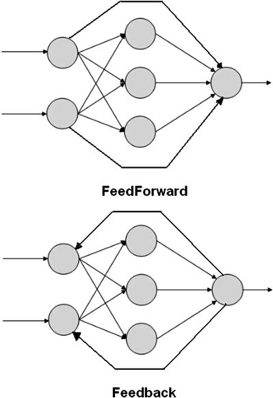
Figure 8-2. FeedForward and Feedback ANN models

An input to an ANN is just a pattern of numbers that propagate through the network where each node sums the inputs and if the sum exceeds a threshold value causes the node to fire and output a number to the next connected node. The connection strength between nodes is known as the weighting, as I have previously described in the Hopfield network. Determining the weight values is the key element in how an ANN learns. ANN learning usually happens when many training data sets are applied to the network. These training data sets contain both input and output data. The input data creates output data, which is then compared to the true output data with error results created when the values do not agree. This error data is consequently feedback through the ANN and the weights adjusted in an incremental fashion in accordance with a pre-programmed learning algorithm. Over many training cycles, often thousands, the ANN is trained to compute the desired output for a given input. This learning technique is called back propagation.

Figure 8-3 shows a three-layer ANN with all the associated weights interconnecting the nodes. The weights are shown in a w_i,j notation where i is the source node and j is the receiving or destination node. The stronger the weight the more the source node affects the destination node. Of course, the reverse is also true.

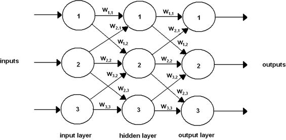
Figure 8-3. Three-layer ANN with weights

If you examine Figure 8-3 closely, you see that not all layer-to-layer nodes are interconnected. For instance, input layer node 1 has no connection with hidden layer node 3. This can be remedied if it is determined that the network cannot be adequately trained. Adding more node-to-node connections is quite easy to do using matrix operations, as you will see shortly. Adding more connections does no real harm because the connection weights are adjusted. The network is trained to the point where unnecessary connections are assigned a 0 weighting value, which effectively removes them from the network.

At this point, it is useful to actually follow a signal path through a simplified ANN so that that you have a good understanding of the inner workings of this type of network. I use a very simple two-layer, four-node network for this example because it more than suffices for this purpose. Figure 8-4 shows this network, which only consists of one input and one output layer. No hidden layers are necessary in this ANN.

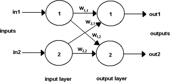
Figure 8-4. Two-layer ANN

Now, let’s assign the following values to the inputs and weights shown in Figure 8-4, as listed in Table 8-1.

These values were selected randomly and do not represent nor model any physical situation. Often times, weights are randomly assigned with the intention that it is easier to promote a rapid convergence to an optimal, trained solution. With so few inputs and weights involved, I did not see it as an issue to omit a diagram with these real values. You can easily scribble out a diagram with the values if that helps you understand the following steps.

I start the calculation with node 1 in layer 2 because there are no modifications that take place between the data input and the input nodes. The input nodes exist as a convenience for network computations. There is no weighting directly applied by the input layer nodes to the data input set. Recall from Chapter 2 that the node sums all the weighted inputs from all of its interconnected nodes. In this case, node 1 in layer 2 has inputs from both nodes in layer 1. The weighted sum is therefore

w_1,1 * in1 + w_2,1 * in2 = 0.8 * 0.8 + 0.9 * 0.4 = 0.64 + 0.36 = 1.00

Let’s next assume that the activation function is the standard sigmoid expression that I also described in Chapter 2. The sigmoid equation is:

where e = math constant 2.71828…

With x = 1.0, this equation becomes:

= 1/(1.3679) = 0.7310 or out1 = 0.7310

Repeating the preceding steps for the other node in layer 2 yields the following:

w_2,2 * in2 + w_1,2 * in1 = 0.4*0.4 + 0.1*0.8 = 0.16 + 0.08 = 0.24

Letting x = 0.24 yields this:

= 1/(1.7866) = 0.5597 or out2 = 0.5597

The two ANN outputs have now been determined for the specific input data set. This was a fair amount of manual calculations to perform for this extremely simple two-layer, four-node ANN. I believe you can easily see that it is nearly impossible to manually perform these calculations on much larger networks without generating errors. That is where the computer excels in performing these tedious calculations without error for large ANNs with many layers. I used numpy matrices in the last chapter when doing the Hopfield network multiplications and dot products. Similar matrix operations are applied to this network. The input vector for this example is just the two values: in1 and in2. They are expressed in a vector format as

Likewise, the following is the weighting matrix:

Figure 8-5 shows these matrix operations being applied in an interactive Python session. Notice that it only takes a few statements to come up with exactly the same results as was done with the manual calculations.

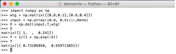
Figure 8-5. Interactive Python session

The next example involves a larger ANN that is handled entirely by a Python script.

Larger ANN

This example involves a three-layer ANN that has three nodes in each layer. The ANN model is shown in Figure 8-6 with an input data set and a portion of the weighting values in an effort not to obscure the diagram.

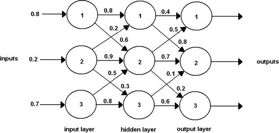
Figure 8-6. Larger ANN

Let’s start with the input data set as that is quite simple. This is shown in a vector format as follows:

There are two weighting matrices in this example. One is needed to represent the weights between the input layer (wtg_ih) and the hidden layer and the other for the weights between the hidden layer and the output layer (wtg_ho). The weights are randomly assigned as was done for the previous examples.

Figure 8-7 shows the matrix multiplication for the input to the hidden layer. The resultant matrix is shown as X1 in the screenshot.

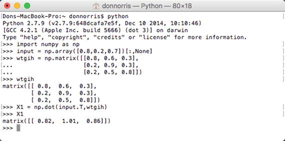
Figure 8-7. First matrix multiplication

The sigmoid activation function has to be applied next to this resultant. I called the transformed matrix O1 to indicate it was an output from the hidden layer to the real output layer. The resultant O1 matrix is:

matrix([[ 0.69423634,  0.73302015,  0.70266065]])

These are the values multiplied by the weighting matrix wtg_ho. Figure 8-8 shows this multiplication. I called the resultant matrix X2 to differentiate from the first one. The final sigmoid calculation is also shown in the screenshot, which I named O2.

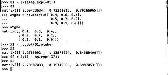
Figure 8-8. Second matrix multiplication

The matrix O2 is also the final output from the ANN, which is

matrix([[ 0.78187033,  0.7574536,  0.69970531]])

This output should reflect the input so let’s compare the two and calculate the error or difference between the two. All of this is shown in Table 8-2.

Table 8-2. Comparison of ANN Outputs with the Inputs

Input	Output	Error
0.8	0.78187033	0.01812967
0.2	0.7574536	-0.5574536
0.7	0.69970531	0.00029469

The results are actually quite remarkable as two of the three outputs are very close to the respective input values. However, the middle value is way off, which indicates that at least some of the ANN weights must be modified. But, how do you do it?

Before I show you how that is done, please consider the situation shown in Figure 8-9.

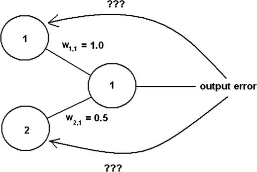
Figure 8-9. Error allocation problem

In Figure 8-9, two nodes are connected to one output node, which has an error value. How can the error be reflected back to the weights interconnecting the nodes? In one case, you could evenly split the error between the input nodes. However, that would not accurately represent the true error contribution from the input nodes as node 1 has twice the weight or impact as node 2. A moments thought should lead you to the correct solution that the error should be divided in direct proportion to the weighting values connecting the nodes. In the case of the two input nodes shown in Figure 8-9, node 1 should be responsible for two-thirds of the error while node 2 should have one-third of the error contribution, which is precisely the ratios of their respective weights to the sum applied to the output node.

This use of the weights in this fashion is an additional feature for the weighting matrix. Normally, weights are applied to signals propagating in a forward direction through the ANN. However, this approach uses weights with the error value, which is then propagated in a backwards direction. This is reason that error determination is also called back propagation.

Consider next what would happen if there were errors appearing at more than one output node, which is likely the case in most initial ANN startups. Figure 8-10 shows this situation.

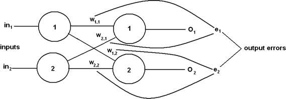
Figure 8-10. Error allocation problem for multiple output nodes

It turns out the process is identical for multiple nodes as it was for a single node. This is true because the output nodes are independent of one another, with no interconnecting links. If this were not true, it would be very difficult to back propagate from interlinked output nodes.

The equation to apportion the error is also very simple. It is a just a fraction based on the weights connected to the output node. For instance, to determine the correction for e₁ in Figure 8-10, the fractions applied to w_1,1 and w_2,1 are as follows:

• w_1,1/( w_1,1 + w_2,1)  and   w_2,1/( w_1,1 + w_2,1)

Similarly, the following are the errors for e₂.

• w_1,2/( w_1,2 + w_2,2)  and   w_2,2/( w_1,2 + w_2,2)

So far, the process to adjust the weights based on the output errors has been quite simple. The errors are easy to determine because the training data provides the correct answers. For two-layer ANNs, this is all that is needed. But how do you handle a three-layer ANN where there are most certainly errors in the hidden layer output, yet there is no training data available, which can be used to determine the error values?

Back Propagation In Three-layer ANNs

Figure 8-11 shows a three-layer, six-node ANN with two nodes per layer. I deliberately simplified this ANN so that it is relatively easy to focus on the limited back propagation required for the network.

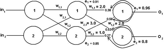
Figure 8-11. Three-layer, six-node ANN with error values

In Figure 8-11, you should be able to see the output error values that were arbitrarily created for this example. Individual error contributions from nodes 1 and 2 of the hidden layer are shown at the inputs to each of the output nodes . These normalized values were calculated as follows:

• e_1output1 * w_1,1/(w_1,1 + w_2,1) = 0.96 * 2/(2 + 3) = 0.96 * 0.4 = 0.38

• e_1output2 * w_2,1/(w_1,1 + w_2,1) = 0.96 * 3/(2 + 3) = 0.96 * 0.6 = 0.58

• e_2output1 * w_1,2/(w_1,2 + w_2,2) = 0.8 * 2/(2 + 1) = 0.8 * 0.66 = 0.53

• e_2output2 * w_2,2/(w_1,2 + w_2,2) = 0.8 * 1/(2 + 1) = 0.8 * 0.33 = 0.27

The total normalized error value for each hidden node is the sum of the individual error contributions to a given output node and are calculated as follows:

• e₁ = e_1output1 + e_2output1 = 0.38 + 0.53 = 0.91

• e₂ = e_1output2 + e_2output2 = 0.58 + 0.27 = 0.85

These values are shown next to each of the hidden nodes in Figure 8-11.

The preceding process may be continued as needed to calculate all the combined error values for any remaining hidden layers. There is no need to calculate error values for the input layer because it must be 0 for all input nodes as they simply pass the input values without any modifications.

The preceding process for calculating the hidden layer error outputs is quite tedious since it was done manually. It would be much nicer if it could be automated using matrices in a similar way that the feed forward calculations were done. The following would result if the matrices were translated on a one-to-one basis from the manual method :

Unfortunately, there is no reasonable way to input the fractions that are shown in the preceding matrix. But all hope is not lost if you think about what the fractions actually do. They normalize the node’s error contribution, meaning that the fraction converts to a number ranging between 0 and 1.0. The relative error contribution can also be expressed as an unnormalized number by simply using the weight numerator and dropping the denominator. The result is still acceptable because it is really only important to calculate a combined error value that is useful in the weight updates. I cover this in the next section.

Removing the denominators of all the fractions yields

The preceding matrix can easily be handled using numpy’s matrix operations. The only catch is that the transpose of the matrix must be used in the multiplication, which again is not an issue. Figure 8-12 shows the actual matrix operations for this error backpropagation example.

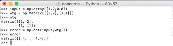
Figure 8-12. Hidden layer error matrix multiplication

It is now time to discuss how the weighting matrix values are updated once the errors have been determined.

Updating the Weighting Matrix

Updating the weighting matrix is the heart of the ANN learning process. The quality of this matrix determines how effective the ANN is in solving its particular AI problem. However, there is a very significant problem in trying to mathematically determine a node’s output given its input and weights. Consider the following equation, which is applicable to a three-layer, nine-node ANN that determines the value appearing at a particular output node:

O _k is the output at the k _th node.

w _j,k is all the interconnecting weights between the input layer and selected output node.

x _i are the input values.

This certainly is a formidable equation even though it only deals with a relatively simple three-layer, nine-node ANN. You can probably imagine the horrendous equation that would model a six-input, five-layer ANN, which in itself is not that large of an ANN. Larger ANN equations are likely beyond human comprehension. So how is this conundrum solved?

You could try a brute-force approach , where a fast computer simply tries a series of different values for each weight. Let’s say there are 1000 values to test for each weight, ranging from –1 to 1 in increments of 0.002. Negative weights are allowed in an ANN and the 0.002 increment is probably fine to determine an accurate weight. However, for our three-layer, nine-node ANN there are 18 possible weighting links. Since there are 1000 values per link, there are 18,000 possibilities to test. That means it would take approximately five hours to go through all the combinations if the computer took one second for each combination. Five hours is not that bad for a simple ANN, however, the elapsed time would grow exponentially for larger ANNs. For example, in a very practical 500-node ANN, there are about 500 million weight combinations. Testing at one second per combination would take approximately 16 years to complete. And that is only for one training set. Imagine the time taken for thousands of training sets. Obviously, there must be a better way than using the brute-force approach.

The solution for this difficult problem comes from the application of a mathematical approach named steepest descent. This approach was first created in 1847 by a French mathematics professor named Augustin Louis Cauchy. He proposed it in a treatise concerning the solution of a system of simultaneous equations. However, a period of more than 120 years elapsed before mathematicians and AI researchers applied it to ANNs. The field of ANN research rapidly developed once this technique became well known and understood.

The technique is also commonly referred to as gradient descent, which I start doing from this point. The underlying mathematics for gradient descent can be a bit confusing and somewhat obscure, especially when it is applied to ANNs. The following sidebar delves into the details of the gradient descent technique in order to provide those interested readers with a brief background on the subject.

Examining the Gradient Descent Technique

Credit goes to Matt Nedrich, who wrote a great blog in early 2014 from which I have based much of this discussion. At the time, Matt was working for Atomic Objects, a software consultancy based in Ann Arbor, MI. You can view the original blog at https://spin.atomicobject.com .

I start by focusing on a close relative named linear regression. This is not the first time I have discussed linear regression . In Chapter 2, I discussed the concept of a linear predictor using mushrooms in the example. The linear predictor was a sloped line with a generalized equation form of

I didn’t mention it at that time, but this equation is often used a “best fit” predictor for x-y scatter plot data, which is the basis for linear regression. Consider Figure 8-13, which is also the starting gif for an automated plot sequence in Matt’s blog.

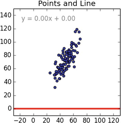
Figure 8-13. Initial x-y scatter plot

The linear regression technique strives to best fit a sloped line that goes through the x-y data points in such a position to minimize the total error if you were to use the sloped line alone as a y predictor for a given x. I recommend going to the blog and clicking on the gif to see the automated sequence as the line seeks a best-fit position. I can only proceed in this book with the mathematical steps that determine the sloped line’s position.

There should be starting equation to kick off this linear regression technique discussion. In this case, it is the sloped line equation used in the Chapter 2 linear predictor model.

where m = slope or gradient

b = y-axis intercept

The general approach is to use a data set of (m, b) and then determine how well that line with those parameters “fits” the x-y data points. This fit is determined by calculating y for a given x in the data set and then calculating the error using the true y in the data set. All the x’s in the data set are used. This error is often referred to as the distance from the sloped line as it makes its way through the data set. This error or distance is also squared to ensure that distances below the line that are negative do not cancel out the positive distances above the line. Squaring the distances also ensures that the overall error function can be differentiated.

The following is a Python method that implements this error function:

# y = mx + b
# m is slope, b is y-intercept
def computeErrorForLineGivenPoints(b, m, points):
    totalError = 0
    for i in range(0, len(points)):
        totalError += (points[i].y - (m * points[i].x + b)) ** 2
    return totalError / float(len(points))

The following is a formal error function for the code implements:

A sloped line generates the best fit when the error—as calculated by the preceding error function—is at its lowest minimum value possible for the totality of the data set. The trick now is to create some form for the error function that provides the appropriate values for m and b that produce the overall minimum. Before I go into that, it would helpful to visualize the relationships between m, b, and e _{m, b} . Figure 8-14 is from the blog that clearly shows the curved nature of the relationships between all the variables.

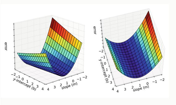
Figure 8-14. Plots form , b and e _m,b

It might also be helpful to imagine holding a marble high up on one of surfaces and allowing it to roll down the slope. It should just stop at the minimum point, which has an m and b associated with it as well as the minimum e _m,b .

Running a gradient descent search is equivalent to rolling the mythical marble down the slope. The first step in doing a gradient descent calculation is to perform two partial differentiations on the error function because it has two independent variables: m and b.

I would like to discuss the concept of a global minimum before I describe the process of calculating the optimum m and b values. Figure 8-15 is a three-dimensional (3D) plot of an analytic continuous function with variables x and y.

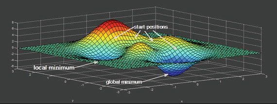
Figure 8-15. Multiple minima 3D plot

In this 3D plot, you can see where two minima or valleys have been identified. One is “deeper” than the other is. The deepest minimum is considered the global minimum, while the other is called a local minimum. Depending upon where you start the gradient descent, it is possible to land in a local minimum while also believing it is the global minimum. Unfortunately, computers do not have the inherent ability to look at 3D image such as Figure 8-15 and figure out where to start the gradient descent to find the true global minimum. It is therefore important to iterate over the entire ranges of the independent variables m and b, taking sufficiently small steps to locate the global minimum and rejecting all local minima. Shortly, you see that setting step size becomes an important part of the process.

All the parts necessary to start the gradient descent have now been discussed. The actual search starts by setting m = –1 and b = 0. This point may be called the origin as a simple reference. The gradient descent should begin its march downhill based on the initial error function towards the optimum solution. Each iteration should also provide an improved solution until it reaches a point where the error remains constant or starts increasing. The direction that an iteration takes is based on the two partial derivatives that were shown earlier.

The following Python code implements this gradient descent algorithm :

def stepGradient(b_current, m_current, points, learningRate):
    b_gradient = 0
    m_gradient = 0
    N = float(len(points))
    for i in range(0, len(points)):
        b_gradient += -(2/N) * (points[i].y - ((m_current*points[i].x) + b_current))
        m_gradient += -(2/N) * points[i].x * (points[i].y - ((m_current * points[i].x) + b_current))                                                                              
    new_b = b_current - (learningRate * b_gradient)
    new_m = m_current - (learningRate * m_gradient)
    return [new_b, new_m]

The learningRate variable controls the step size in the effort to locate the minimum. Too large a step size and you may miss the minimum. However, too small a step size needlessly increases the number of iterations taken before locating the minimum.

Executing the algorithm begins at the origin stated earlier. For each iteration, the m and b values are updated to yield a slightly lower error than the previous iteration. In Figure 18-16, the dot on the left plot displays the current location of the gradient descent search . The right plot displays the corresponding line of best fit for the current m and b values.

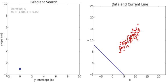
Figure 18-16. Start of the gradient descent

You can clearly see from the right plot that the initial guess for the line of best fit was way off. The fit vastly improves in the next iteration, as shown in Figure 18-17. The left plot now has line indicating the path taken to get there from the initial point.

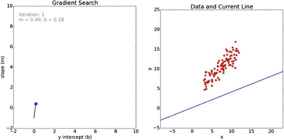
Figure 18-17. Iteration 1 for the gradient search

The fit continues to improve after the next iteration, as shown in Figure 18-18.

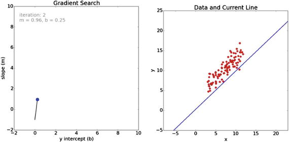
Figure 18-18. Iteration 2 for the gradient search

Finally, after 100 iterations, the search resolves to a very good fit, as shown in Figure 18-19.

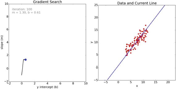
Figure 18-19. Iteration 100 for the gradient search

You can see from the path displayed in the left graph that the search in the last series of iterations took a slight jog downward and to the right in search of the global minimum.

Figure 18-20 is a plot of error values for the first 100 iterations in the gradient search.

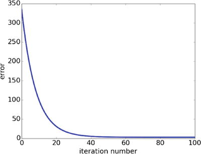
Figure 18-20. Plot of error values vs iteration number

It is good to check on the proper operation of the gradient search. Make sure that the error values continually decrease as the number of iterations increase. Looking at the chart it appears the error values are very close to zero after the 50th iteration. This might well indicate a broad minimum surface exists where the values of m and b would not change significantly in producing a line of best fit.

This is the final line of best fit using 100 iterations in the gradient search:

I hope that you have gained some insight into how the gradient search technique works.

The Gradient Descent Applied to an ANN

Figure 8-21 nicely summarizes the gradient descent technique as it applies to an ANN. It must determine the global minimum by adjusting the weights w_i,j so as to minimize the overall errors present in the ANN.

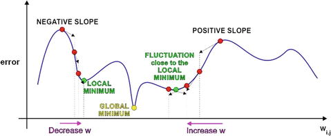
Figure 8-21. ANN global minimum

This adjustment becomes a function of the partial derivative of the error function with respect to a weight, w_j,k. This partial derivative is shown by these symbols: . This derivative is also the slope of the error function. It is the gradient descent algorithm that follows the slope down to the global minimum.

Figure 8-22 shows the three-layer, six-node ANN that is the basis network for the following discussion. Note the i, j, and k indices because they are important to follow as you go through the procedure.

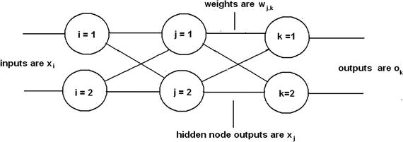
Figure 8-22. Three-layer, six-node ANN

There is one additional symbol required beyond those shown in Figure 8-22: the output node error, which is expressed as

t _k is the true or target value from the training set.

o _k is output resulting from the training set input x _i values.

The total error at any given node n is the preceding equation with n substituted for k. Consequently, the total error for the entire ANN is the sum of all errors for all of the individual nodes. The errors are also squared for reasons mentioned in the sidebar. This leads to the following equation for the error function :

N is the total number of nodes in the ANN.

This error function is the exact one that is required to differentiate with respect to w _j,k  , leading to the following form:

This equation may be considerably simplified by taking note that the error at any specific node is due solely to its input connections. This means the output for the k _th node only depends on the w _j,k weights on its input connections. What this realization does is to remove the summation from the error function because no other nodes contribute to the k _th node’s output. This yields a much simpler error function :

The next step is to do the actual partial differentiation on the function. I simply go through the steps with minimal comments to get to the final equation without prolonging this whole derivation .

1. Chain rule applied:

2. o_k is independent of w_j,k. The first partial =

3. The output o_k has a sigmoid function applied. The second partial = sigmoid

4. The differential of the sigmoid is

5. Combining: . Note the last term is necessary because of the summation term in the sigmoid function. Just another application of the chain rule.

6. Simplifying:

Take a breath, which I often did after a rigorous calculus session. This is the final equation that is used to adjust the weights:

You should also notice that the 2 at the beginning of the equation has been dropped. It was only a scaling factor and not important in determining the direction of the error function slope, which is the main key to the gradient descent algorithm. I do wish to congratulate my readers who have made it this far. Many folks have a very difficult time with the mathematics required to get to this stage.

It would now be very helpful to put a physical interpretation on this complex equation. The first part is just the error, which is easy to see. The sum expressions inside the sigmoid functions are the inputs into the k _th final layer node. And the very last term o _j is the output from the j _th node in the hidden layer. Knowing this physical interpretation should make the creation of the other layer-to-layer error slope expressions much easier.

I state the input to hidden layer error slope equation without subjecting you to the rigorous mathematical derivation. This expression relies on the physical interpretation just presented.

The next step is to demonstrate how new weights are calculated using the preceding error slope expressions . It is actually quite simple as shown in the following equation:

α= learning rate

Yes, that is exactly the same learning rate discussed in Chapter 2 where I introduced it as part of the linear predictor discussion. The learning rate is important because setting it too high may cause the gradient descent to miss the minimum, and setting it too low would cause many extra iterations and lessen the efficiency of the gradient descent algorithm.

Worked-through Example

It’s important to go through a manual example before showing the Python approach, so that you truly understand the process when you run it as a Python script. Figure 8-23 is a slightly modified version of Figure 8-11, on which I have inserted arbitrary hidden node output values to have sufficient data to complete the example.

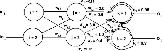
Figure 8-23. Example ANN used for manual calculations

Let’s start by updating w _1,1, which is the weight-connecting node 1 in the hidden layer to node 1 in the output layer. Currently, it has a value of 2.0. This is the error slope equation used for these layer links:

Substitute the values, as shown in the following figure yields:

= e₁ = 0.96

= (2.0 * 0.6) + (3.0 * 0.4) = 2.4

sigmoid = = 0.9168

1 – sigmoid = 0.0832

o ₁= 0.6

Multiply the applicable values with the negative sign yields:

• –0.96 * 0.9168 * 0.0832 * 0.6 = –0.04394

Let’s assume a learning rate of 0.15, which is not too aggressive and the following is the new weight:

• 2.0 – 0.15 * (–0.04394) = 2.0 + 0.0066 = 2.0066

This is not a large change from the original but you must keep in mind that there is hundreds, if not thousands of iterations performed before the global minimum is reached. Small changes rapidly accumulate to some rather large changes in the weights.

The other weights in the network can be adjusted in the same manner as demonstrated.

There are some important issues regarding how well an ANN can learn, which I discuss next.

Issues with ANN Learning

You should realize that not all ANNs learn well, just as not all people learn the same way. Fortunately for ANNs, it has nothing to do with intelligence but rather for more mundane items directly related to the sigmoid activation function. Figure 8-24 is a modified version of Figure 2-12 showing the input and output ranges for the sigmoid function .

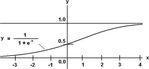
Figure 8-24. Annotated sigmoid function

Looking at Figure 8-24, you should see that if the x inputs are larger than 2.5, the y output has very small changes. This is because the sigmoid function asymptotically approaches 1.0 around that x value. Small changes for large input changes imply very small gradient changes happen. ANN learning becomes suppressed in this situation because the gradient descent algorithm depends upon a reasonable slope being present. Thus, ANN training sets should limit the input x values to what might be called a pseudo-linear range of roughly –3 to 3. Values of x outside this range causes a saturation effect for ANN learning, and no effective weight updates happen.

In a similar fashion, the sigmoid function cannot output values greater than one or less than zero. Output values in those ranges are not possible and weights must be appropriately scaled back such that the allowable output range is always maintained. In reality, the output range should be 0.01 to 0.99 because of the asymptotic nature described earlier.

Initial Weight Selection

Based on the issues just discussed, I believe you can probably realize that it is very important to select a good initial set of ANN weights so that learning can take effect without bumping into input saturation or output limit problems. The obvious choice is to constrain weight selection to the pseudo-linear range I mentioned earlier (i.e., ±3). Often, weights are further constrained to ±1 to be a bit more conservative.

There has been a “rule of thumb” developed over the years by AI researchers and mathematicians that roughly states:

The weights should be initially allocated using a normal distribution set at a mean value equal to the inverse of the square root of the number of nodes in the ANN.

For a 36-node, three-layer ANN, which I have previously used, the mean is or 0.16667. Figure 8-25 shows a normal probability distribution with this mean and ±2 approximate standard deviations are also clearly indicated.

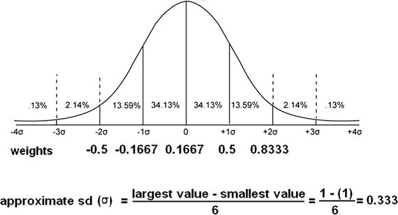
Figure 8-25. Normal distribution of initial weights for a 36-node ANN

A random selection of weights in the range of approximately –0.5 to 0.8333 would nicely provide an excellent starting point for ANN learning for a 36-node network.

Finally, you should avoid setting all weights to the same value because ANN learning depends upon an unequal weight distribution. And obviously, do not set all the weights to 0 because that completely disables the ANN.

This last section completes all of my background discussion on ANN. It is finally time to generate a full-fledged ANN on the Raspberry Pi using Python.

Demo 8-1: ANN Python Scripts

This first demonstration shows you how to create an untrained ANN using Python . I start by discussing the modules that constitute the ANN. Once I have done that, all the modules put into an operative package and the script run. The first module to discuss is the one that creates and initializes the ANN.

def __init__ (self, inode, hnode, onode, lr):
    # Set local variables
    self.inode = inode
    self.hnode = hnode
    self.onode = onode
    self.lr = lr

self.wtgih = np.random.normal(0.1667, 0.3333, self.hnodes, self.inodes)

>>>import numpy as np
>>>wtgih = np.random.normal(0.1667, 0.3333, [3, 3])
>>>wtgih
array([[ 0.44602141,  0.58021837,  0.00499487],
       [ 0.40433922, -0.31695922, -0.40410581],
       [ 0.63401073, -0.37218566,  0.14726115]])

def __init__ (self, inode, hnode, onode, lr):
    # Set local variables
    self.inode = inode
    self.hnode = hnode
    self.onode = onode
    self.lr = lr

    # mean is the reciprocal of the sq root total nodes
    mean = 1/(pow((inode + hnode + onode), 0.5)

    # standard deviation (sd) is approximately 1/6 total weight range
    # total range = 2
    sd = 0.3333

    # generate both weighting matrices
    # input to hidden layer matrix
    self.wtgih = np.random.normal(mean, sd, (hnode, inode])

    # hidden to output layer matrix
    self.wtgho = np.random.normal(mean, sd, [onode, hnode])

def testNet(self, input):
    # convert input tuple to an array
    input = np.array(input, ndmin=2).T

    # multiply input by wtgih
    hInput = np.dot(self.wtgih, input)

    # sigmoid adjustment
    hOutput = 1/(1 + np.exp(-hInput))

    # multiply hidden layer output by wtgho
    oInput = np.dot(self.wtgho, hOutput)

    # sigmoid adjustment
    oOutput = 1/(1 + np.exp(-oInput))

    return oOutput

Test Run

Figure 8-26 shows an interactive Python session that I ran on a Raspberry Pi 3 to test this preliminary code.

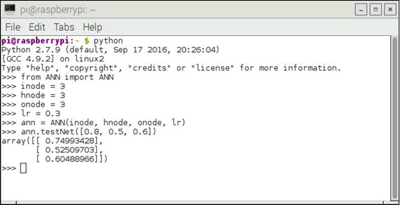
Figure 8-26. Interactive Python session

The init and testNet modules were both part of a class named ANN, which in turn were in a file named ANN.py. I first started Python and imported the class from the file so that the interpreter would recognize the class name. I next instantiated an object named ann with all nodes set to 3 and a learning rate equal to 0.3. The learning rate is not needed yet, but it must be present or you cannot instantiate an object. The act of instantiating an object automatically causes the init module to run. It is expecting size values for all three nodes and a learning rate value.

I next ran the testNet module with the three input values. These are shown in Table 8-4 along with the respective calculated output values. I also included the manually calculated error values.

Table 8-4. Initial Test

Input	Output	Error	Percent error
0.8	0.74993428	–0.05006572	6.3
0.5	0.52509703	0.02509703	5.0
0.6	0.60488966	0.00488966	0.8

The errors are not too much considering this is a totally untrained ANN. The next section discusses how to train an ANN to greatly improve its accuracy.

Demo 8-2: Training an ANN

In this demonstration, I show you how to train an ANN using a third module named trainNet, which has been added to the ANN class definition. This module functions in a very similar fashion to the testNet function by calculating an output set based on an input data set. However, the trainNet module input data is a predetermined training set instead of an arbitrary data tuple as I just demonstrated. This new module also calculates an error set by comparing the ANN outputs with its inputs and using the differences for training the network. The outputs are calculated in exactly the same manner as was done in testNet module. The arguments to trainNet now include both an input list and a training list. The following statements create these arrays from the list arguments:

def trainNet(self, inputT, train):
    # This module depends on the values, arrays and matrices
    # created when the init module is run.

    # create the arrays from the list arguments
    self.inputT = np.array(inputT, ndmin=2).T
    self.train = np.array(train, ndmin=2).T

The error is as stated before is the difference between the training set outputs and the actual outputs. The error equation for the k _th output node as previously stated is:

The matrix notation for the output errors is

self.eOutput = self.train - self.oOutput

The hidden layer error array in matrix notation for this example ANN is

The following is the Python statement to generate this array:

self.hError = np.dot(self.wtgho.T, self.eOutput)

The following is the update equation for adjusting a link between the j _th and k _th layers, as previously shown:

The new gd(w _j,k )array must be added to the original because these are adjustments to the original. The preceding equations can be neatly packaged into this single Python statement:

self.wtgho += self.lr * np.dot((self.eOutput * self.oOutputT * (1 - self.oOutputT)), self.hOutputT.T)

Writing the code for the weight updates between the input and hidden layers uses precisely the same format.

self.wtgih += self.lr * np.dot((self.hError * self.hOutputT * (1 - self.hOutputT)), self.inputT.T)

Putting all the preceding code segments together along with the previous modules produces the ANN.py listing. Note that I have included comments regarding the functions for each segment, along with additional debug statements.

import numpy as np

class ANN:

    def __init__ (self, inode, hnode, onode, lr):
        # set local variables
        self.inode = inode
        self.hnode = hnode
        self.onode = onode
        self.lr = lr

        # mean is the reciprocal of the sq root of the total nodes
        mean = 1/(pow((inode + hnode + onode), 0.5))

        # standard deviation is approximately 1/6 of total range
        # range = 2
        stdev = 0.3333

        # generate both weighting matrices
        # input to hidden layer matrix
        self.wtgih = np.random.normal(mean, stdev, [hnode, inode])
        print 'wtgih'
        print self.wtgih
        print

        # hidden to output layer matrix
        self.wtgho = np.random.normal(mean, stdev, [onode, hnode])
        print 'wtgho'
        print self.wtgho
        print

    def testNet(self, input):
        # convert input tuple to an array
        input = np.array(input, ndmin=2).T

        # multiply input by wtgih
        hInput = np.dot(self.wtgih, input)

        # sigmoid adjustment
        hOutput = 1/(1 + np.exp(-hInput))

        # multiply hidden layer output by wtgho
        oInput = np.dot(self.wtgho, hOutput)

        # sigmoid adjustment
        oOutput = 1/(1 + np.exp(-oInput))

        return oOutput

    def trainNet(self, inputT, train):

        # This module depends on the values, arrays and matrices
        # created when the init module is run.

        # create the arrays from the list arguments
        self.inputT = np.array(inputT, ndmin=2).T
        self.train = np.array(train, ndmin=2).T

        # multiply inputT array by wtgih
        self.hInputT = np.dot(self.wtgih, self.inputT)

        # sigmoid adjustment
        self.hOutputT = 1/(1 + np.exp(-self.hInputT))

        # multiply hidden layer output by wtgho
        self.oInputT = np.dot(self.wtgho, self.hOutputT)
        # sigmoid adjustment
        self.oOutputT = 1/(1 + np.exp(-self.oInputT))

        # calculate output errors
        self.eOutput = self.train - self.oOutputT

        # calculate hidden layer error array
        self.hError = np.dot(self.wtgho.T, self.eOutput)

        # update weight matrix wtgho
        self.wtgho += self.lr * np.dot((self.eOutput * self.oOutputT * (1 - self.oOutputT)), self.hOutputT.T)

        # update weight matrix wtgih
        self.wtgih += self.lr * np.dot((self.hError * self.hOutputT * (1 - self.hOutputT)), self.inputT.T)
        print 'updated wtgih'
        print wtgih
        print
        print 'updated wtgho'
        print wtgho
        print

Test Run

Figure 8-27 shows an interactive Python session where I instantiated a three-layer, nine-node ANN with a learning rate equal to 0.20.

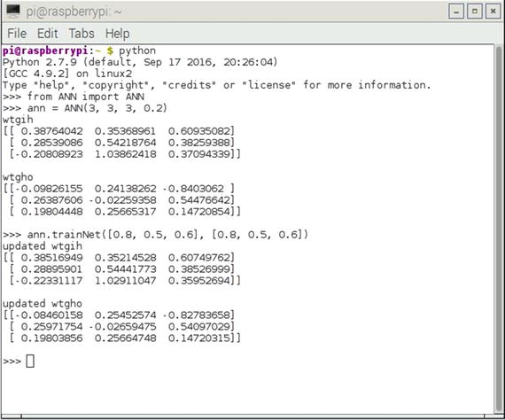
Figure 8-27. Interactive Python session

I have included several debug print statements in the ANN script, which allows for a direct comparison between the initial weight matrices and the updated ones. You should see there are only small changes between them, which is what was expected and desired. It is an important fact that the gradient descent works well using small increments to avoid missing the global minimum. I could only do one iteration in this session because the code was not set up for multiple iterations.

Congratulations for staying with me to this point! I covered a lot of topics concerning both ANN fundamentals and implementations. You should now be fully prepared to understand and appreciate the interesting practical ANN demonstrations presented in the next chapter.

Summary

This was the third of four chapters concerning artificial neural networks (ANNs). In this chapter, I focused on deep learning, which is really nothing more than the fundamentals and concepts behind multilayer ANNs.

After a brief review of some fundamentals, I completed a step-by-step manual calculation of a two-layer, six-node ANN. I subsequently redid the calculations using a Python script.

Next were the calculations for a larger, three-layer, nine-node ANN. Those calculations were done entirely with Python and matrix algorithms imported from the numpy library.

I discussed the errors that exist within an untrained ANN and how they are propagated. This was important to understand because it serves as the basis for the back propagation technique used to adjust weights in an effort to optimize the ANN.

Next, I went through a complete back propagation example, which illustrated how weights could be updated to reduce overall network errors. A sidebar followed wherein the gradient descent (GD) technique was introduced using a linear regression example.

A discussion involving the application of GD to an example ANN followed. The GD algorithm uses the slope of the error function in an effort to locate a global minimum, which is necessary to achieve a well-performing ANN.

I provided a complete example illustrating how to update weights using the GD algorithm. Issues with ANN learning and initial weight selection were discussed.

The chapter concluded with a thorough example of a Python script that initializes and trains any sized ANN.