This chapter starts an exploration into the broad topic of machine learning , which I introduced in Chapter 2. Machine learning is a hot topic in current industry and academia. Companies such as Google, Amazon, and Facebook have invested many millions of dollars in machine learning to improve their products and services. I begin with some fairly simple demonstrations on the Raspberry Pi to examine how a computer can “learn” in a primitive or naive sense. First, I would like to acknowledge that I drew much inspiration and knowledge for this chapter from Bert van Dam’s book Artificial Intelligence: 23 Projects to Bring Your Microcontroller to Life (Elektor Electronics Publishing, 2009). Although van Dam did not use a Raspberry Pi as a microcontroller, the concepts and techniques he applied are completely valid and especially appreciated.
Parts List
For the first demonstration, you need the parts listed in Table 6-1.
Table 6-1. Parts List
Description | Quantity | Remarks |
|---|---|---|
Pi Cobbler | 1 | 40-pin version, either T or DIP form factor acceptable |
solderless breadboard | 1 | 300 insertion points with power supply strips |
solderless breadboard | 1 | 300 insertion points |
jumper wires | 1 package | |
LED | 2 | green and yellow LEDs, if possible |
2.2kΩ resistor | 6 | 1/4 watt |
220Ω resistor | 2 | 1/4 watt |
10Ω resistor | 2 | 1/2 watt |
push button | 1 | tactile |
MCP3008 | 1 | 8-channel ADC chip DIP |
There is a robot demonstration discussed in this chapter that you can build by following the instructions in the appendix. It is also feasible to simply read the robot discussion and gain an appreciation of the concepts.
Demo 6-1: Color Selection
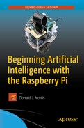
In this demonstration, you teach the computer your preferred color, which is either green or yellow. First, the Raspberry Pi must be set up according to the Fritzing diagram shown in Figure 6-1.
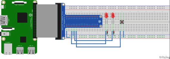
Figure 6-1. Fritzing diagram
Caution
Ensure that you connect one side of the push button switch to 3.3 V and not 5 V because you will destroy the GPIO pin if you inadvertently connect it to the higher voltage.
Next, I explain how the color selection algorithm works.
Algorithm
Consider the horizontal bar shown in Figure 6-2. It has a total numerical scale of 0 to 255. The left half of the bar has a scale of 0 to 127, which represents the green LED activation. The right half has a scale of 128 to 255, which represents the yellow LED activation.
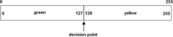
Figure 6-2. LED activation bar
Let’s create an integer random-number generator that produces a number between 0 and 255, inclusively. This is easily done with the following function, which I have used in previous Python programs:
decision = randint(0,255)randint() is the random integer generator method from the Python random library. The variable decision is a value between 0 and 255. If it is between 0 and 127, the green LED is lit; otherwise, the value is between 128 and 255, in which case the yellow LED is lit. Now, if the decision point remains unchanged, there is a 50/50 chance (or probability, over the long run) that the green LED lights up in each program repetition; there is an equal chance that the yellow LED will light. But that is not the goal of this program. The goal is to “teach” the program to select your favorite color. This goal can eventually be reached by moving the decision point so that it favors the favorite color selection. Let’s decide that green is the favorite color. Therefore, the decision point changes each time the green LED lights up because the user pressed the push button. This button press creates an interrupt with a callback function that increments the decision point value. Eventually, the decision point will be increased to such a value that just about every random number generated will fall within the green LED portion of the bar, as shown in Figure 6-3.
Figure 6-3. Adjusted number bar
The following program, named color_selection.py, implements the algorithm:
!/usr/bin/python# import statementsimport randomimport timeimport RPi.GPIO as GPIO# initialize global variable for decision pointglobal dpdp = 127# Setup GPIO pins# Set the BCM modeGPIO.setmode(GPIO.BCM)# OutputsGPIO.setup( 4, GPIO.OUT)GPIO.setup(17, GPIO.OUT)# InputGPIO.setup(27, GPIO.IN, pull_up_down = GPIO.PUD_DOWN)# Setup the callback functiondef changeDecisionPt(channel):global dpdp = dp + 1if dp == 255: # do not increase dp beyond 255dp =255# Add event detection and callback assignmentGPIO.add_event_detect(27, GPIO.RISING, callback=changeDecisionPt)while True:rn = random.randint(0,255)# useful to check on the dp valueprint 'dp = ', dpif rn <= dp:GPIO.output(4, GPIO.HIGH)time.sleep(2)GPIO.output(4, GPIO.LOW)else:GPIO.output(17, GPIO.HIGH)time.sleep(2)GPIO.output(17, GPIO.LOW)
Note
Press CTRL+C to exit the program.
When the program began, it was easy to see that the LEDs were on and off about equal amounts of time. However, as I continually pressed the push button, it rapidly became apparent that the green LED stayed lit for a longer time, until the dp value equaled 255 and the yellow LED never lit. The program thus “learned” that my favorite color was green.
But did the computer actually learn anything? This is more of a philosophical question than a technical one. It is the type of question that has continually bothered AI researchers and enthusiasts. I could easily restart the program, and the computer would reset the decision point and “forgot” the previous program execution. Likewise, I could change the program such that the dp value is stored externally in a separate data file that would load each time the program is run, thus remembering the favorite color selection. I will sidetrack the question of what computer learning actually means and focus on AI practicalities, as was the path taken by Dr. McCarthy, who I mentioned in Chapter 1.
The next section extends the concepts discussed in this simple demonstration.
Roulette Wheel Algorithm
Figure 6-4 shows a very simplified roulette wheel with four equal sectors (A through D), which represent events in a problem domain that compose the complete circle.
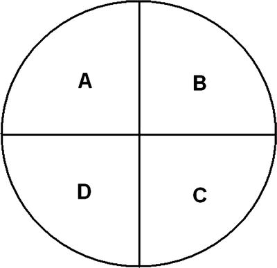
Figure 6-4. Simple roulette wheel
There is an average 0.25 probability that any segment will be selected on a given spin of the wheel. An equation to compute this event probability is directly related to the area of each segment. It can be expressed as follows:
A particular issue with using an equation such as this is that even though only p A may be needed, the representative areas B, C, and D must also be calculated to derive a valid probability for event A. From a computational point of view, it is very advantageous to focus on p A and not be concerned with the other event probabilities. All you really need to know is that a p A exists for the particular event A, and that it can be modified to accommodate a dynamic situation. In AI terminology, A, B, C, and D are known as fitness. In addition, the initial assumption is that all fitness ranges are equal, given that there is no apparent evidence to change this obvious choice.
It is somewhat easier to discuss fitness using a horizontal bar, as with the first example in this chapter. Figure 6-5 shows the fitness variables set in a horizontal bar, with 25 arbitrary values assigned to each one. Also shown on the bar are the results of three random draws, whose percentage values can range from 0 to 100. My selection of the individual fitness ranges makes it a one-to-one conversion with the draw percentages.
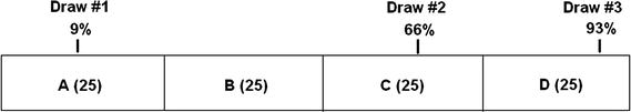
Figure 6-5. Four fitness variables with three random draws
The matching fitness for each draw is shown in Table 6-2.
Table 6-2. Initial Fitness Selection
Draw Number | Draw Percentage | Numerical Value | Fitness Selected |
|---|---|---|---|
1 | 9 | 9 | A |
2 | 60 | 60 | C |
3 | 93 | 93 | D |
However, let’s say that the initial assumption was wrong and that the four fitness ranges were not equal, but are as shown in Figure 6-6. The same draw percentages from Figure 6-5 are also shown.
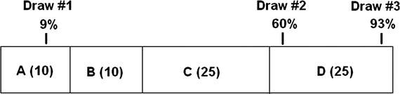
Figure 6-6. True fitness ranges
This new information changes the fitness choices, as displayed in Table 6-3.
Table 6-3. Modified Fitness Selection
Draw Number | Draw Percentage | Numerical Value | Fitness Selected |
|---|---|---|---|
1 | 9 | 6.3 | A |
2 | 60 | 42 | D |
3 | 93 | 65.1 | D |
The now reduced A and B fitness ranges leads to the draw #2 fitness choice, which changes from C to D. This scenario is precisely the same activity that happened in the color selection example, where every button press changed the decision point, which in-turn changed the fitness ranges for the two color selections.
Modifying the fitness range and the consequent selection of a strategy are the fundamental bases for the roulette wheel algorithm. As you will shortly learn, this algorithm is very useful in implementing a learning behavior for an autonomous vehicle, such as a small mobile robot. The roulette algorithm is used in medicine in the study of chromosome survival statistics, for example.
Demo 6-2: Autonomous Robot
Meet Alfie, a name I picked for my small mobile and autonomous robot. Alfie is pictured in Figure 6-7.
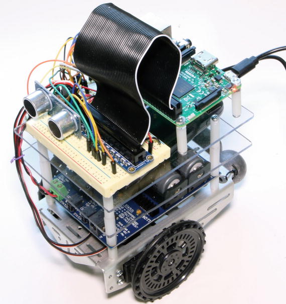
Figure 6-7. Alfie
I mentioned that the build instructions for Alfie are in the appendix. Feel free to read the following section without concern about all the tedious technical details involved in building the robot. However, you are certainly able to replicate this demonstration after you build and program Alfie.
The robot’s main task is to avoid all obstacles in its path. The path the robot takes is randomly generated in 2-second increments. Sometimes the path is straight ahead, whereas other times it is a circling motion to the left or right. Technically, the robot is not really avoiding obstacles because that would imply a predetermined path. It is avoiding all containment surfaces, actually, which are any nearby walls and doors.
The robot has an ultrasonic sensor that is beaming or “looking” forward. The objective is that if the ultrasonic sensor detects an obstacle, the robot must take immediate action to avoid it. The following are the only actions that the robot can take:
drive forward
turn left
turn right
There is no option for simply stopping. The robot must continue to move, even though it may not be the best option in a particular situation.
Autonomous Algorithm
Let’s start implementing the roulette wheel algorithm by arbitrarily assigning a fitness value of 20 to each of the actions. This initial value can be changed if it is found to be ineffective in the algorithm. Next, a random choice or draw is made. This draw is done every 2 seconds to prevent the robot from settling into a static behavior and not “learning” anything. I use the same 256 numerical range that was in the color selection example. The equation for a fitness selection is as follows:
![]()
randomInt ranges from 0 to 255.
The horizontal bar display for this setup is shown in Figure 6-8.
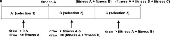
Figure 6-8. Robot roulette wheel fitness configuration
The fitness regions are continually updated and modified based on the robot’s activities and whether it has encountered an obstacle. Typically, if an obstacle is encountered, the fitness for the particular activity is decremented by one, thus slightly reducing its overall probability of being chosen in a draw. You can imagine that, over a long enough time span, all the activity finesses is reduced to 0. At that point, the robot is commanded to stop, essentially giving up in its quest to avoid obstacles.
The following code segment contains the initialization statements for all the component modules and the selection logic for the roulette wheel algorithm:
import RPi.GPIO as GPIOimport timeGPIO.setmode(GPIO.BCM)GPIO.setup(18, GPIO.OUT)GPIO.setup(19, GPIO.OUT)pwmL = GPIO.PWM(18,20) # pin 18 is left wheel pwmpwmR = GPIO.PWM(19,20) # pin 19 is right wheel pwm# must 'start' the motors with 0 rotation speedspwmL.start(2.8)pwmR.start(2.8)# ultrasonic sensor pinsTRIG = 23 # an outputECHO = 24 # an input# set the output pinGPIO.setup(TRIG, GPIO.OUT)# set the input pinGPIO.setup(ECHO, GPIO.IN)# initialize sensorGPIO.output(TRIG, GPIO.LOW)time.sleep(1)if fitA + fitB + fitC == 0:select = 0robotAction(select)elif draw >= 0 and draw <= fitA:select = 1robotAction(select)elif draw > fitA and draw <= (fitA + fitB):select = 2robotAction(select)elif draw > (fitA + fitB):select = 3robotAction(select)
The robotAction(select) method commands the robot to do one of the actions, or to stop in the extreme case where all the finesses have been reduced to 0. The selected robotAction is effective for only 2 seconds, until another draw is generated and an action is randomly selected. It could be the same as the one that just completed or one of the other two actions. The selection probabilities change as obstacles are encountered.
The following code implements the robotAction method :
def robotAction(select):if select == 0:# stop immediatelyexit()elif select == 1:pwmL.ChangeDutyCycle(3.6)pwmR.ChangeDutyCycle(2.2)elif select == 2:pwmL.ChangeDutyCycle(3.6)pwmR.ChangeDutyCycle(2.8)elif select == 3:pwmL.ChangeDutyCycle(2.8)pwmR.ChangeDutyCycle(2.2)
The robot program utilizes a polling routine to indicate when the robot is within 10 inches or 25.4 cm of an obstacle. This routine causes the robot to momentarily stop and then back up for 2 seconds, at which point a new draw is generated. In addition, the fitness that was in effect when the obstacle was detected is decremented by one unit. This activity is all set in an infinite loop, such that the robot continues to roam or reaches a quiescent state where it just rotates in place. All the fitness levels could also be reduced to 0, stopping it permanently.
The operation and wiring of the ultrasonic sensor is covered in the appendix, but now it is important to realize that when the ultrasonic sensor’s distance output values reach 10 inches or 25.4 cm, the polling routine will jump to the backup action and decrement the current active fitness sector.
The following code segment lists the distance calculation routine for the ultrasonic sensor:
# forever loop to continually generate distance measurementswhile True:# generate a 10 usec trigger pulseGPIO.output(TRIG, GPIO.HIGH)time.sleep(0.000010)GPIO.output(TRIG, GPIO.LOW)# following code detects the time duration for the echo pulsewhile GPIO.input(ECHO) == 0:pulse_start = time.time()while GPIO.input(ECHO) == 1:pulse_end = time.time()pulse_duration = pulse_end - pulse_start# distance calculationdistance = pulse_duration * 17150# round distance to two decimal pointsdistance = round(distance, 2)# for debugprint 'distance = ', dist, ' cm'# check for 25.4 cm distance or lessif distance < 25.40:backup()
The backup()method is only called if the detected distance falls below 10 inches or 25.4 cm. In this routine, the robot is commanded to move backward from whatever position it is in when the ultrasonic sensor polling routine triggers the method. The backup method also decrements the active fitness controlling the robot when the backup event is initiated. The following is the backup method listing:
def backup():global fitA, fitB, fitC, pwmL, pwmRif select == 1:fitA = fitA - 1if fitA < 0:fitA = 0elif select == 2:fitB = fitB - 1if fitB < 0:fitB = 0else:fitC = fitC -1if fitC < 0:fitC = 0# now, drive the robot in reverse for 2 secs.pwmL.ChangeDutyCycle(2.2)pwmR.ChangeDutyCycle(3.6)time.sleep(2) # unconditional time interval
I have now covered all the principal modules that make up the autonomous control program. The following listing combines all the modules into a comprehensive program. I also incorporated a time routine in the main loop that ensures that each of the robot actions selected by the draw is activated for 2 seconds. The ultrasonic sensor is also running while the robot actions are being performed. The only exception is when an obstacle is detected; this causes the robot to immediately stop what it is doing and back up for an unconditional 2 seconds. This program is named robotRoulette.py.
import RPi.GPIO as GPIOimport timefrom random import randintglobal pwmL, pwmR, fitA, fitB, fitC# initial fitness values for each of the 3 activitiesfitA = 20fitB = 20fitC = 20# use the BCM pin numbersGPIO.setmode(GPIO.BCM)# setup the motor control pinsGPIO.setup(18, GPIO.OUT)GPIO.setup(19, GPIO.OUT)pwmL = GPIO.PWM(18,20) # pin 18 is left wheel pwmpwmR = GPIO.PWM(19,20) # pin 19 is right wheel pwm# must 'start' the motors with 0 rotation speedspwmL.start(2.8)pwmR.start(2.8)# ultrasonic sensor pinsTRIG = 23 # an outputECHO = 24 # an input# set the output pinGPIO.setup(TRIG, GPIO.OUT)# set the input pinGPIO.setup(ECHO, GPIO.IN)# initialize sensorGPIO.output(TRIG, GPIO.LOW)time.sleep(1)# robotAction moduledef robotAction(select):global pwmL, pwmRif select == 0:# stop immediatelyexit()elif select == 1:pwmL.ChangeDutyCycle(3.6)pwmR.ChangeDutyCycle(2.2)elif select == 2:pwmL.ChangeDutyCycle(2.2)pwmR.ChangeDutyCycle(2.8)elif select == 3:pwmL.ChangeDutyCycle(2.8)pwmR.ChangeDutyCycle(2.2)# backup moduledef backup(select):global fitA, fitB, fitC, pwmL, pwmRif select == 1:fitA = fitA - 1if fitA < 0:fitA = 0elif select == 2:fitB = fitB - 1if fitB < 0:fitB = 0else:fitC = fitC -1if fitC < 0:fitC = 0# now, drive the robot in reverse for 2 secs.pwmL.ChangeDutyCycle(2.2)pwmR.ChangeDutyCycle(3.6)time.sleep(2) # unconditional time intervalclockFlag = False# forever loopwhile True:if clockFlag == False:start = time.time()randomInt = randint(0, 255)draw = (randomInt*(fitA + fitB + fitC))/255if fitA + fitB + fitC == 0:select = 0robotAction(select)elif draw >= 0 and draw <= fitA:select = 1robotAction(select)elif draw > fitA and draw <= (fitA + fitB):select = 2robotAction(select)elif draw > (fitA + fitB):select = 3robotAction(select)clockFlag = Truecurrent = time.time()# check to see if 2 seconds (2000ms) have elapsedif (current - start)*1000 > 2000:# this triggers a new draw at loop startclockFlag = False# generate a 10 μsec trigger pulseGPIO.output(TRIG, GPIO.HIGH)time.sleep(0.000010)GPIO.output(TRIG, GPIO.LOW)# following code detects the time duration for the echo pulsewhile GPIO.input(ECHO) == 0:pulse_start = time.time()while GPIO.input(ECHO) == 1:pulse_end = time.time()pulse_duration = pulse_end - pulse_start# distance calculationdistance = pulse_duration * 17150# round distance to two decimal pointsdistance = round(distance, 2)# check for 25.4 cm distance or lessif distance < 25.40:backup()
Test Run
I placed the robot in an L-shaped hallway in my home, where it was completely enclosed by walls and doors. The robot was powered by an external cell phone battery. I was able to SSH into the Raspberry Pi through my home Wi-Fi network. I started the program by entering the following command:
sudo python robotRoulette.pyThe robot immediately responded by making a turn, moving straight ahead, or backing up as it neared a wall or a door. It appeared that the robot essentially confined itself to an approximate 3 × 3 ft area, but there were occasional excursions. This behavior lasted for about 6 minutes when it began to move only in a back-and-forth motion, which probably meant the turning fitness sectors were reduced to 0, or near 0. After 7 minutes, the robot shut down as the program exited when all the fitness values finally equaled 0.
This test demonstrated that the robot did change its operational behavior based on dynamically changing fitness values. I will leave it up to you to call it learning or not.
What would you need to do if you wanted to add some additional learning to the robot car? That is the subject for the next section.
Additional Learning
It is critical to understand the basic requirements for learning if you want to add learning behaviors to the robot car. Just consider how the robot car changed its behavior in the previous example. First, the actions that the car is allowed to take were defined. They are pretty straightforward so there is really no learning involved at this point. Next, the fitness sectors were created and a randomized method of selecting a particular sector was implemented to actuate a consequent action. Again, no learning was involved. Finally, a sensor was incorporated into the scheme so that the sensor output could affect the fitness values, and ultimately, the robot’s behavior. That is where the learning kicks in. Thus learning, at least in this case, requires a sensor and a technique to modify the fitness values based on the sensor output. If you reflect on this for a moment, you recognize that this is the way humans also learn. It could be by reading a book where the eyes are the sensors, or listening to music where the ears are the primary sensors. It could even be the fingers of a small child touching a hot radiator.
It is therefore likely that we will either need a new sensor or somehow modify the existing one to implement additional learning. I elected to consider energy management to be the new learning behavior. Specifically, favoring those actions that minimize energy consumption to enhance the robot car’s learning potential.
Directly measuring energy consumption is difficult, but measuring energy used per unit of time is quite easy. Of course, energy used over a time period is simply power, which is easily computed using Ohm’s law:
![]()
or the equivalent:

A small resistor needs to be inserted into the motor power supply so that the current through it or the voltage drop across it can be measured. I elected to measure the voltage drop because it is compatible with the analog-to-digital converter chip that used with the Raspberry Pi to obtain sensor readings. The resistor value has to be quite small so as to not drop the motor supply voltage to the point that it would interfere with the required motor operation.
To determine the resistor value, I placed a VOM in series with the positive motor power supply lead and measured the average current while both motors were operating in the forward direction. The average current draw was about 190 ma. A series 5Ω resistor has about a 1 V drop with this current, while dissipating 0.2 W of power. The single volt drop should not have much of an impact on motor operation, considering that the maximum full-scale voltage output from the motor power supply is 7.5 V. The robot motors are nominally rated at 6 V, but can accept somewhat higher voltages without any harm. Higher voltages simply cause the motors to rotate faster.
The voltage drop across the resistor is measured using a MCP3008 multi-channel analog-to-digital converter (ADC). The setup and installation of this ADC chip is thoroughly covered in the robot build appendix. Two ADC channels are used because the differential voltage across the resistor is required to determine the current. Figure 6-9 is a schematic of the ADC connection with the current sense resistor.
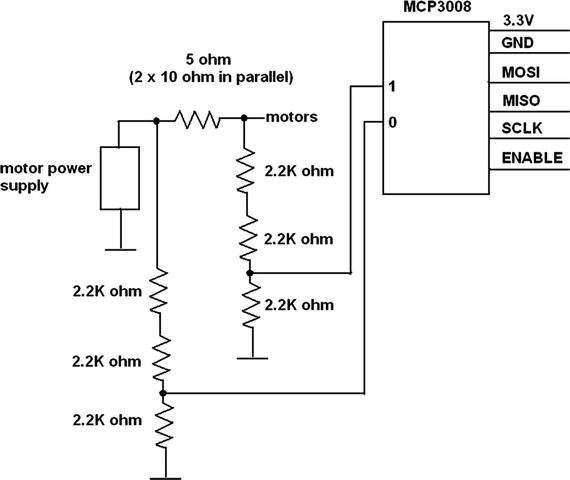
Figure 6-9. ADC connection to the current sense resistor
The following code is a test program that proves that the ADC is connected and functioning properly. It is a slight modification of the simpletest.py program sourced from the Adafruit Learn website:
# Import SPI library (for hardware SPI) and MCP3008 library.import Adafruit_GPIO.SPI as SPIimport Adafruit_MCP3008# Hardware SPI configuration:SPI_PORT = 0SPI_DEVICE = 0mcp = Adafruit_MCP3008.MCP3008(spi=SPI.SpiDev(SPI_PORT, SPI_DEVICE))print('Reading MCP3008 values, press Ctrl-C to quit...')# Print nice channel column headers.print('| {0:>4} | {1:>4} | {2:>4} | {3:>4} | {4:>4} | {5:>4} | {6:>4} | {7:>4} |'.format(*range(8)))print('-' * 57)# Main program loop.while True:# Read all the ADC channel values in a list.values = [0]*8for i in range(8):# The read_adc function will get the value of the specified channel (0-7).values[i] = mcp.read_adc(i)# Print the ADC values.print('| {0:>4} | {1:>4} | {2:>4} | {3:>4} | {4:>4} | {5:>4} | {6:>4} | {7:>4} |'.format(*values))# Pause for half a second.time.sleep(0.5)
Figure 6-10 is a screenshot of the program output after it ran for about 30 seconds.
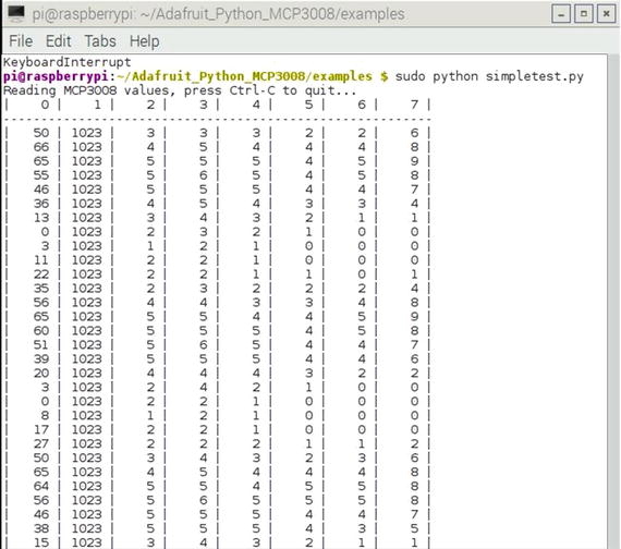
Figure 6-10. Test program output
Notice that channel 1 shows a consistent value of 1023 because it was tied to the 3.3 V supply. Vref is also tied to the 3.3 V supply, causing the maximum value to be 1023. This maximum value is a direct result of there being 10 bits in the conversion process. Also of interest is that channel 0 shows varying values, ranging from 0 to 66, while not connected to anything or basically floating. Channels 2 through 7 are also floating, but only display values from 0 to 9. It is my guess that there exists a high-impedance cross-coupling between channels 0 and 1, which is influencing the channel 0 reading. This coupling should not matter when channel 0 is actually connected to the sense resistor.
The actual total power computation requires the difference of two ADC readings from channels 0 and 1. Channel 0 is also the input motor supply voltage. I chose to use the absolute count difference across the resistor because there is almost an exact ratio of 1 count per millivolt thanks to the 1 V resistor drop and 1023 maximum ADC range. Both inputs use a voltage divider network that reduces the input voltage by two-thirds to keep them within the 3.3 V input range for the ADC chip. Theses voltage reductions are compensated for in the power calculation,
The total power dissipated includes the resistor power and the motor power. This value (expressed in watts) is computed as follows:
Let ![]()
This is also the resistor’s voltage drop.
The current is therefore![]()
Voltage drop across the motors:![]()

The next step is to consider how to integrate the power measurement and the energy consumption minimization approach into the existing robotRoulette program.
Demo 6-3: Adaptive Learning with an Energy Consumption Consideration
Minimizing energy consumption should be considered as a background activity for the robot car, instead of a primary activity such as driving forward or turning. The reason for this distinction is that all primary activities use energy, but some use less than others. Since all activities are involved with energy consumption, it makes no sense to create a separate fitness category for it. Instead, it is more logical to reward those activities that use less energy and to penalize activities that use more energy. The rewards and penalties take the form of slight adjustments to the respective activity fitness values. I arbitrarily decided that 0.5 points are added or subtracted to the fitness values depending upon whether the measured power level is above or below a preset milliwatt threshold value. This adjustment is included in the robotAction module. No other changes were made to the existing code except for inserting a new module that computes the power level. The new power module and modified robotAction modules are listed next.
global mcp, pwrThresholdpwrThreshold = 1000 # initial threshold value of 1000 mWdef calcPower:global mcpcount0 = mcp.read_adc(0)count1 = mcp.read_adc(1)diff = count0 - count1power = (3*count0*diff)/5return power# modified robotAction moduledef robotAction(select):global pwmL, pwmR, pwrThreshold, fitA, fitB, fitCif select == 0:# stop immediatelyexit()elif select == 1:pwmL.ChangeDutyCycle(3.6)pwmR.ChangeDutyCycle(2.2)if power() > pwrThreshold:fitA = fitA - 0.5else:fitA = fitA + 0.5elif select == 2:pwmL.ChangeDutyCycle(2.2)pwmR.ChangeDutyCycle(2.8)if power() > pwrThreshold:fitB = fitB - 0.5else:fitB = fitB + 0.5elif select == 3:pwmL.ChangeDutyCycle(2.8)pwmR.ChangeDutyCycle(2.2)if power() > pwrThreshold:fitC = fitC - 0.5else:fitC = fitC + 0.5
My expectation was that, on average, the energy consumption in the turning activities would be less than in driving forward. The reason is because only one motor is powered during a turn but two motors are powered while driving forward. This naturally leads to a gradual increase in both the fitB and fitC values, while the fitA value is reduced. Of course, the fitness adjustments related to obstacle detection are still taking place. My weighting of 0.5 fitness points for energy consumption makes that learning factor only 50 percent as effective as the obstacle-learning factor. I expected that the robot would eventually reach a quiescent state where it only turns in circles.
I renamed the main program to rre.py (short for robotRoulette_energy) after incorporating the modifications and the initializations needed to support the modifications . The complete listing follows.
import RPi.GPIO as GPIOimport timefrom random import randint# next two libraries must be installed IAW appendix instructionsimport Adafruit_GPIO.SPI as SPIimport Adafruit_MCP3008global pwmL, pwmR, fitA, fitB, fitC, pwrThreshold, mcp# Hardware SPI configuration:SPI_PORT = 0SPI_DEVICE = 0mcp = Adafruit_MCP3008.MCP3008(spi=SPI.SpiDev(SPI_PORT, SPI_DEVICE))# initial fitness values for each of the 3 activitiesfitA = 20fitB = 20fitC = 20#initial pwrThresholdpwrThreshold = 1000 # units of milliwatts# use the BCM pin numbersGPIO.setmode(GPIO.BCM)# setup the motor control pinsGPIO.setup(18, GPIO.OUT)GPIO.setup(19, GPIO.OUT)pwmL = GPIO.PWM(18,20) # pin 18 is left wheel pwmpwmR = GPIO.PWM(19,20) # pin 19 is right wheel pwm# must 'start' the motors with 0 rotation speedspwmL.start(2.8)pwmR.start(2.8)# ultrasonic sensor pinsTRIG = 23 # an outputECHO = 24 # an input# set the output pinGPIO.setup(TRIG, GPIO.OUT)# set the input pinGPIO.setup(ECHO, GPIO.IN)# initialize sensorGPIO.output(TRIG, GPIO.LOW)time.sleep(1)# modified robotAction moduledef robotAction(select):global pwmL, pwmR, pwrThreshold, fitA, fitB, fitCif select == 0:# stop immediatelyexit()elif select == 1:pwmL.ChangeDutyCycle(3.6)pwmR.ChangeDutyCycle(2.2)if calcPower() > pwrThreshold:fitA = fitA - 0.5else:fitA = fitA + 0.5elif select == 2:pwmL.ChangeDutyCycle(2.2)pwmR.ChangeDutyCycle(2.8)if calcPower() > pwrThreshold:fitB = fitB - 0.5else:fitB = fitB + 0.5elif select == 3:pwmL.ChangeDutyCycle(2.8)pwmR.ChangeDutyCycle(2.2)if calcPower() > pwrThreshold:fitC = fitC - 0.5else:fitC = fitC + 0.5# backup moduledef backup(select):global fitA, fitB, fitC, pwmL, pwmRif select == 1:fitA = fitA - 1if fitA < 0:fitA = 0elif select == 2:fitB = fitB - 1if fitB < 0:fitB = 0else:fitC = fitC -1if fitC < 0:fitC = 0# now, drive the robot in reverse for 2 secs.pwmL.ChangeDutyCycle(2.2)pwmR.ChangeDutyCycle(3.6)time.sleep(2) # unconditional time interval# power calculation moduledef calcPower:global mcpcount0 = mcp.read_adc(0)count1 = mcp.read_adc(1)count2 = mcp.read_adc(2)diff = count0 - count1power = (3*count0*diff)/5return powerclockFlag = False# forever loopwhile True:if clockFlag == False:start = time.time()randomInt = randint(0, 255)draw = (randomInt*(fitA + fitB + fitC))/255if fitA + fitB + fitC == 0:select = 0robotAction(select)elif draw >= 0 and draw <= fitA:select = 1robotAction(select)elif draw > fitA and draw <= (fitA + fitB):select = 2robotAction(select)elif draw > (fitA + fitB):select = 3robotAction(select)clockFlag = Truecurrent = time.time()# check to see if 2 seconds (2000ms) have elapsedif (current - start)*1000 > 2000:# this triggers a new draw at loop startclockFlag = False# generate a 10 μsec trigger pulseGPIO.output(TRIG, GPIO.HIGH)time.sleep(0.000010)GPIO.output(TRIG, GPIO.LOW)# following code detects the time duration for the echo pulsewhile GPIO.input(ECHO) == 0:pulse_start = time.time()while GPIO.input(ECHO) == 1:pulse_end = time.time()pulse_duration = pulse_end - pulse_start# distance calculationdistance = pulse_duration * 17150# round distance to two decimal pointsdistance = round(distance, 2)# check for 25.4 cm distance or lessif distance < 25.40:backup()
Test Run
I placed the robot in the same hallway as the previous test run. I initiated another SSH session and started the program by the entering the following command:
sudo python rre.py The robot immediately responded, as it did previously, by making a turn, moving straight ahead, or backing up as it neared a wall or door. The motions were fairly well mixed. After approximately 5 minutes, the vast majority of motions were the turning actions, with only an occasional straight-ahead action. The backups only happened if the robot came too close to a wall while turning. It certainly became apparent to me that the robot had “learned” that turning motions were indeed the best way to conserve energy.
This project concludes this chapter’s focus on machine learning. The next chapter takes machine leaning to a much deeper level.
Summary
This chapter is the first of several that explore the highly interesting topic of machine learning. The first Raspberry Pi demonstration involved the user pressing a push button whenever the favored LED randomly lit. Before long, the computer “learned” the favorite color and consistently lit that particular LED. The concept of fitness was introduced in this project.
I next discussed the roulette wheel algorithm, which was a prelude to the next demonstration of an autonomous robot car that incorporated learning behaviors. Alfie, the robot car, performed a few selected actions or behaviors, which eventually became either reinforced or diminished, depending on whether the car encountered an obstacle while performing the action. Eventually, the car reached a quiescent state where it could not perform any actions and it simply shut down.
The final demonstration illustrated how to add another behavior to the robot car. This new behavior focused on energy conservation. The car rapidly learned to favor those actions that consumed less energy than the ones that consumed more than the preset threshold.