Python Script

Credit must go to Will Larson. I am using his code from a 2009 article entitled “Genetic Algorithms: Cool Name & Damn Simple” ( https://lethain.com/genetic-algorithms-cool-name-damn-simple/ ) from his blog, which is called Irrational Exuberance. I highly recommend that you take a look at it.

The problem to be solved is the same one used in the manual calculations section on determining six integers with values ranging from 0 to 100 and summing to a target value of 371.

The first item to consider in formulating a solution is how to structure it to fit into the EC paradigm. There are individuals to create who will eventually form a population. The individuals for this specific case will be six element lists consisting of integers whose values range from 0 to 100. Multiple individuals make up a population. The following code segment creates the individuals:

from random import randint
def individual(length, min, max):
    # generates an individual
    return [randint(min, max) for x in xrange(length)]

Figure 10-1 shows an interactive Python session where I generated several individuals.

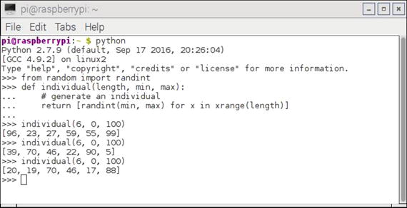
Figure 10-1. Interactive Python session individual generation

The individuals generated must be collected so that they form a population, which is the next part of the solution structure. The following code segment generates a population. This segment depends upon the previous code segment to have already been entered:

def population(count, length, min, max):
    # generate a population
    return [individual(length, min, max) for x in xrange(count)]

Figure 10-2 shows an interactive Python session where I generated several populations.

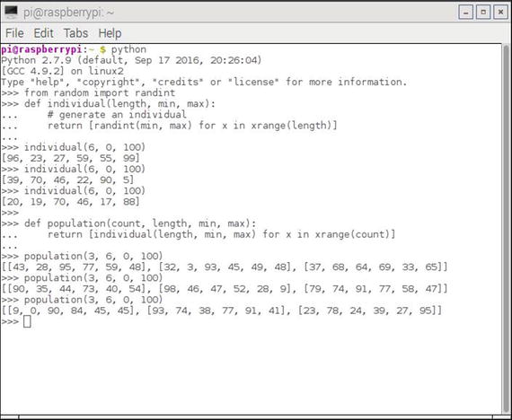
Figure 10-2. Interactive Python session population generation

The next step in this process is to create a function that measures how well a particular individual performs in meeting the stated objective (i.e., integer lists values summing to a target value). This function is called a fitness function. Note that the fitness function requires the individual function to have been previously entered. The following is a code segment implementation for the fitness function:

from operator import add
def fitness(individual, target):
    # calculate fitness, lower the better
    sum = reduce(add, individual, 0)
    return abs(target - sum)

Figure 10-3 shows an interactive Python session where I tested several individuals against a constant target value.

Figure 10-3. Interactive Python session fitness tests

This particular fitness function is much simpler than similar fitness tests that I have demonstrated in past chapters. In this one, only the absolute value of the difference between the summed elements contained in an individual list and a target value is calculated. The best case would be a 0.0 value, which I will shortly demonstrate.

The only missing element in the structure is how to change or evolve the population to meet the objective. Only by the purest luck would an initial solution also be an optimal solution. There must be a strategy stated to properly implement an evolutionary function. The following is the strategy set forth for this structure :

• Take 20% of the top performers (elitism rate) from a prior population and include them in a new one.

• Breed approximately 75% of the new population as children.

• Take the first length/2 elements from a father and the last length/2 elements from a mother to form a child.

• It is forbidden to have a father and a mother as the same individual.

• Randomly select 5% from the population.

• Mutate 1% of the new population.

This strategy is by no means a standard one, or even a very comprehensive one, but it will suffice for this problem and it is fairly representative of those used for similar problems.

Figure 10-4 is an interactive Python session that shows how children are formed in this strategy.

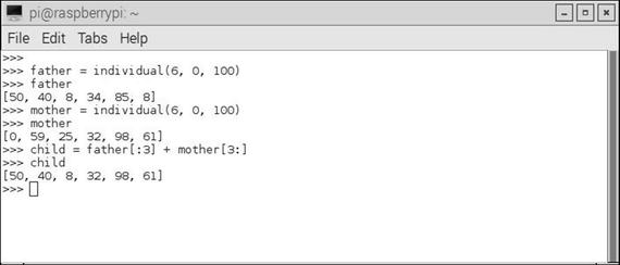
Figure 10-4. Forming children for a new population

The mutating part of the strategy is a bit more complex, which I show, in part, with the next code segment before trying to explain it:

from random import random, randint
chance_to_mutate = 0.01
for i in population:
    if chance_to_mutate > random():
        place_to_mutate = randint(0, len(i))
        i[place_to_mutate] = randint(min(i), max(i))
...
...

The chance_to_mutate variable is set to 0.01, representing a 1% chance for mutation, which is very low as I noted earlier. The statement for i in population: iterates through the entire population and causes a mutation only when the random number generator is less than .01, which is not very often. The actual individual chosen to be mutated is accomplished by the place_to_mutate = randint(0, len(i)) statement, which is not likely the individual that happened to be iterated upon at the time the random number was less than .01. Finally, the actual mutation is done by this statement: i[place_to_mutate] = randint(min(i), max(i)). The integer values in the selected individual are randomly generated based upon the population’s min and max values.

The whole strategy design, which includes a mix of selecting the best-performing individuals, breeding children from all portions of the population, and the occasional mutations is geared toward finding the global maximum and avoiding local maximums. This is precisely the same thought process that was going on in the gradient descent algorithm for ANNs, where the goal was to locate a global minimum and avoid local minimums. You can look at Figure 8-15 to visualize the process for locating the global maximum or highest peak instead of the deepest valley, representing the global minimum.

There is much more to the evolve function than what was shown. The remaining code is shown next in the complete script listing.

There is one more function to explain before the complete script is shown. This function is named grade and it calculates an overall fitness measure for a whole population. The Python built-in reduce function sums the fitness scores for each individual and averages the sum by the population size. The following code implements the grade function :

def grade(pop, target):
    'Find average fitness for a population.'
    summed = reduce(add, (fitness(x, target) for x in pop))
    return summed / (len(pop) * 1.0)

This last function listing concludes my discussion on all the functions that compose the Python script. The following is a complete listing of the final script, along with instructions on how to run the script within an interactive Python session. Note that I did modify the instructions to display the first generation number that met the target and the final solution itself. The population in the example is equal to 100 and each individual has six elements with values ranging between 0 and 100.

"""
# Example usage
>>> from genetic import *
>>> target = 371
>>> p_count = 100
>>> i_length = 6
>>> i_min = 0
>>> i_max = 100
>>> p = population(p_count, i_length, i_min, i_max)
>>> fitness_history = [grade(p, target),]
>>> fitFlag = 0
>>> for i in xrange(100):
...    p = evolve(p, target)
...    fitness_history.append(grade(p, target))
...    if grade(p, target) == 0:
...        if fitFlag == 0:
...            fitFlag = 1
...            print 'Generation = ', i
...            print p[0]
>>> for datum in fitness_history:
...    print datum
"""

from random import randint, random
from operator import add

def individual(length, min, max):
    'Create a member of the population.'
    return [ randint(min,max) for x in xrange(length) ]

def population(count, length, min, max):
    """
    Create a number of individuals (i.e. a population).

    count: the number of individuals in the population
    length: the number of values per individual
    min: the minimum possible value in an individual's list of values
    max: the maximum possible value in an individual's list of values

    """
    return [ individual(length, min, max) for x in xrange(count) ]

def fitness(individual, target):
    """
    Determine the fitness of an individual. Higher is better.

    individual: the individual to evaluate
    target: the target number individuals are aiming for
    """
    sum = reduce(add, individual, 0)
    return abs(target-sum)

def grade(pop, target):
    'Find average fitness for a population.'
    summed = reduce(add, (fitness(x, target) for x in pop))
    return summed / (len(pop) * 1.0)

def evolve(pop, target, retain=0.2, random_select=0.05, mutate=0.01):
    graded = [ (fitness(x, target), x) for x in pop]
    graded = [ x[1] for x in sorted(graded)]
    retain_length = int(len(graded)*retain)
    parents = graded[:retain_length]
    # randomly add other individuals to
    # promote genetic diversity
    for individual in graded[retain_length:]:
        if random_select > random():
            parents.append(individual)
    # mutate some individuals
    for individual in parents:
        if mutate > random():
            pos_to_mutate = randint(0, len(individual)-1)
            # this mutation is not ideal, because it
            # restricts the range of possible values,
            # but the function is unaware of the min/max
            # values used to create the individuals,
            individual[pos_to_mutate] = randint(
                min(individual), max(individual))
    # crossover parents to create children
    parents_length = len(parents)
    desired_length = len(pop) - parents_length
    children = []
    while len(children) < desired_length:
        male = randint(0, parents_length-1)
        female = randint(0, parents_length-1)
        if male != female:
            male = parents[male]
            female = parents[female]
            half = len(male) / 2
            child = male[:half] + female[half:]
            children.append(child)
    parents.extend(children)
    return parents

Figure 10-5 shows an interactive session in which I entered all the statements shown in the instructions portion of the script comments.

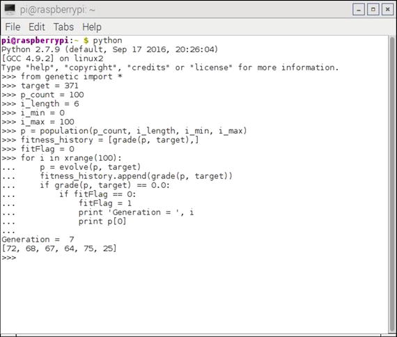
Figure 10-5. Interactive Python session running the script

You should be able to see in the screenshot that a solution was found after only seven generations had evolved. The solution was [72, 68, 67, 64, 75, 25], which does sum to the target value of 371. The script does not stop after the first successful solution is found, but continues to evolve and mutate, slightly degrading and then improving until it has run through its preset cycle number.

A portion of the history of the fitness numbers associated with each generation is shown in Figure 10-6.

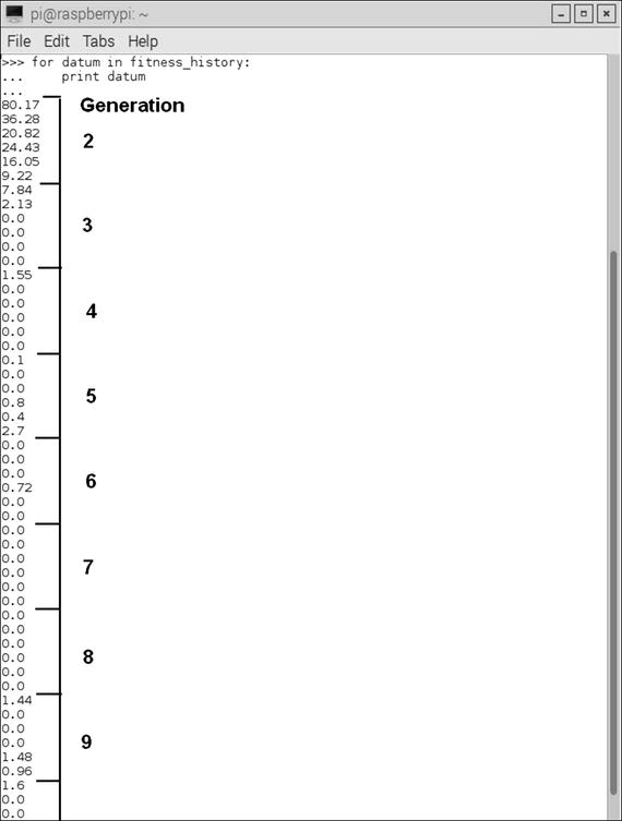
Figure 10-6. Fitness history list

In Figure 10-6, I annotated where generation 7 has a 0.0 fitness value for each of its individuals. Overall, this genetic programming approach is very efficient, especially for the relatively simple objective of determining a target sum given a list of six randomly generated integer numbers.

The next demonstration is a slight variant from Conway’s Game of Life, which is a classic project incorporating genetic programming with artificial life (alife) that breed and die according to a set of conditions based on their proximity to each other, which I explain later.

Sense HAT Hardware Installation

First, ensure that the Raspberry Pi is completely powered down. The Sense HAT is designed to mount on top of a Raspberry Pi. It comes with a 40-pin GPIO male pin extension header that you must first plug into the female 40-pin header on the Raspberry Pi. The Sense HAT is then mounted on top of the Raspberry Pi using the 40 male pins as a guide. These pins should simply push through the 40-pin female header on the Sense board. All that’s left is to attach the supplied stand-offs, which provide firm support between the Raspberry Pi and the Sense HAT. Figure 10-8 shows a mounted Sense HAT on a Raspberry Pi.

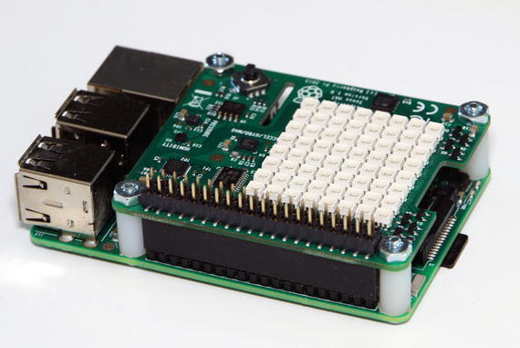
Figure 10-8. Sense HAT mounted onto a Raspberry Pi

There is one more item that you should know. The Raspberry Pi and Sense HAT require a power supply capable of providing 2.5A at 5V. Failing to use a sufficiently powerful power supply will likely cause strange behavior, such as the Linux OS failing to recognize the Sense HAT, which I unfortunately confirmed as a fact.

Sense HAT Software Installation

The Python library supporting the Sense HAT must be loaded prior to running any of the scripts that will run the Life game. First, ensure that the Raspberry Pi is connected to the Internet, and then enter the following commands to load the software:

sudo apt-get update
sudo apt-get install sense-hat
sudo reboot

You want to run the following test to ensure that the Sense HAT is working properly with the newly installed software. Enter the following in an interactive Python session:

from sense_hat import SenseHat
sense = SenseHat()
sense.show_message("Hello World!")

If all went well with the installation, you show see the Hello World! message scrolling across the LED array. If you don’t see it, I would recheck that the Sense HAT is securely fastened to the Raspberry Pi and that all 40 pins go through their respective socket holes. It very well might be that you inadvertently bent one of the pins such that it is has been forced out of the way. If that’s the case, just carefully straighten it and reseat all the pins.

Once the software checks out, you are ready to run a Python version of the Game of Life on this combination of Sense HAT/Raspberry Pi. I now turn the discussion to the game software.

Game of Life: Python Version

I begin this section by giving credit to Mr. Swee Meng Ng, a very talented Malaysian developer who posted much of the code I used in this project on GitHub.com. Swee goes by the username sweemeng on GitHub. He has a blog at www.nomadiccodemonkey.com . Take a look at it if you want an appreciation for the code development efforts that are ongoing in that part of the world.

You should first load the following Python scripts from https://github.com/sweemeng/sweemengs-game-of-life.git into your home directory:

• genelab.ppy

• designer.py

• gameoflife.py

genelab.py is the first script that I’ll discuss. It is the main one in this application. By main, I mean it incorporates the starting point, initialization, generation creation, and mutation, and finally, it enforces the behavioral rules. However, this script needs two helper scripts to work properly. These helper scripts are named designer.py and gameoflife.py, which I discuss shortly. I have added my own comments to Swee Meng’s scripts to help relate portions of it to concepts that have already been discussed, and hopefully, to clarify the purpose of the code segments.

import random
import time
# first helper
from designer import CellDesigner
from designer import GeneBank
# second helper
from gameoflife import GameOfLife
# not exactly a helper but needed for the display
from sense_hat import SenseHat

# you can customize your colors here
WHITE = [ 0, 0, 0 ]
RED = [ 120, 0, 0 ]

# begin class definition
class Genelab(object):
    # begin initialization
    def __init__(self):
        self.survive_min = 5 # Cycle
        self.surival_record = 0
        self.designer = CellDesigner()
        self.gene_bank = GeneBank()
        self.game = GameOfLife()
        self.sense = SenseHat()

    # random starting point
    def get_start_point(self):
        x = random.randint(0, 7)
        y = random.randint(0, 7)
        return x, y

    # create a fresh generation (population)
    # or mutate an existing one
    def get_new_gen(self):
        if len(self.gene_bank.bank) == 0:
            print("creating new generation")
            self.designer.generate_genome()
        elif len(self.gene_bank.bank) == 1:
            print("Mutating first gen")
            self.designer.destroy()
            seq_x = self.gene_bank.bank[0]
            self.designer.mutate(seq_x)
        else:
            self.designer.destroy()
            coin_toss = random.choice([0, 1])
            if coin_toss:
                print("Breeding")
                seq_x = self.gene_bank.random_choice()
                seq_y = self.gene_bank.random_choice()
                self.designer.cross_breed(seq_x, seq_y)
            else:
                print("Mutating")
                seq_x = self.gene_bank.random_choice()
                self.designer.mutate(seq_x)

    # a method to start the whole game, i.e. lab.run()
    def run(self):
        self.get_new_gen()
        x, y = self.get_start_point()
        cells = self.designer.generate_cells(x, y)
        self.game.set_cells(cells)
        # count is the generation number
        count = 1
        self.game.destroy_world()
        # forever loop. Change this if you only want a finite run
        while True:
            try:
                # essentially where the rules are applied
                if not self.game.everyone_alive():
                    if count > self.survive_min:
                        # Surivival the fittest
                       self.gene_bank.add_gene(self.designer.genome)
                        self.survival_record = count

                    print("Everyone died, making new gen")
                    print("Species survived %s cycle" % count)
                    self.sense.clear()
                    self.get_new_gen()
                    x, y = self.get_start_point()
                    cells = self.designer.generate_cells(x, y)
                    self.game.set_cells(cells)
                    count = 1

                if count % random.randint(10, 100) == 0:
                    print("let's spice thing up a little")
                    print("destroying world")
                    print("Species survived %s cycle" % count)
                    self.game.destroy_world()
                    self.gene_bank.add_gene(self.designer.genome)
                    self.sense.clear()
                    self.get_new_gen()
                    x, y = self.get_start_point()
                    cells = self.designer.generate_cells(x, y)
                    self.game.set_cells(cells)
                    count = 1

                canvas = []

                 # this where the cells are "painted" onto the canvas
                 # The canvas is based on the grid pattern from the
                # gameoflife script
                for i in self.game.world:
                    if not i:
                        canvas.append(WHITE)
                    else:
                        canvas.append(RED)
                self.sense.set_pixels(canvas)
                self.game.run()
                count = count + 1
                time.sleep(0.1)
            except:
                print("Destroy world")
                print("%s generation tested" % len(self.gene_bank.bank))
                self.sense.clear()
                break

if __name__ == "__main__":
    # instantiate the class GeneLab
    lab = Genelab()
    # start the game
    lab.run()

The first helper script is designer.py. The code listing follows with the addition of my own comments:

import random

class CellDesigner(object):
    # initialization
    def __init__(self, max_point=7, max_gene_length=10, genome=[]):
        self.genome = genome
        self.max_point = max_point
        self.max_gene_length = max_gene_length

    # a genome is made up of 1 to 10 genes
    def generate_genome(self):
        length = random.randint(1, self.max_gene_length)
        print(length)
        for l in range(length):
            gene = self.generate_gene()
            self.genome.append(gene)

    # a gene is an (+/-x, +/-y) cooordinate pair; x, y range 0 to 7
    def generate_gene(self):
        x = random.randint(0, self.max_point)
        y = random.randint(0, self.max_point)
        x_dir = random.choice([1, -1])
        y_dir = random.choice([1, -1])
        return ((x * x_dir), (y * y_dir))

    def generate_cells(self, x, y):
        cells = []
        for item in self.genome:
            x_move, y_move = item

            new_x = x + x_move
            if new_x > self.max_point:
                new_x = new_x - self.max_point
            if new_x < 0:
                new_x = self.max_point + new_x

            new_y = y + x_move
            if new_y > self.max_point:
                new_y = new_y - self.max_point
            if new_y < 0:
                new_y = self.max_point + new_y
            cells.append((new_x, new_y))
        return cells

    def cross_breed(self, seq_x, seq_y):
        if len(seq_x) > len(seq_y):
            main_seq = seq_x
            secondary_seq = seq_y
        else:
            main_seq = seq_y
            secondary_seq = seq_x

        for i in range(len(main_seq)):
            gene = random.choice([ main_seq, secondary_seq ])
            if i > len(gene):
                continue
            self.genome.append(gene[i])

    def mutate(self, sequence):
        # Just mutate one gene
        for i in sequence:
            mutate = random.choice([ True, False ])
            if mutate:
                gene = self.generate_gene()
                self.genome.append(gene)
            else:
                self.genome.append(i)

    def destroy(self):
        self.genome = []

class GeneBank(object):
    def __init__(self):
        self.bank = []

    def add_gene(self, sequence):
        self.bank.append(sequence)

    def random_choice(self):
        if not self.bank:
            return None
        return random.choice(self.bank)

The second helper script is gameoflife.py. There is only a small portion of this script that is actually used as a helper for the main script. I have included it all for the sake of completeness and to provide you with the code, in case you want to run a single-generation Game of Life, which I will explain shortly. The complete code listing follows with my own comments added:

import time
world = [
    0, 0, 0, 0, 0, 0, 0, 0,
    0, 0, 0, 0, 0, 0, 0, 0,
    0, 0, 0, 0, 0, 0, 0, 0,
    0, 0, 0, 0, 0, 0, 0, 0,
    0, 0, 0, 0, 0, 0, 0, 0,
    0, 0, 0, 0, 0, 0, 0, 0,
    0, 0, 0, 0, 0, 0, 0, 0,
    0, 0, 0, 0, 0, 0, 0, 0,
]

max_point = 7 # We use a square world to make things easy

class GameOfLife(object):
    def __init__(self, world=world, max_point=max_point, value=1):
        self.world = world
        self.max_point = max_point
        self.value = value

    def to_reproduce(self, x, y):
        if not self.is_alive(x, y):
            neighbor_alive = self.neighbor_alive_count(x, y)
            if neighbor_alive == 3:
                return True
        return False

    def to_kill(self, x, y):
        if self.is_alive(x, y):
            neighbor_alive = self.neighbor_alive_count(x, y)
            if neighbor_alive < 2 or neighbor_alive > 3:
                return True
        return False

    def to_keep(self, x, y):
        if self.is_alive(x, y):
            neighbor_alive = self.neighbor_alive_count(x, y)
            if neighbor_alive >= 2 and neighbor_alive <= 3:
                return True
        return False

    def is_alive(self, x, y):
        pos = self.get_pos(x, y)
        return self.world[pos]

    def neighbor_alive_count(self, x, y):

        neighbors = self.get_neighbor(x, y)
        alives = 0
        for i, j in neighbors:
            if self.is_alive(i, j):
                alives = alives + 1
        # Because neighbor comes with self, just for easiness
        if self.is_alive(x, y):
            return alives - 1
        return alives

    def get_neighbor(self, x, y):
        #neighbors = [
        #    (x + 1, y + 1), (x, y + 1), (x - 1, y + 1),
        #    (x + 1, y),     (x, y),     (x, y + 1),
        #    (x + 1, y - 1), (x, y - 1), (x - 1, y - 1),
        #]
        neighbors = [
            (x - 1, y - 1), (x - 1, y), (x - 1, y + 1),
            (x, y - 1),     (x, y),     (x, y + 1),
            (x + 1, y - 1), (x + 1, y), (x + 1, y + 1)
        ]
        return neighbors

    def get_pos(self, x, y):
        if x < 0:
            x = max_point
        if x > max_point:
            x = 0
        if y < 0:
            y = max_point
        if y > max_point:
            y = 0

        return (x * (max_point+1)) + y

    # I am seriously thinking of having multiple species
    def set_pos(self, x, y):
        pos = self.get_pos(x, y)
        self.world[pos] = self.value

    def set_cells(self, cells):
        for x, y in cells:
            self.set_pos(x, y)

    def unset_pos(self, x, y):
        pos = self.get_pos(x, y)
        self.world[pos] = 0

    def run(self):
        something_happen = False
        operations = []
        for i in range(max_point + 1):
            for j in range(max_point + 1):
                if self.to_keep(i, j):
                    something_happen = True
                    continue
                if self.to_kill(i, j):
                    operations.append((self.unset_pos, i, j))
                    something_happen = True
                    continue
                if self.to_reproduce(i, j):
                    something_happen = True
                    operations.append((self.set_pos, i, j))
                    continue
        for func, i, j in operations:
            func(i, j)
        if not something_happen:
            print("weird nothing happen")

    def print_world(self):
         count = 1
         for i in self.world:

            if count % 8 == 0:
                print("%s " %i)
            else:
                print("%s " %i) #, end = "")
            count = count + 1
         print(count)

    def print_neighbor(self, x, y):
        neighbors = self.get_neighbor(x, y)
        count = 1
        for i, j in neighbors:
            pos = self.get_pos(i, j)
            if count %3 == 0:
                print("%s " %self.world[pos])
            else:
                print("%s " %self.world[pos]) #, end = "")
            count = count + 1
        print(count)

    def everyone_alive(self):
        count = 0
        for i in self.world:
            if i:
                count = count + 1
        if count:
            return True
        return False

    def destroy_world(self):
        for i in range(len(self.world)):
            self.world[i] = 0

def main():
    game = GameOfLife()
    cells = [ (2, 4), (3, 5), (4, 3), (4, 4), (4, 5) ]
    game.set_cells(cells)
    print(cells)
    while True:
        try:
            game.print_world()

            game.run()
            count = 0
            time.sleep(5)
        except KeyboardInterrupt:
            print("Destroy world")
            break

def debug():
    game = GameOfLife()
    cells = [ (2, 4), (3, 5), (4, 3), (4, 4), (4, 5) ]
    game.set_cells(cells)
    test_cell = (3, 3)
    game.print_neighbor(*test_cell)
    print("Cell is alive: %s" % game.is_alive(*test_cell))
    print("Neighbor alive: %s" % game.neighbor_alive_count(*test_cell))
    print("Keep cell: %s" % game.to_keep(*test_cell))
    print("Make cell: %s" % game.to_reproduce(*test_cell))
    print("Kill cell: %s" % game.to_kill(*test_cell))
    game.print_world()
    game.run()
    game.print_world()

if __name__ == "__main__":
    main()
    #debug()

Test Run

First, ensure that the genelab.py , designer.py, and gameoflife.py scripts are in the pi home directory before running this command:

python genelab.py

The Raspberry takes a moment to load everything. You should begin to see the cells appear on the Sense HAT LED array, as well as status messages on the console screen. Figure 10-9 is a photograph of the LED array while my script was running.

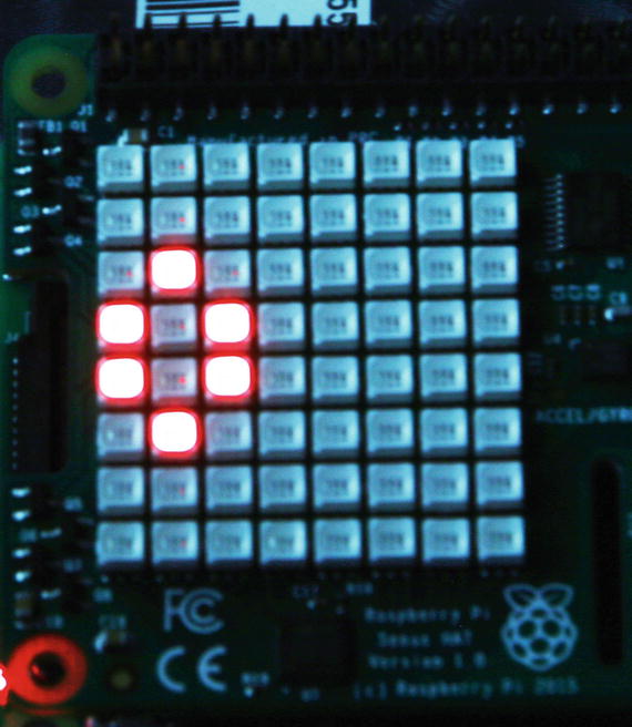
Figure 10-9. Sense HAT LED array with the Game of Life running

Figure 10-10 shows the console display while the game was running.

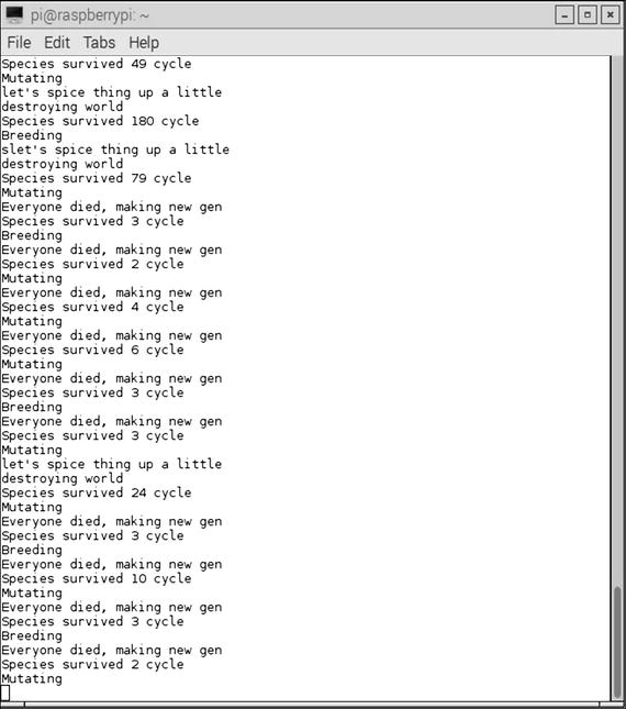
Figure 10-10. Console display with the Game of Life running

Single Generation of the Game of Life

It is also entirely possible to experiment with only a single generation of the Game of Life. This script simply adheres to the rules for the cell neighbors that were previously specified, with no cell or gene mutations allowed. The following script is named main.py. It is available on the same GitHub website as the previous scripts.

from sense_hat import SenseHat
from gameoflife import GameOfLife
import time
                                                                                                        
WHITE = [ 0, 0, 0 ]
RED = [ 255, 0, 0 ]

def main():

    game = GameOfLife()

    sense = SenseHat()
    # cells = [(2, 4), (3, 5), (4, 3), (4, 4), (4, 5)]
    cells = [(2, 4), (2, 5), (1,5 ), (1, 6), (3, 5)]
    game.set_cells(cells)

    while True:
        try:
            canvas = []
            for i in game.world:
                if not i:
                    canvas.append(WHITE)
                else:
                    canvas.append(RED)
            sense.set_pixels(canvas)
            game.run()
            if not game.everyone_alive():
                sense.clear()
                print("everyone died")
                break
            time.sleep(0.1)
        except:
            sense.clear()
            break

if __name__ == "__main__":
    main()

Enter the following command to run this script:

python main.py

The initial cell configuration is set by this statement:

cells = [(2, 4), (2, 5), (1, 5), (1, 6), (3, 5)]

You can try another configuration by uncommenting the prior cells array, and then comment out this one. I did that very action and then ran the script. I observed an unusual display, which I will not describe. I will leave it for you to discover.

I want to caution that what I am about to describe can become quite addictive. It is testing the consequences of new initial starting patterns. There are more than a few AI researchers who have dedicated their careers to the study of cellular automata, which includes researching the fascinating evolving patterns from the Game of Life.

Figure 10-11 illustrates some starting configurations that you may wish to try. The companion cell configuration array values are shown next to each of the patterns.

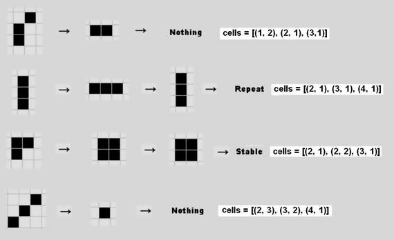
Figure 10-11. Example Game of Life starting patterns

Two of the patterns immediately disappear (die), one goes into a bi-stable state, and the fourth pattern enters a stable state. I tested each pattern and confirmed it acted as shown.

Figure 10-12 shows other initial patterns that you can experiment with to see how they evolve according to the rules set. The companion cell array values are shown next to each pattern.

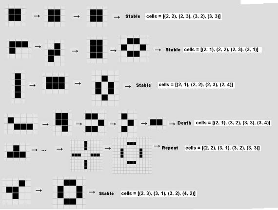
Figure 10-12. Additional starting patterns

There are a series of patterns that are dynamic, which means that they constantly move across the grid and repeat their patterns. Figure 10-13 shows the glider that moves around the grid and repeats its pattern every fourth generation.

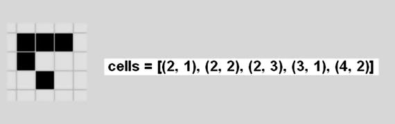
Figure 10-13. Glider pattern

A similar dynamic pattern is the lightweight spaceship, which is shown in Figure 10-14. It moves across the grid too.

Figure 10-14. Lightweight spaceship pattern

Conway discovered several patterns that took many generations to finally evolve and become both predictable and periodic. Incidentally, he made these discoveries without the aid of a computer. He called these patterns Methuselahs, after a man who was described in the Hebrew Bible to have lived to the age of 969 years. The first of these long-lived patterns is named F-pentomino, which is shown in Figure 10-15. It becomes stable after 1101 generations.

Figure 10-15. F-pentomino pattern

The Acorn pattern shown in Figure 10-16 is another example of a Methuselah that becomes stable and predictable after 5206 generations.

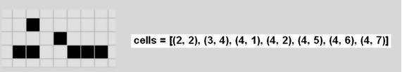
Figure 10-16. Acorn pattern

Readers who wish to experiment with more patterns can go to Alan Hensel’s webpage at radicaleye.com/lifepage/picgloss/picgloss.html, where he has compiled a fairly large list of other common patterns.

This completes the initial foray into cellular automata using Conway’s Game of Life as the tool. You should now be empowered to further experiment with this tool to gain more experience and confidence in this powerful AI topic. I also highly recommend Dr. Stephen Wolfram’s book A New Kind of Science (Wolfram Media, 2002), in which he examines the entire field of cellular automata using the Mathematica application, which he created. Incidentally, the Mathematica application is now freely provided with the latest Raspian distributions available from raspberrypi.org.