Boolean Algebra

Boolean algebra was created by George Boole in 1847. It is an algebra in which variable values are the truth values—true and false, often denoted as 1 and 0, respectively. There are a few very basic Boolean operations, which are frequently used in AI expressions. These operations are listed for variables A and B, as follows:

• A AND B

• A OR B

• NEGATE A

• NEGATE B

The expression A AND B may also be represented by A * B where the * symbol represents the AND’ing operation. It is not a true analog to the general multiplication symbol used in ordinary algebra, but it is close enough that most people use it interchangeably. Similarly, the expression A OR B can be represented by A + B, where the same observation holds true for the normal + symbol used in regular algebra. You will shortly see that there is a situation where 1 + 1 = 1 in Boolean algebra, but obviously is not true in non-Boolean algebra. The NEGATE or complement operation is unary, meaning it only uses one operand or variable; whereas AND and OR are binary, requiring two logical variables. The NEGATE operation has a formal symbol (¬), but it is not widely used in programs. Instead, a bar placed over the symbol is commonly used in most in logical expressions, which is the one that I use.

Table 2-1 shows the output resulting from various A and B inputs for the operations I just mentioned. Note that I use the variable C to represent the output.

Logical symbols can easily be arranged to form both simple and complex Boolean algebraic expressions. For instance, the AND’ing operation may be expressed as follows:

It should not be hard to realize that far more complex expressions can be created by using more than two variables and combined using these basic operations. However, the important point to understand is that eventually all expressions resolve to a true or false, 1 or 0 output.

There are also three secondary operations used in Boolean algebra:

• EXCLUSIVE OR

• MATERIAL IMPLICATION

• EQUIVALENCE

I use two of these three operations in inference discussion (material implication and equivalence), but I do not specifically call them out by their Boolean algebra names. In AI, there is a lot of overlap among the different subfields that go into overall AI technology; hence, it is not unusual to use concepts present in one subfield that uses a specific name that also exists in another subfield with a different name or reference. This differentiation should not bother you as long as you grasp the underlying concepts.

Inference

Inference is part of the reasoning process introduced in Chapter 1. This reasoning process consists of moving from an initial premise or statement of fact to a logical conclusion. Inference is ordinarily divided into three categories.

• Deduction: The derivation of a logical conclusion based on premises known or assumed to be true using the laws and rules of logic.

• Induction: Making a universal conclusion based upon specific premises.

• Abduction: Reduction of premises to the optimal explanation.

I use the inference deduction category for the following discussion, as it is the best fit for the topic of expert systems, which is introduced shortly.

There is a Latin phrase, modus ponens, which means “the way that affirms by affirming.” It represents the fundamental rule for deductive inference. Using logic terms, this rule may be stated as “P implies Q, and P is asserted to be true, so therefore Q must be true.” This rule dates to antiquity and has been used by logicians throughout the ages, up to and including the modern era. The rule may be broken into two sections. The first is a conditional claim that is traditionally stated in the form of if … then. The second part is the consequent of the conditional claim; that is, the logical statement following the then. The conditional claim for the general rule consists of two premises: that P implies Q and P is true. P is also known as the antecedent of the conditional claim. The consequent is obviously Q is true. The application of this simple modus ponens rule in AI is known as forward chaining, which is a key element in expert systems. I discuss it in the next section.

Expert Systems

An expert system is a computer program designed to use facts present in a specific problem domain. It then develops conclusions about those facts in a way analogous to a human expert reasoning with the same facts and reaching similar conclusions. Such a program or expert system would need access to all the facts in the domain, as well as be programmed with a set of rules that a human expert would follow regarding those facts and drawing conclusions from the same facts. Sometimes this expert system is known as a rules-based or knowledge-based system.

The first, large-scale expert system able to perform at a human-expert level was named MYCIN. It was used as an intelligent aide for doctors in their diagnosis of blood-borne infections. MYCIN incorporated about 450 rules. It was capable of creating correct diagnoses on a level comparable to an inexperienced doctor. The set of rules used in MYCIN was created based on interviews with a large number of experts in the field, who in turn relied on their own experiences and knowledge. To a large extent, the rules captured real-world data and knowledge beyond what was in medical textbooks and standard procedures. The rules used in MYCIN were in the same format I introduced earlier:

if (conditional claim) then (consequent)              

The following is an example:

if (bacteria in blood) then (septicemia)              

Incidentally, septicemia is a very serious blood-borne illness and must be treated immediately.

The conditional claim, which I will now simply shorten to the word condition may be complex by combining it with other conditions using the logical operators introduced in the Boolean algebra section. I will also use the word conclusion instead of consequent, because it is more commonly used in expert system design.

The following are some general formats for complex rules:

• if (condition1 and condition2) then (conclusion)

• if (condition1 or condition2) then (conclusion)

• if ((condition1 or condition2) and condition3) then (conclusion)

It is not hard to imagine that the MYCIN rules created were fairly complex, based upon the problem domain and all the variables or conditions present in that domain. The tools and techniques developed for MYCIN were later used in other expert systems.

Would there ever be a case where different conclusions could be reached given the same set of facts or conditions? The answer is definitely yes, and that is where conflict resolution enters the picture.

if (third down and long yardage to gain) then (pass play planned)                
if (blitz suspected) then (long yardage pass planned)                

if (blitz happens) then (execute long yardage pass play)                
if (blitz does not happen) then (execute screen pass play)                

Raspberry Pi Configuration

I connected to a Raspberry Pi running in a standalone setup using a headless or SSH connection. My client computer is a MacBook Pro, which I use for all my manuscript production. It also allowed me to easily capture screenshots of the terminal window controlling the Raspberry Pi. I find this connection type to be very efficient; it allows me full access to the Raspberry Pi and to all the files on my Mac. Everything displayed in the terminal window can be duplicated in a monitor connected directly to the Raspberry Pi, if this is the way you choose to run your own system. Of course, file manipulation on the Raspberry Pi has to be done through a command line, rather than through drag/drop/click—as is the case on a Mac.

Introduction to SWI Prolog

The AI language Prolog was initially created by mix of Scottish, French, and Canadian researchers from the 1960s to the early 1970s. It has been around a long time, considering how quickly modern computer languages are generated. Originally, the project’s purpose was to make deductions from French text extracted through automated means. This effort involved natural language processing, development of computer algorithms, and logical analysis. The name Prolog comes from a combination of three French words: PROgrammation en LOGique.

Prolog is considered a declarative programming language because it uses a set of facts and rules called a knowledge base. A Prolog user can address queries or questions to the knowledge base , which are knowns as goals. Prolog responds with an answer to the goal(s ) using logical deduction, as discussed in the inference section. Often, the answer is simply true or false, but it could be numerical, or even textual, depending upon how the goal was expressed.

Prolog is also considered a symbolic language, totally devoid of any connection to hardware or specific implementations. Prolog is often used by people with minimal computer knowledge, due to its level of abstraction. Most users do not need any prior computer programming experience to effectively use Prolog—at least at its most basic levels, as you will shortly experience.

From its start, Prolog was considered by the AI community as a shining example of what could be achieved by using symbols with AI. The language is essentially reasoning and logical processes, with the concepts of thinking and intelligence. While fairly simple from the outset, Prolog has become increasing complex as researchers add additional features and capabilities to the language. In my humble opinion, this has been both good and bad for the promotion of the language. Once quite simple and attractive to non-AI users, it has become quite complex and daunting to beginners in AI. However, do not fear: I keep things quite straightforward in the following Prolog demonstrations. However, be aware that you are only seeing the very tip of the “iceberg” when it comes to Prolog’s capabilities.

The computational power necessary to run Prolog has changed dramatically from the 1970s, when the equivalent of a supercomputer was necessary, compared to today, when a $35 single-board computer can easily and more quickly process Prolog queries.

Installing Prolog on a Raspberry Pi

The following instructions enable you to install a very capable and useful Prolog version, named SWI Prolog, on a Raspberry Pi. SWI is the acronym for social science informatics, as expressed in the Dutch language. SWI Prolog’s website is at www.swi-prolog.org . I urge you to take a look at this site because it contains a lot of useful tutorials and other key data.

To start the SWI Prolog installation, you first need to update your Raspian distribution. I assume that most readers are using the latest distribution, named Jessie, which was available from the Raspberry Pi Foundation at the time this book was written.

The first command you need to execute is the one that updates the Rasperry Pi Linux distribution:

sudo apt-get Update

The update should only take a few minutes to complete. Afterward, you are ready to install SWI Prolog. Enter the following:

sudo apt-get install swi-prolog

This command installs the SWI Prolog language along with all the required dependencies necessary for it to run on a Raspberry Pi. This installation takes several minutes or longer, depending on the Raspberry Pi model that you are using.

To test if you had a successful installation, simply enter the following:

swipl

You should see the following text appear on the monitor:

pi@raspberrypi:∼ $ swipl
Welcome to SWI-Prolog (Multi-threaded, 32 bits, Version 6.6.6)
Copyright (c) 1990-2013 University of Amsterdam, VU Amsterdam
SWI-Prolog comes with ABSOLUTELY NO WARRANTY. This is free software,
and you are welcome to redistribute it under certain conditions.
Please visit http://www.swi-prolog.org for details.

For help, use ?- help(Topic). or ?- apropos(Word).

?-

The prompt is ?-, which means that Prolog is awaiting your input. Assuming that you see this opening screen, you are set to start experimenting with Prolog, which is the subject of the next section.

Initial Prolog Demonstration

As I stated, you need a knowledge base to query Prolog. The knowledge base I use comes straight from a SWI Prolog tutorial that is located on their website. This knowledge base concerns the sun, planets, and a moon. The knowledge base is just a text file that should be put in the Raspberry Pi’s home directory. I created this text file using the default nano editor. I highly recommend that you also use nano; however, you certainly could use other text editors if you so desire. You should not use Microsoft Word or similar powerful word editors unless you ensure that all hidden formatting is excluded from the text file. Any hidden formatting causes the Prolog program to generate an error, so you would not be able to use that knowledge base.

The following is a listing of the knowledge base, which is named satellites.pl, and located in the pi directory.

%% a simple Prolog knowledge base

%% facts
orbits(earth, sun).
orbits(saturn, sun).
orbits(titan, saturn).

%% rules
satellite(X) :- orbits(X, _).
planet(X) :- orbits(X, sun).
moon(X) :- orbits(X, Y), planet(Y).

There are a few things that you should know about this knowledge base. Comments are started these symbols: %%. Comments are for human readers; they are ignored by the Prolog interpreter. Case counts in the file (meaning x and X) are not the same symbol. Facts and rules are always terminated with a period '.'.

You must use the consult command to force Prolog to use a knowledge base. In this situation, the command is with the name of the knowledge base without the .pl extension as the command argument:

?- consult(satellites).

This is a shorthand version of the consult command:

?- [satellites].

You can now start making queries, or setting goals, once the knowledge base is in place. The following is a simple query that asks if the Earth is a satellite of the sun:

?- satellite(earth).

The Prolog response is true because one of the facts in the knowledge base is that the Earth orbits the sun, and one of the rules is that a satellite is defined as any symbol that orbits the sun. Of course, the symbol used for this rule is the text “earth”. Figure 2-1 shows five queries that involve satellites, planets, and a moon.

Figure 2-1. Prolog knowledge base queries

Technically, moons also orbit the sun because their planets orbit the sun, but that can quickly become confusing, so it is left to the reader to ponder. Notice also that a halt. command is the last of the interactive Prolog entries shown in Figure 2-1. This command causes Prolog to stop and return control to the default operating system (OS) prompt.

It should be obvious that many additional facts can be added to the knowledge base to encompass more of the solar system. Additional rules can also be easily added to cover behaviors other than determining planet, satellite, and moon status. This flexibility is one of the inherent powers that Prolog possesses to handle more complex and comprehensive knowledge bases.

It should now also be obvious that through its knowledge bases, Prolog is a natural way to implement an expert system. One such system is thoroughly examined in the chapter devoted to expert systems. Now it is time to shift focus to discuss the approach fuzzy logic takes with AI.

Introduction to Fuzzy Logic

I start this section with the obvious point that there is nothing fuzzy or imprecise with the theory behind fuzzy logic (FL), which is so named because it goes well beyond a core concept in traditional logic that a statement is either true or false (also called a binary decision). In FL, a statement can be partially true or false. There can also be probabilities attached to a statement, such as There is a 60 percent chance that the statement is true. FL reflects reality in the sense that human beings not only make binary decisions but also decide things based on gradations. When you adjust the temperature in your shower, it is not just hot or cold but more likely warm or slightly cool. When driving, you likely adjust the speed of your car to the nominal traffic flow, which could easily be a little above the posted limit; you are not just speeding or stopped. These decisions—based on magnitude or gradations—are all around us. FL helps capture this decision making within AI. The following example should shed more light on what FL is and how it functions.

if (water temp is cold) then (turn on water heater)                
if (water temp is hot) then (turn off water heater)                

if (water is hot) then (turn on water heater)                

if (water is hot and kw-hr rate is high) then (turn on water heater)                

Problem Solving

Up until this point in the AI discussion, all the various questions/decisions regarding the problem domain have been carefully detailed in a comprehensive set of rules. That is not the case when it comes to the general topic of problem solving. Consider the classic example of knowing your starting and finishing points in your car’s GPS system. There are usually many ways to travel between two points, excluding the trivial case of going between two points on an isolated, desert highway. This is the type of problem that AI is very good at solving, often in a fast and efficient manner.

Let’s set up a scenario to examine the various facets of how to solve this problem. Consider a road trip between Boston and New York City. There are a variety of ways to make this trip. There are many paths between Boston and New York, because it is a heavily populated corridor with many towns and cities between the two locations. There will be some common-sense guidelines applied, including that any town or city on the path may be visited only once in a trip. It would not make much sense to repeatedly loop through a specific town or city during a trip. The key realistic points to consider in making the trip’s path selections are the costs that are manifested: travel time, path length, fuel costs, tolls and traffic density, which are actual or anticipated delays. These costs are often dependent because a longer path will increase fuel expenses, but not necessarily travel time because an alternate path could use a super highway, on which the car maintains a higher consistent speed, as compared to traveling through backroads and going through many small towns. But, a super highway can be congested, reducing overall speed, and there may even be tolls to add to the misery.

The first approach in determining the optimal path is called the breadth-first search.

Machine Learning

Machine learning was first defined in 1959 by MIT professor Arthur Samuel, a recognized pioneer in both computer science and artificial intelligence. Professor Samuel stated in part, “machine learning as a field of study that gives computers the ability to learn without being explicitly programmed.” What he was essentially driving at is that computers can be programmed with algorithms that can learn from input data and then make consequent predictions based on that same data. This means that learning algorithms can be completely divorced from any preprogrammed or static algorithms and be free to make data-driven decisions or predictions by building models based on the input data.

Machine learning is used in a many modern applications, including e-mail spam filters, optical character recognition (OCR) , textual search engines, computer vision, and more.

Implementing machine learning may be easier than you realize if you consider an expert system. In a traditional expert system, there are a series of rules generated by interviewing experts, which are then “fired” using input conditions. What if a machine could take one or more of those rules and slightly modify them, and subsequently try to use the conclusions generated by the modified rules? If the new modified rules improved upon the final conclusion, then they would be retained and perhaps awarded with somewhat higher priorities than older rules, similar to what is done with conflict resolution. On the other hand, if the conclusions reached using the modified rules were less optimal, then they would be rejected and replaced with additional new rule modifications. If this was a continual process, could it not be said that the computer is indeed learning? Answering this type of question has been somewhat of a contentious area within the AI community.

There are a variety of ways to implement machine learning. I discuss a few of them in the following sections. However, I think it would be prudent to review some fundamental concepts (prediction and classification) regarding learning, as it will be applied in this area.

Prediction

Prediction is how you determine a new output value using specific input with a model that relates the output to the input. Perhaps the simplest predictor is a sloped straight line going through the origin of an x-y graph. This is easily modeled by the following equation and is shown graphically in Figure 2-2.

Figure 2-2. Graph of

There are a several hidden constraints using this predictor. First, is the allowed range of input values. In Figure 2-2, there are five output values plotted that match the five corresponding input values ranging between 0 and 10. Normally, you could assume that the input values were not restricted to this same range, but models in the real world could have restrictions, such as only non-negative numbers are allowed. In addition, while the equation is linear within the plotted zone, there is no guarantee that a real-world model wouldn’t become non-linear if input values exceeded a certain value.

As you have probably determined from the brief introduction, useful prediction is only as good as the model employed in the prediction. Realistic models are typically much more complex than a simple straight-line equation, because modeling real-world behavior is a complex matter. Now it is time to consider classification, which is as equally important as prediction.

Classification

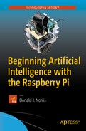
I begin the classification discussion by stating a hypothetical situation where it is import to classify a select species of mushroom. Note, the mushrooms discussed are pure fiction, so any mycologists (fungi experts) in my readership need not respond. Assume there are two mushroom types: one delicious and non-poisonous, and the other poisonous and obviously inedible. They look almost identical; however, the edible variety is larger and less dense, whereas the poisonous variety is smaller and denser. There are two parameters or input values used to classify these mushroom types: weight in grams and the crown (or cap) circumference in millimetres (mm). Density is a derived parameter, which can be determined, if needed, from the two basic measurements of weight and circumference. Figure 2-3 is an x-y scatter plot of a selection of both mushroom types.

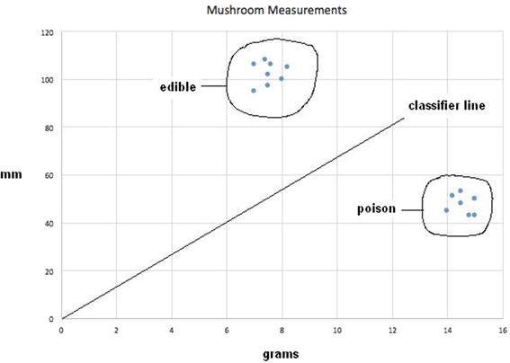
Figure 2-3. Mushroom scatter plot

In Figure 2-3, I encircled all the data points for both mushroom types, and I placed a sloped dividing line, labeled classification line. This line clearly divides the two groups, as you can easily see, but the problem remains as to how to best analytically determine the diving line. The line equation is precisely the same form shown in Figure 2-1, with a generalized form of

where m is the slope. Let’s try m = 2 for an initial value and see what happens. Figure 2-4 shows the result.

Figure 2-4. Scatter plot with classification line y = 2x

Clearly, this is not a satisfactory result, as both data point clusters are on the same side of the line, which proves that this particular choice for m cannot serve as a useful classifier. What is needed is a precise way of determining m other than using a blind manual trial-and-error approach. This approach is the start of a machine learning process.

I first need to establish what is known as a training data set, which will be used to assess how well the classifier function works. This data is simply a data point from each cluster, as shown in Table 2-3.

Table 2-3. Training Data

Data Point #	Grams (x)	mm (y)	Mushroom type
1	15	50	poisonous
2	8	100	edible

Substituting the x value for data point 1 into the equation yields a value of 30 for y instead of 100, which is the true or target value. The difference of +20 is known as the error value. It must be minimized to achieve a workable classifier. Increasing the classifier line slope is the only way to minimize the error. Let's use the symbol ∆ to represent a change in the slope, € for the error, and y _t for the desired target value. The error thus becomes

Expand the preceding equation with the assumption that ∆ assumes a value that allows y _t to be reached yields the following:

Expanding and collecting terms yields the following:

The very simple final expression for the error term is simply the Δ value times the input value, which makes complete sense if you reflect on it for a while. Rearranging the last equation and solving for Δ yields

Plugging in the initial trial values yields a Δ value of

The new value for m is now 1.3333 + 2, or 1.3333, and the revised classifier line equation is consequently

Plugging in the previous value for the x training value, or 15, now yields the desired target value of 50. Figure 2-5 shows the revised classifier line on the scatter plot.

Figure 2-5. Revised classifier line y = 3.3333x

Further Classification

While the revised classifier line has improved the classification somewhat there are still poisonous mushrooms data points either on or above the line, which still makes this classifier line unsatisfactory.

Now, let’s use data point number 2 with this revised classifier line and see what results. Using the value x = 8 yields a y value of 26.664. Now, the actual y data point value is 100, which means that € = 100 – 26.664 = 73.336. A newly revised m value can be calculated as follows:

Plugging in the training value x, which is 8, now yields the desired target value of 50. Figure 2-6 shows the newly revised classifier line on the scatter plot.

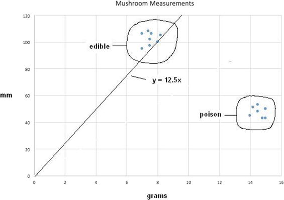
Figure 2-6. Revised classifier line y = 12.5x

While this newly revised classifier line does separate all the edible mushrooms from the poisonous ones, it is unsatisfactory: there could still be some edible mushrooms falsely rejected because they fell slightly below the line. Now there exists a larger problem, however, because all the training points have been exhausted. If I went back and reused the previous point number 1, it would return to the classifier line. This is because the procedure does not consider the effects of any previous data points; that is, there is no memory. A way around this is to introduce the concept of a learning rate that moderates the revisions so that they do not jump to the extremes, which is what is happening at present.

The standard symbol used in AI for learning rate is η (the Greek letter Eta). The learning rate is a simple multiplier used in the equation for Δ:

Setting η = 0.5 is a reasonable start, if only one-half the update is applied. For the initial data point, the new Δ = 0.5 * 1.333 = 0.667. The new classifier line is therefore y = 2.667x. I am not going to show the scatter plot line for this change, but suffice it to say, it is slightly worse than the original revision. That’s OK because the next revision should be considerably better.

For data point 2, the new classifier line is y = 6.25x, using the new η learning rate. Figure 2-7 shows the resulting scatter plot for this new classifier line.

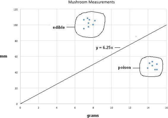
Figure 2-7. Revised classifier line y = 6.25x

Figure 2-7 reveals an excellent classifier line that properly separates the two mushroom types, minimizing the likelihood of a false classification.

It is now time to introduce the very fundamental concept of a neural network, which is essential for implementing practical machine learning.

Neural Networks

The concept of neural networks can be traced back to a 1943 research article by McCulloch and Pitts, which focused on neurocomputing. I first mentioned these pioneering researchers in Chapter 1. This article shows that simple neural networks could, in principle, compute any arithmetic or logical function. To understand a neural network, you must understand the key element in a biological neural network, which is the neuron. Figure 2-8 is a diagram of a human neuron.

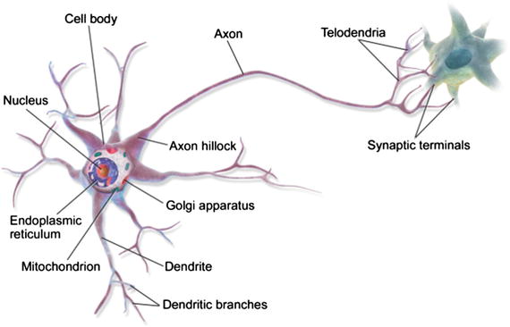
Figure 2-8. Diagram of a human neuron (Source: Wikipedia)

Figure 2-9 is a sketch of pigeon brain neurons , created in 1899 by Spanish neuroscientist Santiago Ramón y Cajal. Dendrites and terminals are clearly shown in the figure.

Figure 2-9. Pigeon brain neurons sketch (Source: Wikipedia)

The question now becomes Why is the human brain so much more capable of successfully undertaking intelligent tasks when compared to modern computers? One answer is that a mature human brain is estimated to have over 100 billion neurons. The precise functioning is still unknown. To get an idea of the inherent capabilities of such a large number of neurons, you can simply consider the capabilities of a simple earthworm, which has only 302 neurons, yet is still capable of doing tasks that would baffle large-scale computers.

Examining how a single neuron functions helps explain how a network of them can be created to solve AI problems. The output signal from a neuron can either cause an excitation or an inhibition to a neuron immediately connected to it. When a neuron sends an excitation signal to the connected neuron, it is added to all the other inputs that neuron is concurrently receiving, and when the combined excitation of all the inputs reaches a preset level or threshold, that neuron will fire. The firing does not depend on the level of any given input; it only matters that the threshold be exceeded to initiate a firing. Figure 2-10 shows a time trace of a typical neuron electrical signal.

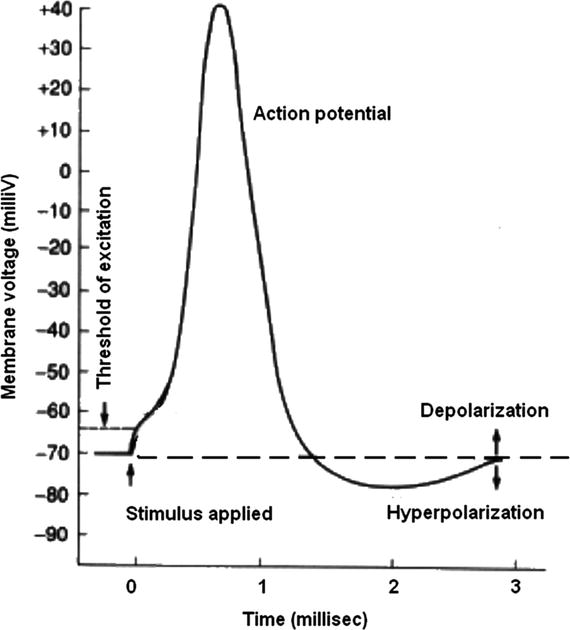
Figure 2-10. Firing neuron time trace

As you can see in Figure 2-10, the peak voltage is only 40 millivolts and total pulse time duration is approximately 3 milliseconds (ms). Most neurons have one axon, so the delay between stimulus input and excitation output in a given neuron is only 3 ms. It is interesting to try to relate this to human reaction time. The fastest human reaction time ever verified is 101 ms, with the average being approximately 215 ms. This is the total time that it takes to progress from a sensory input, such as sight, to a motor actuation, such as a mouse click. Assume that it takes 10 ms to send a signal from the eyes to the appropriate neurons in the brain; perhaps 20 ms to send a nerve signal from the neurons controlling finger-muscle action and 40 ms for muscle activation itself. This leaves about 145 ms for total brain-processing time. That time duration limits the longest chain of neurons to about 14 to 15 in length. That number implies there must be a huge number of short parallel neuron chains interoperating to accomplish the tasks of interpreting a visual signal, recalling the appropriate action to take, and then sending nerve control signals to the fingers to do a mouse click. And all of these tasks are done dynamically while still doing the background autonomic things necessary to stay alive.

The neuron’s excitation action can be roughly modeled by using a step function, as shown in Figure 2-11.

Figure 2-11. Step function

In nature, nothing is ever as sharp and defined as a step function, especially for biological functions. AI researchers have adopted the sigmoid function as more realistically modeling the neuron threshold function. Figure 2-12 shows the sigmoid function.

Figure 2-12. Sigmoid function

The sigmoid function analytic expression is

, where e = math constant 2.71828…

When x = 0, then y = 0.5, which is the y axis intercept for the sigmoid function. This function is used as the threshold function for our neuron model. Consider Figure 2-13 a very basic neuron model with three inputs (x1, x2, and x3) and one output (y).

Figure 2-13. Basic three-input neuron model

The basic model is useful, but it is not the complete answer because neurons must be connected to a network to function as a learning entity. Figure 2-14 shows a simple neural network made up of three neuron layers, labeled input, hidden, and output, respectively.

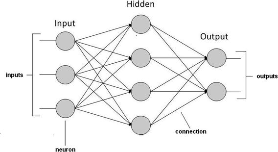
Figure 2-14. Example neural network

The next obvious question is How does this network learn? The easiest way is to adjust the weights of the connections. This means adjusting the amplitude or strength from an output to an input. Thus, a high weight means a given connection is emphasized more, whereas a low weight is de-emphasized. Figure 2-15 shows weights assigned to each of the neuron, or node, connections. They are shown as w_n,m, where n is the source node number and m is the destination node number.

Figure 2-15. Neural network with weighted interconnections

At this point, I defer any further discussion until the neural network chapter, in which I assign actual weights and demonstrate an actual learning system. The primary purpose of the discussion to this point is to prepare you for the neural network implementation.

Shallow Learning vs. Deep Learning

You may have heard the terms shallow and deep applied to machine learning. The term shallow seems to imply that somewhat trivial and lightweight learning is going on, whereas deep implies the opposite. In actuality, shallow learning and deep learning are only subjective adjectives applied to neural networks, based upon the number of layers implemented in the network. There really isn’t a formal definition separating shallow from deep learning, because the effectiveness of a particular neural network is determined by many factors, one of which is the number of layers in the network. The point in stating this is because I am not really worried about whether a particular neural network is classified as shallow or deep, but I am concerned about its effectiveness in performing at the desired requirements and standards.

Evolutionary Computing

There is a rapidly evolving AI field called evolutionary computing. It is inspired by the theory of biological evolution, but uses algorithms grounded on population-based trial-and-error problem solvers. In turn, these problem solvers use metaheuristic techniques, meaning they rely on statistical and probabilistic approaches rather than strict deterministic, analytical techniques. In broad terms, an evolutionary computing problem starts with an initial set of candidate solutions, which are subsequently tested for optimality. If they are found to be suboptimal, the solutions are altered by only a small random amount and then retested. Every new generation of candidate solutions is improved by removing the less desired solutions determined from the previous generation. A biological analog is when a population is subjected to natural selection and mutations. This results in the population gradually evolving to increase overall fitness to meet environmental conditions. For evolutionary computing, the analogous process is to optimize the algorithm’s pre-selected fitness function. In fact, evolutionary computation is sometimes used by researchers in evolutionary biology for experimental procedures to study common processes.

Evolutionary computing can be used in other AI areas. If you recall, I alluded to an evolutionary computing approach when I stated that a machine could take one or more of those rules and slightly modify them, and subsequently try to use the conclusions generated by the modified rules. It would likely be a difficult but solvable problem to create a candidate set of expert rules subjected to the evolutionary screening process.

A very popular subset of evolutionary computing is known as genetic algorithms, which I briefly introduce in the next section.

Summary

The primary purpose of this chapter was to introduce and discuss some basic AI concepts that will be demonstrated in the project chapters. I began with a brief overview of Boolean logic and associated logical operations, as these are frequently used in AI expressions. The remainder of the chapter provided an overview of the following:

• Inference, expert systems, and conflict resolution as it pertains to implementing an expert system

• The installation of SWI Prolog on a Raspberry Pi

• A Prolog demo, which is my program of choice to implement an expert system when required for a project

• A simple example of fuzzy logic to help clarify the underlying concepts

• A series of sections on machine learning

• Neural networks (NN), which are modeled after biological brain neurons

• Evolutionary computing that features genetic algorithms