Parts List

For the last demonstration, you need the parts listed in Table 5-1.

Software Installation

First, you need Python 2.7, which should already be installed as part of the Jessie Linux distribution. You also need the numpy, scipy, matplotlib, and skfuzzy packages, which implement FL with Python and the plotting functions that create the visualizations.

Enter the following commands at the command line to install the numpy, scipy, and matplotlib software:

sudo apt-get update
sudo apt-get install python-numpy

sudo apt-get install python-scipy
sudo apt-get install python-matplotlib

The skfuzzy software is somewhat more complex to install. You need to clone the software from the GitHub website; however, you need the Git application to do this. So install Git by entering this command:

sudo apt-get install git

Once Git is installed, you then need to clone the software by using this command:

sudo git clone https://github.com/scikit-fuzzy/scikit-fuzzy.git

The cloning operation automatically unzips all the skfuzzy software into a new subdirectory named scikit-fuzzy, located in the home directory. Enter the following commands to set up skfuzzy:

cd scikit-fuzzy
sudo python setup.py install

You will see a lot of dialog scroll by as the skfuzzy installation is in progress. After this installation, you should be all set to execute fuzzy Python scripts.

Basic FLS

Figure 5-1 shows all four of the principal components that make up a basic FLS.

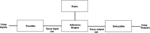
Figure 5-1. Block diagram for a basic FLS

These are the principal FLS components :

• Fuzzifier: The process in which a crisp set of input data is collected and converted to a fuzzy set using fuzzy linguistic variables, fuzzy linguistic terms, and membership functions.

• Rules: The expert knowledge collected and codified into the inference engine.

• Inference engine: Inferences are generated based upon a set of rules applied to the input fuzzy set.

• Defuzzifier: Crisp outputs are created based on the fuzzy set output from the inference engine.

Figure 5-1 may also be expressed as a series of steps or a logical algorithm that implements the FL process. I use this generic algorithm, shown in Table 5-2, to implement all of the chapter’s FLS demonstration projects.

Initialization: Define Linguistic Variables and Terms

The linguistic variables that I just introduced are values that represent the inputs and outputs of the system. They are not typically numerical values but instead are usually words, or even sentences, from a natural language, such as English. Linguistic variables are also decomposed into a set of linguistic terms.

Demo 5-1: Using FL to Calculate a Tip

In a tipping scenario , there are a number of input variables that go into the decision about how much to tip the server after completing a restaurant meal. Let us consider two primary inputs: food quality and service quality.

I do realize that many people, when determining a tip, differentiate the quality of the food from the quality of the service because the server has no control over food quality or preparation other than ensuring that the meal is still hot when served at the table. For this demonstration, however, I consider food quality as a valid input.

The only output variable is the tip amount, which is a percentage of the total bill.

Now, it is important to develop some linguistic terms that are appropriate to this situation.

Perhaps the easiest and most obvious way to classify food quality is to use the following terms:

• great

• decent

• bad

Likewise, classifying service quality uses these terms:

• amazing

• acceptable

• poor

The tip amount is also subject to fuzzy linguistic terms. These are the terms used for the tip amount:

• low

• medium

• high

There must be a numerical scale for users to rate both the service quality and the food quality. A scale of 0 to 10 is fine for most people, where 0 is the worst and 10 is the best. The tip output must also have a numerical scale. This is set at 0 to 26 to represent a suitable scale for normal tipping percentages. All of these numerical scales represent the crisp or non-fuzzy inputs or outputs to the membership functions, which are discussed in the next section.

Initialization: Construct Membership Functions

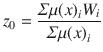
Membership functions are used in both FL fuzzification and defuzzification steps. These functions map non-fuzzy input values to fuzzy linguistic variables for fuzzification, and map fuzzy variables to non-fuzzy output values for defuzzification. Essentially, a membership function quantifies linguistic terms. Figure 5-2 shows the food quality membership function.

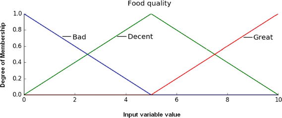
Figure 5-2. Food quality membership function

Figure 5-3 shows the service quality membership function.

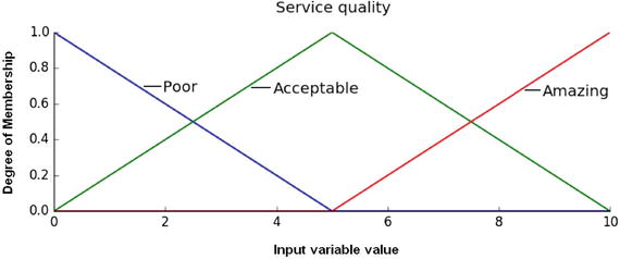
Figure 5-3. Service quality membership function

Finally, Figure 5-4 shows the tip amount membership function.

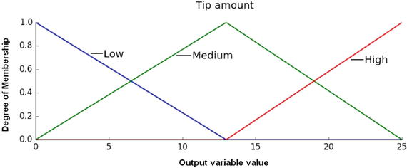
Figure 5-4. Tip amount membership function

I chose to use triangular shapes for the decent, acceptable, and medium linguistic terms. I use open-ended trapezoid shapes for the extremis bad, great, poor, amazing, low, and high terms. There are shapes other than triangular that are commonly used for membership functions, including

• Gaussian

• trapezoidal

• singleton

• piecewise linear

• sinusoidal

• exponential

The selection of an appropriate membership function shape is often based on the user’s experience. I sometimes use the following analogy to help people understand membership functions. Suppose that you interviewed a large group of people on their preferences in determining an appropriate amount to tip, given the quality of the food and the service. As most of my readers understand, the resulting distribution of tip values is Gaussian, or normal in shape, which is the likely outcome of randomly interviewing large numbers of people. Any point on a Gaussian curve is the group probability for the corresponding measure of food and service quality. It is perfectly possible to use a Gaussian distribution shape as the membership function, as shown in Figure 5-5.

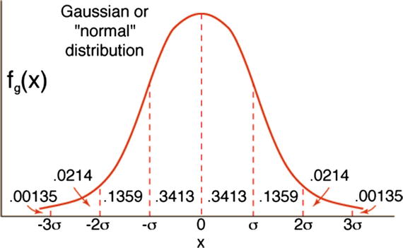
Figure 5-5. Gaussian membership function

The only problem with using this shape is that you are now dealing with the underlying mathematics behind the Gaussian curve, which rapidly becomes messy and cumbersome when trying to use it in an FL application. A normalized Gaussian equation is of the following form:

where a, b, and c are generalized parameters

The Gaussian curve is mostly likely a better model of human behavior and choice for this example, but using it is not worth the effort, as the AI concepts can be well understood using the much simpler triangular shape for the membership curves.

# Visualize the membership functions
fig, (ax0, ax1, ax2) = plt.subplots(nrows=3, figsize=(8, 9))
                                                                                                        
ax0.plot(x_qual, qual_lo, 'b', linewidth=1.5, label='Bad')
ax0.plot(x_qual, qual_md, 'g', linewidth=1.5, label='Decent')
ax0.plot(x_qual, qual_hi, 'r', linewidth=1.5, label='Great')
ax0.set_title('Food quality')
ax0.legend()

ax1.plot(x_serv, serv_lo, 'b', linewidth=1.5, label='Poor')
ax1.plot(x_serv, serv_md, 'g', linewidth=1.5, label='Acceptable')
ax1.plot(x_serv, serv_hi, 'r', linewidth=1.5, label='Amazing')
ax1.set_title('Service quality')
ax1.legend()

ax2.plot(x_tip, tip_lo, 'b', linewidth=1.5, label='Low')
ax2.plot(x_tip, tip_md, 'g', linewidth=1.5, label='Medium')
ax2.plot(x_tip, tip_hi, 'r', linewidth=1.5, label='High')
ax2.set_title('Tip amount')
ax2.legend()

# Turn off top/right axes
for ax in (ax0, ax1, ax2):
    ax.spines['top'].set_visible(False)
    ax.spines['right'].set_visible(False)
    ax.get_xaxis().tick_bottom()
    ax.get_yaxis().tick_left()

plt.tight_layout()

Initialization: Build Rule Set

An FLS also requires an expert system to generate the appropriate control actions based upon the fuzzified input variables. This expert system is of the form if <condition> then <conclusion>, which was discussed in Chapter 2. The following are the rules implemented for this FLS demonstration:

• if the food is bad or the service is poor, then the tip will be low

• if the service is acceptable, then the tip will be medium

• if the food is great or the service is amazing, then the tip will be high

These three rules apply to both the input variables and the output variable. I discuss how the rules are applied after the fuzzification section discussion, which is next. Fuzzification is step 4 in the FLS algorithm.

Fuzzification : Convert crisp input data a into fuzzy set using membership functions.

The membership function shapes and the rules for generating an appropriate tip percentage are set. The next thing is to show you how to fuzzify the crisp food and service ratings. The procedure is exactly the same for each of these crisp variables, because I chose the same membership function shapes for each one. That choice can vary and it is often common to have distinct and separate member functions in an FLS for different crisp variables.

The word fuzzification refers to the action of converting a crisp set of input data to a fuzzy set using fuzzy linguistic variables and terms along with membership functions. The actual fuzzification takes place in a set of functions that depend upon the following code segment, which creates the input and output variable ranges and the membership functions:

import numpy as np
import skfuzzy as fuzz
import matplotlib.pyplot as plt

# Generate universe variables
#   * food quality and service on subjective ranges, 0 to 10
#   * tip has a range of 0 to 25 in units of percentage points
x_qual = np.arange(0, 11, 1)
x_serv = np.arange(0, 11, 1)
x_tip  = np.arange(0, 26, 1)

# Generate fuzzy membership functions
qual_lo = fuzz.trimf(x_qual, [0, 0, 5])
qual_md = fuzz.trimf(x_qual, [0, 5, 10])
qual_hi = fuzz.trimf(x_qual, [5, 10, 10])
serv_lo = fuzz.trimf(x_serv, [0, 0, 5])
serv_md = fuzz.trimf(x_serv, [0, 5, 10])
serv_hi = fuzz.trimf(x_serv, [5, 10, 10])
tip_lo  = fuzz.trimf(x_tip,  [0, 0, 13])
tip_md  = fuzz.trimf(x_tip,  [0, 13, 25])
tip_hi  = fuzz.trimf(x_tip,  [13, 25, 25])

To test the algorithm, let’s assume that the food quality was valued at 6.5 and the service at 9.8. The following code segment calculates the six degrees of membership for each input variable and membership function:

qual_level_lo = fuzz.interp_membership(x_qual, qual_lo, 6.5)
qual_level_md = fuzz.interp_membership(x_qual, qual_md, 6.5)
qual_level_hi = fuzz.interp_membership(x_qual, qual_hi, 6.5)

serv_level_lo = fuzz.interp_membership(x_serv, serv_lo, 9.8)
serv_level_md = fuzz.interp_membership(x_serv, serv_md, 9.8)
serv_level_hi = fuzz.interp_membership(x_serv, serv_hi, 9.8)

The fuzz.interp_membership(a, b, c) function is part of the skfuzzy library that you installed earlier. This is an interpolation function that uses the membership function range (a) and linear shape (b) along with the crisp input value (c) to calculate the degree of membership for that particular group.

It is time to apply the rules once the degree of membership values has been determined. This is step 5 of the algorithm or inference.

Inference: Evaluate Fuzzy Set According to Rule Set

Applying the if … then inferential rules is rather easy because all you must do is focus on how the linguistic terms are related. For instance, this is rule 1:

• if the food is bad or the service is poor, then the tip will be low

The conjunction between the bad and poor linguistic terms is the or operator. In fuzzy logic, using an or operator is equivalent to selecting the maximum of the two membership values representing the respective linguistic terms. If you refer back to Figures 5-2 and 5-3, you quickly see that there are no intersections with either the bad and poor membership functions for the assumed crisp input variable values, so the result of applying this rule must be 0. Connecting the combined bad and poor linguistic terms to the low tip membership function is trivial because the value is still 0 more than the universe of applicable values.

Applying rule 2 is a bit different. This is rule 2:

If the service is acceptable, then the tip will be medium.

In this case, only the service membership function is considered for input. Referring back to Figure 5-3, you see that applying a crisp input variable value of 9.8 to the acceptable membership group results in a degree of membership of approximately 0.02. The and operator is then applied to the acceptable service and medium tip membership functions, which results in the minimum operation being applied to both membership functions. This minimum operation effectively “flattops” the membership functions, resulting in a new shape, as shown in Figure 5-6. Note also that the input range has been expanded to accommodate the tip value range, which is 2.5 times the input service range. Notice also that the slopes of the lines at the ends of the membership function are lessened due to the expanded x-axis scale.

Figure 5-6. Service and tip membership functions after rule 2 is applied

Rule 3 is the last to be applied:

If the food is great or the service is amazing, then the tip will be high.

The or operation is applied for rule 3, just as it was for rule 1. But in this case, there are definite intersections with the great and amazing membership functions. Figure 5-7 shows both the food and the service membership functions after being flattop but before being combined.

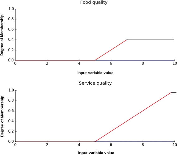
Figure 5-7. Flattop food and service membership functions

Figure 5-8 shows the great, amazing, and high membership functions combined. It should not be a big surprise that the shape is roughly the same as the unmodified membership functions because the or operation commands the maximum value and the two unmodified membership shapes are exactly the same. The shape also remains unchanged after the combined membership function is “anded” with the high tip membership function, although the range of x-axis values changes to 0 to 25 to accommodate the tip range, as done with the previous rule, and the flattop region expands a bit due to the x-axis expansion.

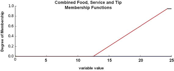
Figure 5-8. Combined great, amazing, and high membership functions

The following code segment applies the rules and combines the membership functions:

# Apply rule 1
# The 'or' operator means to take the maximum by using the 'np.max' function

active_rule1 = np.fmax(qual_level_lo, serv_level_lo)

# Next, flattop the corresponding output
# Combine with low tip membership function using `np.fmin`

tip_activation_lo = np.fmin(active_rule1, tip_lo)  # Removed entirely to 0

# Rule 2  connects acceptable service to medium tipping
# No flat topping needed as there is only one input membership function
# However, the tip membership must be combined using an 'and' or 'np.fmin' function

tip_activation_md = np.fmin(serv_level_md, tip_md)

# Rule 3 connects amazing service or great food with high tipping

active_rule3 = np.fmax(qual_level_hi, serv_level_hi)
tip_activation_hi = np.fmin(active_rule3, tip_hi)

At this point, all the rules have been applied to the output membership functions. It now remains to combine them all. In FL terminology, this is known as aggregation, which is step 6 in the FLS algorithm.

Aggregation: Combine Results from Each Rule Evaluation

Aggregation is normally done using the maximum operator. The following statement does the aggregation:

# Aggregate all three output membership functions together

aggregated = np.fmax(tip_activation_lo, np.fmax(tip_activation_md, tip_activation_hi))

Figure 5-9 shows the final combined membership functions after the aggregation is complete.

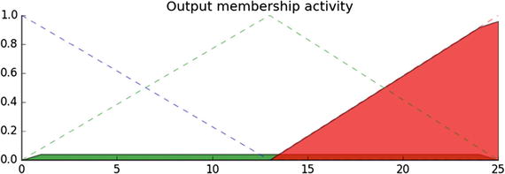
Figure 5-9. Membership functions after aggregation

There is only one more step in the FLS algorithm: defuzzification.

Defuzzification: Convert Fuzzy Set to Crisp Output Values

Defuzzification is the process where we return from the fuzzy world to the real world and create an output that can be acted upon, which in this case is a tip percentage. There are a variety of mathematical techniques available for defuzzification, including

• centroid

• bisector

• mean

• smallest of maximum

• largest of maximum

• weighted average

Figure 5-10 demonstrates how values for each method are chosen using an arbitrary aggregation membership function.

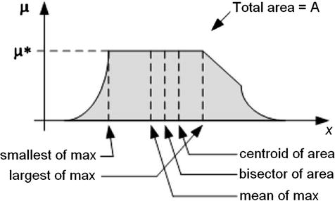
Figure 5-10. Various defuzzification methods

Centroid defuzzification is the most commonly used method because it is very accurate. It calculates the center of the area under the curve of membership function. This can require significant computational processing for complex membership functions. The centroid equation is

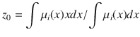
where z ₀ is the defuzzified output, μ _i represents a membership function, and x is the output variable.

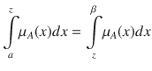
Bisector defuzzification uses vertical lines that divide the area under the membership curve into two equal areas:

The mean of maximum (MOM) defuzzification method uses the average value of the aggregated membership function outputs.

The smallest of maximum defuzzification method uses the minimum value of the aggregated membership function outputs.

The largest of maximum defuzzification method uses the maximum value of the aggregated membership function outputs.

The weighted average defuzzification method calculates the weighted sum of each fuzzy set. The crisp value is set according to the weighted values and the degree of membership for fuzzy output, as determined by the following formula:

μ _i is the degree of membership in output singleton i and W _i is the fuzzy output weight value for the output singleton i.

Next, I discuss how the centroid method is implemented for this project. The following code snippet calculates the centroid defuzzification value:

# Calculate defuzzified result
tip = fuzz.defuzz(x_tip, aggregated, 'centroid')

# This value is needed for the plot
tip_activation = fuzz.interp_membership(x_tip, aggregated, tip)

This section completes the tipping fuzzy logic project. All that’s left to do is load and run the following code, which is named tipping.py . Enter the following to run the program:

sudo python tipping.py

You need to close each plot after it appears to go on to the next plot.

tipping.py listing

import numpy as np
import skfuzzy as fuzz
import matplotlib.pyplot as plt

# Generate universe variables
#   * Quality and service on subjective ranges [0, 10]
#   * Tip has a range of [0, 25] in units of percentage points
x_qual = np.arange(0, 11, 1)
x_serv = np.arange(0, 11, 1)
x_tip  = np.arange(0, 26, 1)
                                                                          
# Generate fuzzy membership functions
qual_lo = fuzz.trimf(x_qual, [0, 0, 5])
qual_md = fuzz.trimf(x_qual, [0, 5, 10])
qual_hi = fuzz.trimf(x_qual, [5, 10, 10])
serv_lo = fuzz.trimf(x_serv, [0, 0, 5])
serv_md = fuzz.trimf(x_serv, [0, 5, 10])
serv_hi = fuzz.trimf(x_serv, [5, 10, 10])
tip_lo = fuzz.trimf(x_tip, [0, 0, 13])
tip_md = fuzz.trimf(x_tip, [0, 13, 25])
tip_hi = fuzz.trimf(x_tip, [13, 25, 25])

# Visualize these universes and membership functions
fig, (ax0, ax1, ax2) = plt.subplots(nrows=3, figsize=(8, 9))

ax0.plot(x_qual, qual_lo, 'b', linewidth=1.5, label='Bad')
ax0.plot(x_qual, qual_md, 'g', linewidth=1.5, label='Decent')
ax0.plot(x_qual, qual_hi, 'r', linewidth=1.5, label='Great')
ax0.set_title('Food quality')
ax0.legend()

ax1.plot(x_serv, serv_lo, 'b', linewidth=1.5, label='Poor')
ax1.plot(x_serv, serv_md, 'g', linewidth=1.5, label='Acceptable')
ax1.plot(x_serv, serv_hi, 'r', linewidth=1.5, label='Amazing')
ax1.set_title('Service quality')
ax1.legend()

ax2.plot(x_tip, tip_lo, 'b', linewidth=1.5, label='Low')
ax2.plot(x_tip, tip_md, 'g', linewidth=1.5, label='Medium')
ax2.plot(x_tip, tip_hi, 'r', linewidth=1.5, label='High')                                                                      
ax2.set_title('Tip amount')
ax2.legend()

# Turn off top/right axes
for ax in (ax0, ax1, ax2):
    ax.spines['top'].set_visible(False)
    ax.spines['right'].set_visible(False)
    ax.get_xaxis().tick_bottom()
    ax.get_yaxis().tick_left()

plt.tight_layout()
plt.show()

# Calculate degrees of membership
# The exact values 6.5 and 9.8 do not exist on our universes
# Use fuzz.interp_membership to determine values

qual_level_lo = fuzz.interp_membership(x_qual, qual_lo, 6.5)
qual_level_md = fuzz.interp_membership(x_qual, qual_md, 6.5)
qual_level_hi = fuzz.interp_membership(x_qual, qual_hi, 6.5)

serv_level_lo = fuzz.interp_membership(x_serv, serv_lo, 9.8)
serv_level_md = fuzz.interp_membership(x_serv, serv_md, 9.8)
serv_level_hi = fuzz.interp_membership(x_serv, serv_hi, 9.8)

# Apply the rules, Rule 1 concerns bad food OR service.
# The OR operator means we take the maximum of these two.

active_rule1 = np.fmax(qual_level_lo, serv_level_lo)

# Now we apply this by clipping the top off the corresponding output
# membership function with `np.fmin`

tip_activation_lo = np.fmin(active_rule1, tip_lo)  # removed entirely to 0
                                                                          
# Rule 2 is a straight if ... then construction
# if acceptable service then medium tipping. This is an AND operator
# We take the minimum for an AND operator

tip_activation_md = np.fmin(serv_level_md, tip_md)

# For rule 3 we connect high service OR high food with high tipping
active_rule3 = np.fmax(qual_level_hi, serv_level_hi)
tip_activation_hi = np.fmin(active_rule3, tip_hi)
tip0 = np.zeros_like(x_tip)

# Visualize these rule applications

fig, ax0 = plt.subplots(figsize=(8, 3))
ax0.fill_between(x_tip, tip0, tip_activation_lo, facecolor='b', alpha=0.7)
ax0.plot(x_tip, tip_lo, 'b', linewidth=0.5, linestyle='--', )
ax0.fill_between(x_tip, tip0, tip_activation_md, facecolor='g', alpha=0.7)
ax0.plot(x_tip, tip_md, 'g', linewidth=0.5, linestyle='--')
ax0.fill_between(x_tip, tip0, tip_activation_hi, facecolor='r', alpha=0.7)
ax0.plot(x_tip, tip_hi, 'r', linewidth=0.5, linestyle='--')
ax0.set_title('Output membership activity')

# Turn off top/right axes

for ax in (ax0,):
    ax.spines['top'].set_visible(False)
    ax.spines['right'].set_visible(False)
    ax.get_xaxis().tick_bottom()
    ax.get_yaxis().tick_left()

plt.tight_layout()
plt.show()
                                                                          
# Aggregate all three output membership functions together
# This aggregation uses OR operators, hence the maximum is found

aggregated = np.fmax(tip_activation_lo, np.fmax(tip_activation_md, tip_activation_hi))

# Calculate defuzzified result using the method of centroids
tip = fuzz.defuzz(x_tip, aggregated, 'centroid')

# display the tip percentage on the console
print tip

# Value needed for the next plot
tip_activation = fuzz.interp_membership(x_tip, aggregated, tip)

# Visualize the final results
fig, ax0 = plt.subplots(figsize=(8, 3))

ax0.plot(x_tip, tip_lo, 'b', linewidth=0.5, linestyle='--', )
ax0.plot(x_tip, tip_md, 'g', linewidth=0.5, linestyle='--')
ax0.plot(x_tip, tip_hi, 'r', linewidth=0.5, linestyle='--')
ax0.fill_between(x_tip, tip0, aggregated, facecolor='Orange', alpha=0.7)
ax0.plot([tip, tip], [0, tip_activation], 'k', linewidth=1.5, alpha=0.9)
ax0.set_title('Aggregated membership and result (line)')

# Turn off top/right axes
                                                                          
for ax in (ax0,):
    ax.spines['top'].set_visible(False)
    ax.spines['right'].set_visible(False)
    ax.get_xaxis().tick_bottom()
    ax.get_yaxis().tick_left()

plt.tight_layout()
plt.show()

Figure 5-11 is the first display shown on the monitor. It shows all three membership functions : food quality, service quality, and tip amount.

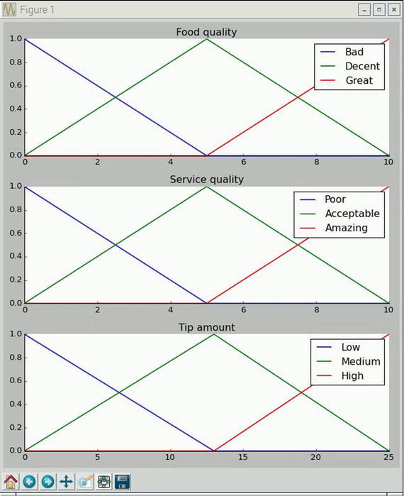
Figure 5-11. Three membership functions

Figure 5-12 shows the next display: the combined membership functions after all the rules are applied, and all the input and output membership are functions connected.

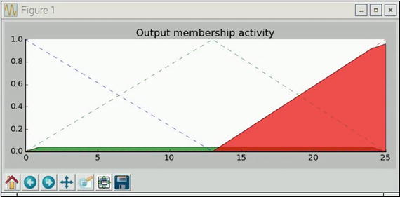
Figure 5-12. Membership functions after rules application

Figure 5-13 shows the next display: the post aggregation results for all the processed membership functions. In addition, there is a line indicating the crisp output for the tip percentage resulting from the defuzzification process.

Figure 5-13. Post aggregation and defuzzification results

Finally, Figure 5-14 shows the text display for the tip percentage, which comes from a print statement within the program.

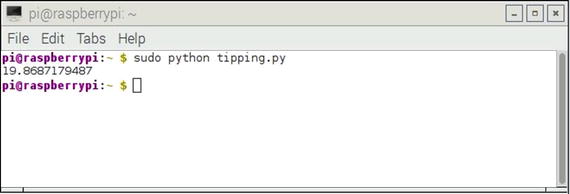
Figure 5-14. Print statement for tip percentage

Demo 5-2: Modifications to the tipping.py Program

In this section, I discuss modifications to the Python program to make it easier to use and significantly more portable. The main modification is to query the user about the food and service quality, rather than have static values, which was the case for the initial project. This modification is fairly easy and consists of creating two variables to hold the food and service quality levels, and two input statements to get the data into the program. The additional or modified code is as follows:

food_qual = raw_input('Rate the food quality, 0 to 10')
service_qual = raw_input('Rate the service quality, 0 to 10')

qual_level_lo = fuzz.interp_membership(x_qual, qual_lo, float(food_qual))
qual_level_md = fuzz.interp_membership(x_qual, qual_md, float(food_qual))
qual_level_hi = fuzz.interp_membership(x_qual, qual_hi, float(food_qual))

serv_level_lo = fuzz.interp_membership(x_serv, serv_lo, float(service_qual))
serv_level_md = fuzz.interp_membership(x_serv, serv_md, float(service_qual))
serv_level_hi = fuzz.interp_membership(x_serv, serv_hi, float(service_qual))

This modified code takes care of prompting the user to enter food and service quality ratings.

The second modification is to make the whole system completely portable, somewhat akin to the Nim game configuration discussed in the previous chapter. I would use an LCD display to show the user prompts to enter the food and the service quality ratings, and then show the resulting tip percentage. How cool would it be to have a portable fuzzy logic system that computes tip percentages to show off to your relatives and friends? The LCD display interface and software was discussed in the previous chapter. The only new required technology is a USB numeric key pad for the user to enter the quality ratings. Figure 5-15 shows a very inexpensive USB keypad that I experimented with for this modification. I am not going into all the details on how to complete this portable system, since I am reasonably confident that most of you can adapt the previous LCD discussions to this new application. Just remember, there is no longer a need for all the visualization code, which considerably reduces the size of the main program.

Figure 5-15. Inexpensive USB numeric keypad

This section completes the first project. It is now time to consider a more complex fuzzy logic controller project.

Demo 5-3: FLS Heating and Cooling System

I start this project assuming that you have read and understood the first project in the chapter. There should be no need to go into any detailed discussion regarding FL concepts. I simply follow the FLS algorithm in developing this project. In addition, I do not use any of the visualization code in this project because it already served its purpose in the previous project. Interested readers can easily reintroduce the code to obtain the plots to see how this system functions.

Consider a heating, ventilation, and cooling system (HVAC) that, practically speaking, is a heat pump that acts as either an air conditioner or a heater. Figure 5-16 shows a block diagram of such a system. This configuration is also known in control terminology as a closed-loop system.

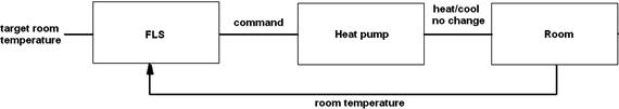
Figure 5-16. HVAC closed-loop system

Let’s define temperature (t) as a crisp input variable to represent the room temperature that is being heated or cooled. Generally, people use the terms hot and cold as room temperature qualifiers. These terms, as well as related ones, can be developed into a set of linguistic terms, such that

T(t) = { cold, comfortable,  hot }          

This expression for T(t) represents a decomposition function for the input variable t. Each member of this linguistic decomposition set represents or is associated with a numerical temperature range. For instance, cold could be a range of 40°F to 60°F, while hot might be a range of 70°F to 90°F. Other linguistic terms could easily fill in the intervening ranges if it was decided that 20°F was an appropriate interval value.

In addition, there is another input named target temperature, which is set by the people who occupy the room. This is analogous to setting a room thermostat.

Figure 5-17 shows the membership functions that were created to map the crisp, non-fuzzy, room and target temperature values to the corresponding fuzzy linguistic terms. Only one set of membership functions is shown because they are common to both the room and target temperature input variables.

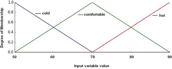
Figure 5-17. Room and target temperature membership functions

In this case, any given room temperature can belong to one or two groups, depending upon its values. Figure 5-18 shows that a room temperature of 65°F has a membership value of 0.5 in the comfortable membership function, as well as 0.5 in the cold membership function. A room temperature of exactly 70°F has a membership value of 1.0 and is only in the comfortable membership function.

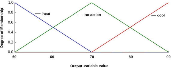
Figure 5-18. HVAC control membership functions

The HVAC controller also needs a set of membership functions to take based on command results. Figure 5-18 shows the set of membership functions for HVAC control. Note that it has the same shapes and output variable range as the input variables.

The following are some example rules to determine the control commands based on room and target temperatures:

• if (room temperature is cold ) and (target temperature is comfortable), then the command is heat

• if (room temperature is hot) and (target temperature is comfortable), then the command is cool

• if (room temperature is comfortable) and (target temperature is comfortable), then the command is no change

The precise command actions to be taken using a preset target temperature and measured room temperature have to be determined by a human expert and codified in the rules database. Table 5-3 is a matrix detailing the precise control commands for all combinations of linguistic variables for both room and target temperatures.

There are six rules required to accommodate all the combinations of the intersecting room temperature and target temperature linguistic terms that require action. The rules for no change are ignored. These are the rules :

• if room temp is cold and target temp is comfortable, then the command is heat

• if room temp is cold and target temp is hot, then the command is heat

• if room temp is comfortable and target temp is cold, then the command is cool

• if room temp is comfortable and target temp is heat, then the command is heat

• if room temp is hot and target temp is cold, then the command is cool

• if room temp is hot and target temp is comfortable, then the command is cool

Now that the set of rules have been created, it is time to discuss fuzzification.

import numpy as np
import skfuzzy as fuzz

# Generate universe variables
#   * room and target temperature range is 50 to 90
#   * same for the output control variable
x_room_temp    = np.arange(50, 91, 1)
x_target_temp  = np.arange(50, 91, 1)
x_control_temp = np.arange(50, 91, 1)

# Generate fuzzy membership functions
room_temp_lo     = fuzz.trimf(x_qual, [50, 50, 70])
room_temp_md     = fuzz.trimf(x_qual, [50, 70, 90])
room_temp_hi     = fuzz.trimf(x_qual, [70, 90, 90])
target_temp_lo   = fuzz.trimf(x_serv, [50, 50, 70])
target_temp_md   = fuzz.trimf(x_serv, [50, 70, 90])
target_temp_hi   = fuzz.trimf(x_serv, [50, 90, 90])
control_temp_lo  = fuzz.trimf(x_tip,  [50, 50, 70])
control_temp_md  = fuzz.trimf(x_tip,  [50, 70, 90])
control_temp_hi  = fuzz.trimf(x_tip,  [70, 90, 90])

# Get user inputs
room_temp = raw_input('Enter room temperature 50 to 90')
target_temp = raw_input('Enter target temperature 50 to 90')

# Calculate degrees of membership
room_temp_level_lo = fuzz.interp_membership(x_room_temp, room_temp_lo, float(room_temp))
room_temp_level_md = fuzz.interp_membership(x_room_temp, room_temp_md, float(room_temp))
room_temp_level_hi = fuzz.interp_membership(x_room_temp, room_temp_hi, float(room_temp))

target_temp_level_lo = fuzz.interp_membership(x_target_temp, target_temp_lo, float(target_temp))
target_temp_level_md = fuzz.interp_membership(x_target_temp, target_temp_md, float(target_temp))
target_temp_level_hi = fuzz.interp_membership(x_target_temp, Target_temp_hi, float(target_temp))

# Apply rule 1:  if room_temp is cold and target temp is comfortable then command is heat
# The 'and' operator means to take the minimum by using the 'np.fmin' function
active_rule1 = np.fmin(room_temp_level_lo, target_temp_level_md)
# Combine with hi control membership function using `np.fmin`
control_activation_1 = np.fmin(active_rule1, control_temp_hi)

# Next go through all five remaining rules
#Apply rule 2: if room_temp is cold and target temp is hot then command is heat
active_rule2 = np.fmin(room_temp_level_lo, target_temp_level_hi)
# Combine with hi control membership function using `np.fmin`
control_activation_2 = np.fmin(active_rule2, control_temp_hi)

#Apply rule 3: if room_temp is comfortable and target temp is cold then command is cool
active_rule3 = np.fmin(room_temp_level_md, target_temp_level_lo)
# Combine with lo control membership function using `np.fmin`
control_activation_3 = np.fmin(active_rule3, control_temp_lo)

#Apply rule 4: if room_temp is comfortable and target temp is heat then command is heat
active_rule4 = np.fmin(room_temp_level_md, target_temp_level_hi)
# Combine with hi control membership function using `np.fmin`
control_activation_4 = np.fmin(active_rule4, control_temp_hi)

#Apply rule 5: if room_temp is hot and target temp is cold then command is cool
active_rule5 = np.fmin(room_temp_level_hi, target_temp_level_lo)
# Combine with lo control membership function using `np.fmin`
control_activation_5 = np.fmin(active_rule5, control_temp_lo)

#Apply rule 6: if room_temp is hot and target temp is comfortable then command is cool
active_rule6 = np.fmin(room_temp_level_hi, target_temp_level_md)
# Combine with lo control membership function using `np.fmin`
control_activation_6 = np.fmin(active_rule6, control_temp_lo)

aggregated = np.fmax(control_activation_1, control_activation_2,
                     control_activation_3, control_activation_4,
                     control_activation_5, control_activation_6)

# Calculate defuzzified result using the method of centroids
control_value = fuzz.defuzz(x_control_temp, aggregated, 'centroid')

print control_value

import numpy as np
import skfuzzy as fuzz

# Generate universe variables
#   * room and target temperature range is 50 to 90
#   * same for the output control variable
x_room_temp    = np.arange(50, 91, 1)
x_target_temp  = np.arange(50, 91, 1)
x_control_temp = np.arange(50, 91, 1)

# Generate fuzzy membership functions
room_temp_lo     = fuzz.trimf(x_room_temp,   [50, 50, 70])
room_temp_md     = fuzz.trimf(x_room_temp,   [50, 70, 90])
room_temp_hi     = fuzz.trimf(x_room_temp,   [70, 90, 90])
target_temp_lo   = fuzz.trimf(x_target_temp, [50, 50, 70])
target_temp_md   = fuzz.trimf(x_target_temp, [50, 70, 90])
target_temp_hi   = fuzz.trimf(x_target_temp, [50, 90, 90])
control_temp_lo  = fuzz.trimf(x_control_temp,[50, 50, 70])
control_temp_md  = fuzz.trimf(x_control_temp,[50, 70, 90])
control_temp_hi  = fuzz.trimf(x_control_temp,[70, 90, 90])

# Get user inputs
room_temp = raw_input('Enter room temperature 50 to 90: ')
target_temp = raw_input('Enter target temperature 50 to 90: ')

# Calculate degrees of membership
room_temp_level_lo = fuzz.interp_membership(x_room_temp, room_temp_lo, float(room_temp))
room_temp_level_md = fuzz.interp_membership(x_room_temp, room_temp_md, float(room_temp))
room_temp_level_hi = fuzz.interp_membership(x_room_temp, room_temp_hi, float(room_temp))

target_temp_level_lo = fuzz.interp_membership(x_target_temp, target_temp_lo, float(target_temp))
target_temp_level_md = fuzz.interp_membership(x_target_temp, target_temp_md, float(target_temp))
target_temp_level_hi = fuzz.interp_membership(x_target_temp, target_temp_hi, float(target_temp))

# Apply all six rules
# rule 1:  if room_temp is cold and target temp is comfortable then command is heat
active_rule1 = np.fmin(room_temp_level_lo, target_temp_level_md)
control_activation_1 = np.fmin(active_rule1, control_temp_hi)

# rule 2: if room_temp is cold and target temp is hot then command is heat
active_rule2 = np.fmin(room_temp_level_lo, target_temp_level_hi)
control_activation_2 = np.fmin(active_rule2, control_temp_hi)

# rule 3: if room_temp is comfortable and target temp is cold then command is cool
active_rule3 = np.fmin(room_temp_level_md, target_temp_level_lo)
control_activation_3 = np.fmin(active_rule3, control_temp_lo)

# rule 4: if room_temp is comfortable and target temp is heat then command is heat
active_rule4 = np.fmin(room_temp_level_md, target_temp_level_hi)
control_activation_4 = np.fmin(active_rule4, control_temp_hi)

# rule 5: if room_temp is hot and target temp is cold then command is cool
active_rule5 = np.fmin(room_temp_level_hi, target_temp_level_lo)
control_activation_5 = np.fmin(active_rule5, control_temp_lo)

# rule 6: if room_temp is hot and target temp is comfortable then command is cool
active_rule6 = np.fmin(room_temp_level_hi, target_temp_level_md)
control_activation_6 = np.fmin(active_rule6, control_temp_lo)

# Aggregate all six output membership functions together
# Combine outputs to ease the complexity as fmax() only as two args
c1 = np.fmax(control_activation1, control_activation2)
c2 = np.fmax(control_activation3, control_activation4)
c3 = np.fmax(control_activation5, control_activation6)
c4 = np.fmax(c2,c3)
aggregated = np.fmax(c1, c4)

# Calculate defuzzified result using the method of centroids
control_value = fuzz.defuzz(x_control_temp, aggregated, 'centroid')

#  Display the crisp output value
print control_value

Demo 5-4: Modifications to the HVAC Program

For this demo, I made a simple modification to the control program: one of three LEDs lights up, based on whether heating, cooling, or no change is determined from user input. The following code is appended to the prior listing, except the additional import and configuration statements should be placed at the start of the program, just as I did with previous programs that used LEDs. I provide comments that indicate the GPIO pins used in this modification. They are the same ones that were used in the prs.py game, so use the LED interconnection diagram shown in that project.

# Include the following at the beginning of the hvac.py program
import RPi.GPIO as GPIO
import time

# Setup GPIO pins
# Set the BCM mode
GPIO.setmode(GPIO.BCM)

# Outputs
GPIO.setup( 4, GPIO.OUT) # heat command
GPIO.setup(17, GPIO.OUT) # cool command
GPIO.setup(27, GPIO.OUT) # no change command

# Ensure all LEDs are off to start
GPIO.output( 4, GPIO.LOW)
GPIO.output(17, GPIO.LOW)
GPIO.output(27, GPIO.LOW)

# The following should be appended to the existing code
if control_value > 65 and control_value < 75: # no change
    GPIO.output(27, GPIO.HIGH)
    time.sleep(5)
    GPIO.output(27, GPIO.LOW)
elif control_value > 82 and control_value < 84: # heat
    GPIO.output(4, GPIO.HIGH)
    time.sleep(5)
    GPIO.output(4, GPIO.LOW)
elif control_value > 56 and control_value < 68: # cool
    GPIO.output(17, GPIO.HIGH)
    time.sleep(5)
    GPIO.output(17, GPIO.LOW)
else:
    print 'strange value calculated'
# This next statement used in debugging phase
print 'Thats all folks'

hvac_led.py—the complete program with the LED modifications—is available on this book’s website. Figure 5-19 shows the Raspberry Pi physical setup with the three control LEDs connected to a solderless breadboard.

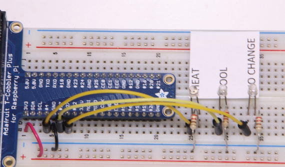
Figure 5-19. Physical setup

Summary

This chapter focused on fuzzy logic, which is a very clever approach to handling non-precise values that are present in almost every human situation. My approach was to use several practical projects to bring fuzzy logic into an understandable framework from where you could develop your own FL projects.

This chapter had very detailed demonstrations, including a seven-step algorithm for developing a fuzzy logic system (FLS).

The first demonstration showed how to compute a tip based on food quality and service quality. The seven-step algorithm resulted in a program that quickly computed a tip percentage based on user ratings. I even suggested a way to make the project completely portable.

The second demonstration was somewhat more technical than the first. It involved creating a heating and cooling FL control system. This system type is commercially available in HVAC products. In fact, one manufacturer advertises that its system incorporates fuzzy logic. Admittedly, this chapter’s project is a scaled-down version of a commercial HVAC system, but it nonetheless incorporates all the important parts of an FLS.