Parts List

For the second demonstration, you need the parts that are listed in Table 11-1.

There is a robot used in a demonstration discussed in this chapter that you can build by following the instructions in the appendix. The parts list includes items required beyond those needed for the basic robot.

The underlying formal structure for BBR is called subsumption architecture . In 1985, MIT professor Dr. Rodney Brooks wrote an internal technical memo titled “A Robust Layered Control Mechanism for Mobile Robots.” At the time, Dr. Brooks worked in MIT’s Artificial Intelligence Laboratory. His memo was subsequently published in 1986 as a paper in the IEEE Journal of Robotics and Automation. His paper changed the nature and direction of robotics research for many years. The gist of the paper described a robot control organization that he called subsumption architecture. The theory behind this architecture is based, in part, on the evolutionary development of the human brain.

Human Brain Structure

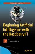
On a very broad scale, the human brain can be divided into three levels or parts. The lowest level is the most primitive part, which is responsible for basic life-supporting activities, such as respiration, blood pressure, core temperature, and so forth. The brain stem is the organic brain section that hosts these primitive functions. Figure 11-1 illustrates the brain stem and the limbic system.

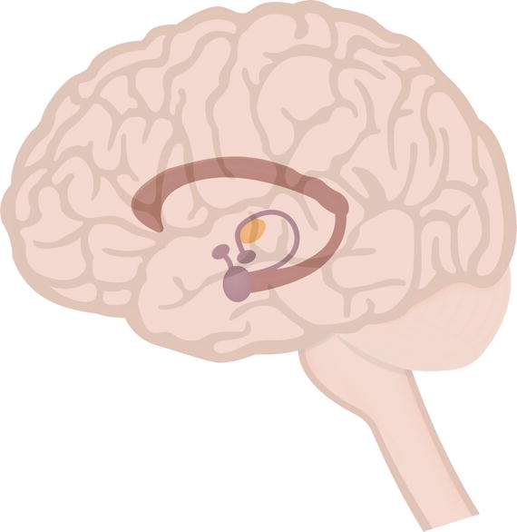
Figure 11-1. Brain stem and limbic system

The next highest level of brain function has been termed the reptile brain or limbic system. It is responsible for eating, sleeping, reproduction, flight or fight, and similar behaviors. The limbic system is made up of the hippocampus, amygdala, hypothalamus, and the pituitary gland. Finally, the highest cognitive level is the neocortex, which is responsible for learning, thinking, and similar high-level complex activities. The brain components composing the neocortex, or cerebral cortex, are the frontal, temporal, occipital, and parietal lobes. Figure 11-2 illustrates the four lobes that comprise the cerebral cortex.

Figure 11-2. Cerebral cortex

Most often, these various brain levels function quite independently of each other but they can and often have conflicts. Perhaps you have a “high-strung” personality and find food a welcoming diversion to ease stress. The higher-level function knows that eating too much of the wrong types of food is no good for you, but the lower-level reptile brain still craves it. Which brain level overrides and changes your behavior is problematic. Sometimes the lower level wins and other times the higher level wins. However, if you have an addiction, it is always the case that the lower level wins and changes your behavior, usually for the worst. Anyone can have many different brain-level behaviors ready to activate at a given time, but only one “wins” out and causes the current active behavior to be displayed. This interplay between brain behaviors was one source of Dr. Brooks’ subsumption architecture.

Subsumption Architecture

A definition of subsumption will help at this point in the discussion. However, what really has to be defined is the word subsume, because subsumption is circularly defined as the act of subsuming.

subsume: incorporating something under a more general category; to include something in a larger group or a group in a higher position

These definitions imply that complex behaviors can be decomposed into multiple simpler behaviors. There is another perspective that must be added to the definition. This addition is the word reactive, because in the real world, robots depend on sensors to react or change behaviors based on sensory inputs. These inputs are constantly reacting to changes in the robot’s environment. Reactive behavior is also called stimulus/response behavior, which is appropriate for insects. Insects are a lower-level life form when compared to mammals, and they do not have a highly developed learning capability. What they do have is called habituation, which allows an insect to adapt to certain types of environmental changes. This can easily be seen by blowing air on a cockroach. The insect initially retreats from the blowing air. However, repeatedly blowing air on the cockroach causes it to ignore the air because it is perceived as non–life threatening. This type of low-level learning is useful for robots, especially autonomous robots.

One way to display the traditional approach for a reactive system is shown in Figure 11-3.

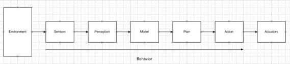
Figure 11-3. Flowchart for a sensor-based system

The collection of serial processes, from sensors to action, may be thought of as a behavior. This layout of serial processes or tasks is slow and relatively inflexible. Sensors acquire data without attempting to process it in any way. That job is left to the perception block, which must sort out all relevant sensory data before passing it on to the model block. The model block transforms this filtered data into a contextual sense or state. The plan block has rules that are followed based upon the state it receives from the model block. Finally, the action block implements the appropriate rules received from the plan block and sends the required control signals to the actuators, which are shown in the final block in the diagram. Having all of these blocks in a serial architecture makes for a slow response, which is not a good robotic attribute.

The serial blocks shown in the diagram represent a complex behavior that can be represented by a single layer. A layer in a behavioral sense may be considered a goal to be achieved by an agent or a robot.

Complex behaviors maybe decomposed into simpler behaviors. This is the key to subsumption architecture. Figure 11-4 shows a two-layer decomposition in place of the complex single-layer behavior stream shown in Figure 11-3.

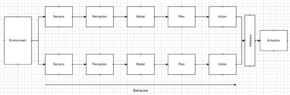
Figure 11-4. Two-layer behavior serial stream

Each layer or path is considered related to a specific task, such as following a wall or detecting an obstacle. This is the subsumption architecture proposed by Dr. Brooks. Notice that there is an additional arbitrator block that processes all of the action block signals before sending selected ones to the actuators. This arbitrator block is another important element in subsumption architecture.

Systems can be made much more responsive by essentially converting a single, complex behavior into multiple parallel paths. It is also easy to envision that many more layers can be added without disturbing any of the existing layers. The feature of extending code without modifying existing code closely mimics the software composition principle discussed in an earlier chapter. It is always a good thing to be able to extend existing code without too much “disturbance” to the existing code.

The subsumption architecture does not provide any guidance on how to decompose a complex behavior into simpler multiple tasks. In addition, the perception block is generally regarded as the hardest of all the blocks to define and implement. The problem is to create a meaningful data set from a limited number of environmental sensors. This data set then feeds the model block that effectively creates the robot’s world or state. At this point, BBR differs significantly from the more traditional approach. I discuss the traditional approach first, followed by the BBR approach.

Behavior-Based Robotics Approach

It is worth digressing a bit before discussing BBR. In the study of animal behavior, also known as ethology, it has been shown that infant seagulls respond to parent models. Figure 11-5 shows such a parent model with a feature circled in the figure, which will trigger the infant gull’s instinct feeding behavior.

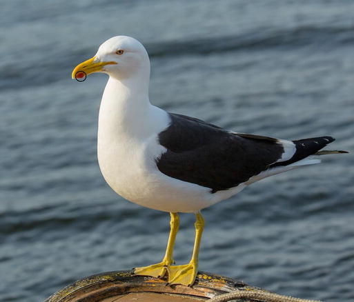
Figure 11-5. Seagull ethology

All that matters to the infant gulls is that the parent gull model has a sharp beak with a colored spot near the beak tip. The babies open their beaks awaiting food delivery. These infant gulls use a very limited real-world representation, but it has been shown to be perfectly adequate for the gull species to survive.

Similarly, real-world robots can use a limited real-world representation or model, so that it should be adequate to carry out the desired requirements without reliance on an overly detailed world model.

These limited representations are often referred to as “snapshots” of the local environment. Behaviors are then designed to react to these snapshots. Two of the important points are that the mobile robot does not need to maintain a geometric coordinate system, and it does not have to have a memory-laden real-world model. By utilizing reflex-like direct responses, mobile robots minimize the complexity of the model, plan, and action blocks. The behavior stream almost reverts to a simple behavior diagram, as shown in Figure 11-6.

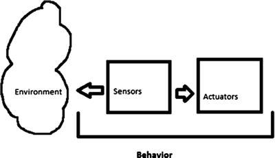
Figure 11-6. Simple behavioral stream

How can environmental snapshots be related to robot behaviors? Initially, a data set has to be created that consists of the sensor data generated when the environmental conditions exist, which should trigger the desired robotic reflexive behavior. These are termed sensor signatures. Now all that needs to be done is to link the signatures to a specific behavior using interpretive routines, normally done in the Prediction block. However, there could be an issue that given the relatively coarse-grained sensor data signatures, simultaneous stimulus/response pairings could happen. Assigning priorities to the simple behaviors alleviates this situation. In addition, default or long-term behaviors are normally assigned a lower priority than emergent or “tactical” behaviors. The tactical signature happens if the robot encounters an environment condition that requires immediate attention from the robot control system.

Instituting a behavior prioritization scheme has an unintended positive outcome. Robots usually operate with the same behavior, such as moving forward. All behaviors acting in sequence should strive to maintain this normalcy. Only when environmental conditions warrant should a behavior direct the robot to deviate from the normal. When deviations happen, the higher-priority behaviors take control and try to restore normalcy.

BBR also incorporates long-term progress indicators to help avoid a “looping” situation, as might be the case where the robot continually bounces between two barriers or is locked into a wall corner. These long-term progress indicators effectively generate a strategic trajectory in which the robot moves in a general direction or path. When progress is impeded, a different set of behaviors is selected to return to the normal state.

In a layered subsumption model, a low-level layer might have the goal to “avoid an obstacle.” This layer could be “beneath” a higher level of “roam around.” The higher level of “roam around” is said to subsume the lower-level behavior of “avoid an obstacle.” All layers have access to sensors to detect environment changes, as well as the ability to control actuators. An overall constraint is that separate tasks have the ability to suppress any input and to inhibit output sent to actuators. In this way, the lowest levels can be very responsive to environment changes, much the way reflexes function in living organisms. Higher levels are more abstract and devoted to satisfying goals.

The following behaviors may be represented by a variety of graphical or mathematical models :

• Functional notation

• Stimulus/response diagram

• Finite state machine (FSM)

• Schema

I use the FSM model because it provides a good representation of behavior interactions without much mathematic abstraction. A basic FSM model is shown in Figure 11-7.

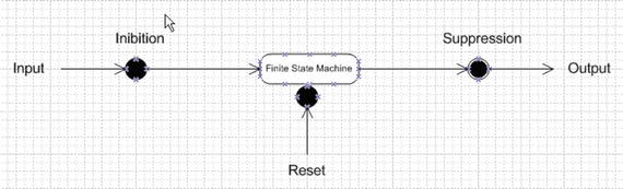
Figure 11-7. Basic FSM model

Figure 11-8 shows multiple behaviors with interrelationships, including sensory inhibitions and actuator suppressions. Notice the layered behavior sequences and behavior prioritization discussed earlier.

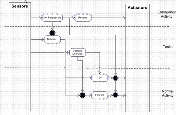
Figure 11-8. Multilayered FSM model

At this point in the discussion, I would normally proceed to show you a Python implementation for a subsumption architecture that runs on a Raspberry Pi. Next, however, I divert from the norm to discuss a very nice robot simulation project that can implement subsumption and a whole lot more.

Demo 11-1: The Breve Project

The breve project is the work of Jon Klein, who developed it as part of his undergraduate and graduate thesis work. It is available from Jon’s website at www.spiderland.org for Windows, Linux, and Mac platforms. I am using it on a MacBook Pro and it seems to perform quite flawlessly. Just be aware that Jon states on his website that he is no longer actively updating the application but continues to make it available, at least in the Mac format.

Here are Jon’s own words to describe what breve is all about: “breve is a free, open-source software package which makes it easy to build 3D simulations of multi-agent systems and artificial life. Using Python, or using a simple scripting language called steve, you can define the behaviors of agents in a 3D world and observe how they interact. breve includes physical simulation and collision detection so you can simulate realistic creatures. It also has an OpenGL display engine so you can visualize your simulated worlds.”

There is extensive HTML-formatted documentation on the website that I urge you to review; particularly the introductory pages showing how to run one of the many available demo scripts. These scripts are both in the “steve” front-end language as well as Python. It is impossible for me to go through the many documentation pages, which would constitute an entire book to itself. I did run the following Python script, titled RangerImage.py , in breve. The listing is shown here to provide a glimpse of the power and flexibility that you have using breve.

import breve

class AggressorController( breve.BraitenbergControl ):
    def __init__( self ):
        breve.BraitenbergControl.__init__( self )
        self.depth = None
        self.frameCount = 0
        self.leftSensor = None
        self.leftWheel = None
        self.n = 0
        self.rightSensor = None
        self.rightWheel = None
        self.simSpeed = 0
        self.startTime = 0
        self.vehicle = None
        self.video = None
        AggressorController.init( self )

    def init( self ):
        self.n = 0
        while ( self.n < 10 ):
            breve.createInstances( breve.BraitenbergLight, 1 ).move( breve.vector( ( 20 * breve.breveInternalFunctionFinder.sin( self, ( ( self.n * 6.280000 ) / 10 ) ) ), 1, ( 20 * breve.breveInternalFunctionFinder.cos( self, ( ( self.n * 6.280000 ) / 10 ) ) ) ) )
            self.n = ( self.n + 1 )

        self.vehicle = breve.createInstances( breve.BraitenbergVehicle, 1 )
        self.watch( self.vehicle )
        self.vehicle.move( breve.vector( 0, 2, 18 ) )
        self.leftWheel = self.vehicle.addWheel( breve.vector( -0.500000, 0, -1.500000 ) )
        self.rightWheel = self.vehicle.addWheel( breve.vector( -0.500000, 0, 1.500000 ) )
        self.leftWheel.setNaturalVelocity( 0.000000 )
        self.rightWheel.setNaturalVelocity( 0.000000 )
        self.rightSensor = self.vehicle.addSensor( breve.vector( 2.000000, 0.400000, 1.500000 ) )
        self.leftSensor = self.vehicle.addSensor( breve.vector( 2.000000, 0.400000, -1.500000 ) )
        self.leftSensor.link( self.rightWheel )
        self.rightSensor.link( self.leftWheel )
        self.leftSensor.setBias( 15.000000 )
        self.rightSensor.setBias( 15.000000 )
        self.video = breve.createInstances( breve.Image, 1 )
        self.video.setSize( 176, 144 )
        self.depth = breve.createInstances( breve.Image, 1 )
        self.depth.setSize( 176, 144 )
        self.startTime = self.getRealTime()

    def postIterate( self ):
        self.frameCount = ( self.frameCount + 1 )
        self.simSpeed = (self.getTime()/(self.getRealTime()- self.startTime))
        print '''Simulation speed = %s''' % (  self.simSpeed )
        self.video.readPixels( 0, 0 )
        self.depth.readDepth( 0, 0, 1, 50 )
        if ( self.frameCount < 10 ):
            self.video.write( '''imgs/video-%s.png''' % (self.frameCount))

        self.depth.write16BitGrayscale('''imgs/depth-%s.png''' % (self.frameCount))

breve.AggressorController = AggressorController

# Create an instance of our controller object to initialize the simulation
AggressorController()

Figure 11-9 shows the actual robot running in the breve display, which was created by the preceding script.

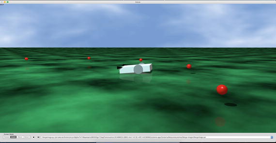
Figure 11-9. breve world

You may have noticed in the script that there are references to BraitenbergControl, BraitenbergLight, and BraitenbergVehicle. These are based on a thought experiment conducted by Italian-Austrian cyberneticist Valentino Braitenberg, who wrote Vehicles: Experiments in Synthetic Psychology (The MIT Press,1984), which I highly recommend for readers desiring to learn more about his innovative approach to robotics. In his experiment, he envisions vehicles directly controlled by sensors. The resulting behavior might appear complex, or even intelligent, but in reality, it is based on a combination of simpler behaviors. That should remind you of subsumption at work.

A Braitenberg vehicle may be thought of as an agent that autonomously moves around based on its own sensory inputs. In these thought experiments, the sensors are primitive and simply measure a stimulus, which is often just a point light source. The sensors are also directly connected to the motor actuators so that a sensor can immediately activate a motor upon stimulation. Again, this should remind you of the simple behavioral stream shown in Figure 11-4.

The resulting Braitenberg vehicle behavior depends on how the sensors and motors are connected. In Figure 11-10, there are two different configurations between the sensors and the motors. The vehicle to the left is wired so that it avoids or drives away from the light source. This contrasts with the vehicle on the right, which drives toward the light source.

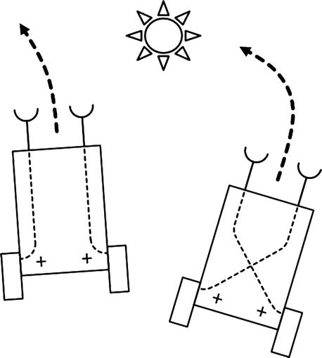
Figure 11-10. Braitenberg vehicles

It is not too much of a leap to say that the vehicle on the left “fears” the light, while the vehicle on the right “likes” the light. I have assigned human-like behaviors to a robot, which is precisely the result that Braitenberg was seeking.

Another Braitenberg vehicle has one light sensor with the following behaviors :

• More light produces faster movement.

• Less light produces slower movement.

• Darkness produces standstill.

This behavior can be interpreted as a robot that is afraid of the light and moves quickly to get away from it. Its goal is to find a dark spot to hide.

Of course, the complementary Braitenberg vehicle is one that features these behaviors:

• More darkness produces faster movement.

• Less darkness produces slower movement.

• Full light produces standstill.

In this case, the behavior can be interpreted as a robot that is seeking light and moves quickly to get to it. Its goal is to find the brightest spot to park.

Braitenberg vehicles exhibit complex and dynamic behavior in a complex environment with multiple stimulation sources. Depending on the configuration between the sensors and the actuators, a Braitenberg vehicle might move close to a source, but not touch it, run away very quickly, or make circles or figures-of-eight around a point. Figure 11-11 illustrates these complex behaviors.

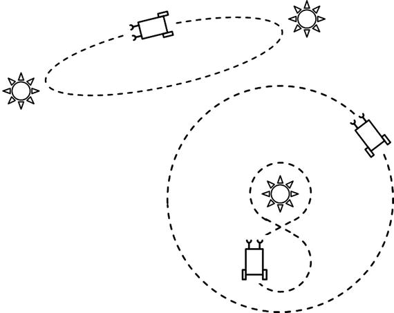
Figure 11-11. Braitenberg vehicles with complex behaviors

These behaviors may appear to be goal-directed, adaptive, and even intelligent in much the same way that minimal intelligence is attributed to a cockroach’s behavior. But the truth is that the agent is functioning in a purely mechanical way, without any cognitive or reasoning processes at play.

There are a few items in the breve Python example that I want to further explain in preparation for a step-by-step example in which you create your own Braitenberg vehicle. The first item to note is that all breve simulations require a controller object, which specifies how the simulation is to be set up. The controller’s name in this simulation is AggressorController. In the controller definition, there is at least one initialization method named init. In this specific case, because this is a Python script, there is another initialization method named __init__. The first initialization method is called when a breve object is instantiated. The second initialization method is automatically called when a Python object is instantiated. breve takes care of sorting out the relationships between breve and Python objects using a third object called a bridge. You don’t ordinarily have to be concerned with these bridge objects. In fact, if you only use the steve scripting language (instead of Python), you never see a bridge object.

The init method creates 10 Braitenberg light objects, a few of which you can see in Figure 11-7. They are the spheres named 'n' surrounding the Braitenberg robot, which is also created by the init method and is referred to as vehicle.

The __init__ method creates all the attributes needed for the simulation, and then it calls the init method that instantiates all the required simulation objects and assigns real values to the attributes. Once that is accomplished, all that is needed to click the play button to view the simulation.

The step-by-step demonstration starts here. The following listing creates a non-functioning Braitenberg vehicle and a light source:

import breve
class Controller(breve.BraitenbergControl):
    def __init__(self):
        breve.BraitenbergControl.__init__(self)
        self.vehicle = None
        self.leftSensor = None
        self.rightSensor = None
        self.leftWheel = None
        self.rightWheel = None
        self.simSpeed = 0
        self.light = None
        Controller.init(self)

    def init(self):
        self.light = breve.createInstances(breve.BraitenbergLight, 1)
        self.light.move(breve.vector(10, 1, 0))
        self.vehicle = breve.createInstances(breve.BraitenbergVehicle, 1)
        self.watch(self.vehicle)

    def iterate(self):
        breve.BraitenbergControl.iterate(self)

breve.Controller = Controller
Controller()

I named this script firstVehicle.py to indicate that it is the first of several generated in the process of developing a working simulation. Figure 11-12 shows the result after I loaded and “played” this script in the breve application.

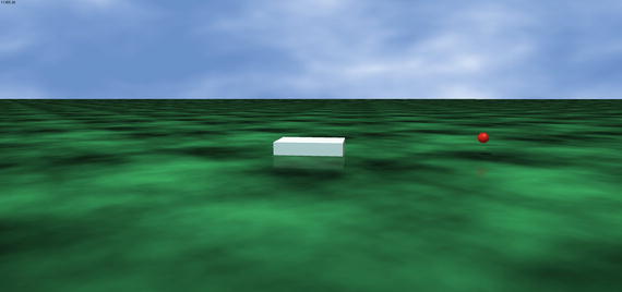
Figure 11-12. breve world for the firstVehicle script

This script defines a Controller class that has the two initialization methods mentioned earlier. The init method instantiates a Braitenberg light object and a Braitenberg vehicle. The __init__ method creates a list of attributes, which is filled in by a follow-on script. This method also calls the init method.

There is also a new method called iterate that simply causes the simulation to run continuously.

The next step in developing the script is to add sensors and wheels to the vehicle to allow it to move through and explore the breve world. The following statements add the wheels and set an initial velocity that causes the vehicle to turn in circles. These statements go into the init method .

self.vehicle.move(breve.vector(0, 2, 18))
self.leftWheel = self.vehicle.addWheel(breve.vector(-0.500000,0,-1.500000))
self.rightWheel = self.vehicle.addWheel( breve.vector(-0.500000,0,1.500000))
self.leftWheel.setNaturalVelocity(0.500000)
self.rightWheel.setNaturalVelocity(1.000000)

The next set of statements adds the sensors. These are also added to the init method. The sensors are also cross-linked between the wheels (i.e., right sensor controls the left wheel and vice versa). The setBias method sets the amount of influence that a sensor has on its linked wheel. The default value is 1, which means that the sensor has a slightly positive influence on the wheel. A value of 15 means that the sensor has a strongly positive influence on the wheel. Bias can also be negative, meaning the influence is directly opposite to wheel activation.

self.rightSensor = self.vehicle.addSensor(breve.vector(2.000000, 0.400000, 1.500000))
self.leftSensor = self.vehicle.addSensor( breve.vector(2.000000, 0.400000, -1.500000 ) )
self.leftSensor.link(self.rightWheel)
self.rightSensor.link(self.leftWheel)
self.leftSensor.setBias(15.000000)
self.rightSensor.setBias(15.000000)

The preceding sets of statements were added to the init method. The whole script name was changed to secondVehicle.py. The sensors are designed to have a natural affinity toward any light source. However, if the sensors do not detect any light source, they will not activate their respective linked wheels. In this script configuration, the sensors do not immediately detect the light source and the vehicle simply stays still, which is the reason for my setting an initial natural velocity for each wheel. These settings guarantee that the robot will move. It may not move in the direction of the light source, but it moves. Figure 11-13 shows the updated breve world with the enhanced vehicle.

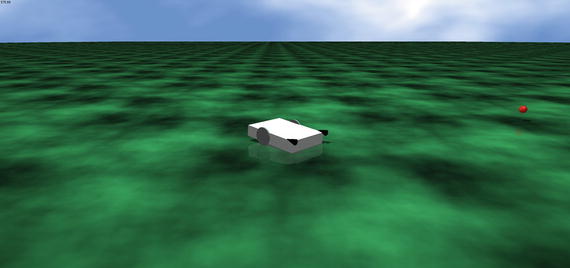
Figure 11-13. Breve world for the secondVehicle script

At this stage, the simulation is working, but it is a bit dull because the vehicle has no purpose other than to turn in circles in the breve world, and perhaps to catch a glimpse of the solitary light source. It is time to give the vehicle a better goal to realize the rationale behind a simulation. I make the goal really simple, as this is a “hello world” type demonstration and its purpose is to clarify, not obscure how a breve simulation works. The goal is to have the vehicle seek out a number of light sources and simply “run through” them.

These additional Braitenberg light sources are generated by the following loop that is added to the init method.

self.n = 0
    while (self.n < 10):
        breve.createInstances( breve.BraitenbergLight, 1).move( breve.vector((20 * breve.breveInternalFunctionFinder.sin(self, ((self.n * 6.280000) / 10))), 1,(20 * breve.breveInternalFunctionFinder. cos(self, ((self.n * 6.280000 ) / 10)))))
        self.n = ( self.n + 1 )

I also commented out the single light source created in the initial script. In addition, I reset the natural velocities back to 0.0 because there are now a sufficient number of light sources that the vehicle sensors can likely detect. Figure 11-14 shows the updated breve world, with some of the additional light sources and the vehicle going through them. The new script was renamed thirdVehicle.py.

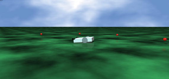
Figure 11-14. breve world for the thirdVehicle script

This last script completes my introductory lesson on how to create a robot simulation in the breve environment using Python. This lesson just scratches the surface on what breve has to offer—not just in robotic simulations but in a whole host of other AI applications. Look at Figure 11-15 and see if you recognize it.

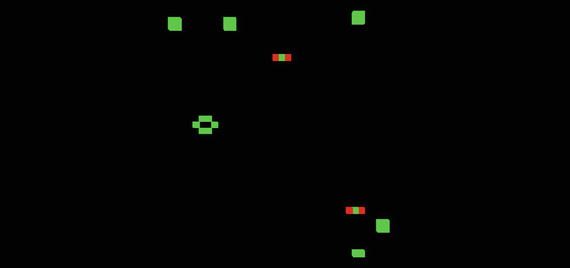
Figure 11-15. breve snapshot

It is a snapshot of Conway’s Game of Life running in breve. This script is named PatchLife.py. It is available in the Demos menu selection in both Python and steve formats . In fact, most demos are available in both formats. There are many demos available for you to try, including the following:

• Braitenberg: vehicles, lights

• Chemistry: Gray Scott diffusion, hypercycle

• DLA: diffusion limited aggression (fractal growth)

• Genetics: Game of Life both 2D and 3D

• Music: play midi and wav files

• Neural networks: multilayer

• Physics: springs, joints, walkers

• Swarms: swarming robots and other lifeforms

• Terrain: robots, creatures exploring terrain features

It is now time to conclude the breve discussion and return to subsumption.

Demo 11-2: Building a Subsumption-Controlled Robot Car

This section’s objective is to describe how to program a Raspberry Pi that directly controls a robot car. The robot car is the same platform used in Chapter 7, but now uses subsumption architecture to control the car’s behaviors. Python is the implementation language for the subsumption classes and scripts.

After searching through GitHub, I was inspired by Alexander Svenden’s EV3 post that used Python to implement a generic subsumption structure. I also relied on my experience with developing subsumptive Java classes with leJOS. You can read more about these Java classes at www.lejos.org . There are two primary classes required: one abstract class named Behavior and the other named Controller. The Behavior class encapsulates the car’s behavior using the following methods :

• takeControl() : Returns a Boolean value indicating if the behavior should take control or not.

• action() : Implements the specific behavior done by the car.

• suppress() : Causes the action behavior to immediately stop, and then returns the car state to one in which the next behavior can take control.

import RPi.GPIO as GPIO
import time
class Behavior(self):
    global pwmL, pwmR

    # use the BCM pin numbers
    GPIO.setmode(GPIO.BCM)

    # setup the motor control pins
    GPIO.setup(18, GPIO.OUT)
    GPIO.setup(19, GPIO.OUT)

    pwmL = GPIO.PWM(18,20) # pin 18 is left wheel pwm
    pwmR = GPIO.PWM(19,20) # pin 19 is right wheel pwm

    # must 'start' the motors with 0 rotation speeds
    pwmL.start(2.8)
    pwmR.start(2.8)

The Controller class contains the main subsumption logic that determines which behaviors are active based on priority and the need for activation. The following are some of the methods in this class:

• __init__(): Initializes the Controller object.

• add(): Adds a behavior to the list of available behaviors. The order in which they are added determines the behavior’s priority.

• remove(): Removes a behavior from the list of available behaviors. Stops any running behavior if the next highest behavior overrides it.

• update(): Stops an old behavior and runs the new behavior.

• step(): Finds the next active behavior and runs it.

• find_next_active_behavior(): Finds the next behavior wishing to be active.

• find_and_set_new_active_behavior(): Finds the next behavior wishing to be active and makes it active.

• start(): Runs the selected action method.

• stop(): Stops the current action.

• continously_find_new_active_behavior(): Monitors in real-time for new behaviors desiring to be active.

• __str__(): Returns the name of the current behavior.

The Controller object also functions as a scheduler, where one behavior is active at a time. The active behavior is decided by the sensor data and its priority. Any old active behavior is suppressed when a behavior with a higher priority signals that it wants to run.

There are two ways to use the Controller class . The first way is to let the class take care of the scheduler itself by calling the start() method. The other way is to forcibly start the scheduler by calling the step() method.

import threading
class Controller():

    def __init__(self):
        self.behaviors = []
        self.wait_object = threading.Event()
        self.active_behavior_index = None

        self.running = True
        #self.return_when_no_action = return_when_no_action

        #self.callback = lambda x: 0

    def add(self, behavior):
        self.behaviors.append(behavior)

    def remove(self, index):
        old_behavior = self.behaviors[index]
        del self.behaviors[index]
        if self.active_behavior_index == index:  # stop the old one if the new one overrides it
            old_behavior.suppress()
            self.active_behavior_index = None

    def update(self, behavior, index):
        old_behavior = self.behaviors[index]
        self.behaviors[index] = behavior
        if self.active_behavior_index == index:  # stop the old one if the new one overrides it
            old_behavior.suppress()

    def step(self):
        behavior = self.find_next_active_behavior()
        if behavior is not None:
            self.behaviors[behavior].action()
            return True
        return False

    def find_next_active_behavior(self):
        for priority, behavior in enumerate(self.behaviors):
            active = behavior.takeControl()
            if active == True:
                activeIndex = priority
        return activeIndex

    def find_and_set_new_active_behavior(self):
        new_behavior_priority = self.find_next_active_behavior()
        if self.active_behavior_index is None or self.active_behavior_index > new_behavior_priority:
            if self.active_behavior_index is not None:
                self.behaviors[self.active_behavior_index].suppress()
            self.active_behavior_index = new_behavior_priority

    def start(self):  # run the action methods
        self.running = True
        self.find_and_set_new_active_behavior()  # force it once
        thread = threading.Thread(name="Continuous behavior checker",
                                target=self.continuously_find_new_active_behavior, args=())
        thread.daemon = True
        thread.start()

        while self.running:
            if self.active_behavior_index is not None:
                running_behavior = self.active_behavior_index
                self.behaviors[running_behavior].action()

                if running_behavior == self.active_behavior_index:
                    self.active_behavior_index = None
                    self.find_and_set_new_active_behavior()
            self.running = False

    def stop(self):
        self._running = False
        self.behaviors[self.active_behavior_index].suppress()

    def continuously_find_new_active_behavior(self):
        while self.running:
            self.find_and_set_new_active_behavior()

    def __str__(self):
        return str(self.behaviors)

The Controller class is very general by allowing a wide variety of behaviors to be implemented using the general-purpose methods. The takeControl() method allows a behavior to signal that it wishes to take control of the robot. The way it does this is discussed later. The action() method is the way a behavior starts to control the robot. The obstacle avoidance behavior kicks off its action() method if a sensor detects an obstacle impeding the robot’s path. The suppress() method is used by a higher priority behavior to stop or suppress the action() method of a lower priority behavior. This happens when an obstacle avoidance behavior takes over from the normal forward motion behavior by suppressing the forward behavior’s action() method and having its own action() method activated.

The Controller class requires a list or array of Behavior objects that comprise the robot’s overall behavior. A Controller instance starts with the highest array index in the Behavior array and checks the takeControl() method’s return value. If true, it calls that behavior’s action() method. If it is false, the Controller checks the next Behavior object’s takeControl() method return value. Prioritization happens by the assignment of index array values attached to each Behavior object. The Controller class continually rescans all the Behavior objects and suppresses a lower priority behavior if a higher priority behavior asserts the takeControl() method while the lower priority action() method is activated. Figure 11-16 shows this process with all the behaviors that are eventually added.

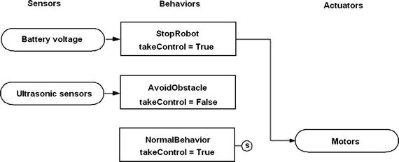
Figure 11-16. Behavior state diagram

It is now time to create a relatively simple behavior-based robot example.

Demo 11-3: Alfie Robot Car

The target robot is Alfie, which was used in previous chapters. The normal or low-priority behavior is to drive in a forward direction. A higher-priority behavior is obstacle avoidance, which uses ultrasonic sensors to detect obstacles in the robot’s direct path. The obstacle avoidance behavior is to stop, back up, and turn 90 degrees to the right.

The following class is named NormalBehavior. It reinforces the layered behavior approach. This class has all the required Behavior method implementations.

class NormalBehavior(Behavior):
    def takeControl():
        return true
    def action():
        # drive forward
        pwmL.ChangeDutyCycle(3.6)
        pwmR.ChangeDutyCycle(2.2)
    def suppress():
        # all stop
        pwmL.ChangeDutyCycle(2.6)
        pwmR.ChangeDutyCycle(2.6)

The takeControl() method should always return the logical value true. Higher priority behaviors are always allowed control by the Controller class; it really doesn’t matter if this lower priority requests control.

The action() method is very simple: power the motors in a forward direction using the full-power setting.

The suppress() method is also very simple: it stops both motors.

The obstacle avoidance behavior is a bit more complex, however. It still implements the same three methods specified in the Behavior interface. I named the class AvoidObstacle to indicate its basic behavior.

class AvoidObstacle(Behavior):
global distance1, distance2
    def takeControl():
        if distance1 <= 25.4 or distance2 <= 25.4:
            return True
        else:
            return False

    def action():
        # drive backward
        pwmL.ChangeDutyCycle(2.2)
        pwmR.ChangeDutyCycle(3.6)
        time.sleep(1.5)
        # turn right
        pwmL.ChangeDutyCycle(3.6)
        pwmR.ChangeDutyCycle(2.6)
        time.sleep(0.3)
        # stop
        pwmL.ChangeDutyCycle(2.6)
        pwmR.ChangeDutyCycle(2.6)

    def suppress():
        # all stop
        pwmL.ChangeDutyCycle(2.6)
        pwmR.ChangeDutyCycle(2.6)

There are a few items to point out regarding this class. The takeControl() method returns a logical true only if the distance between the ultrasonic sensor and the obstacle is 10 inches or less. This behavior is never active without asserting a true value.

The action() method causes the robot to back up for 1.5 seconds, as seen by the time.sleep(1.5) statement. The robot next rotates for 0.3 seconds based on stopping the right motor and allowing the left motor to continue to run. The robot then stops waiting for the next behavior to activate.

The suspense() method simply stops both motors because there is no other obvious behavioral intent regarding suspending obstacle avoidance.

The next step is to create a test class named testBBR that instantiates all of the classes defined earlier, and a Controller object. Note that I also added the StopRobot class to this listing, which I discuss next. I did this to avoid another long code listing. The following listing is named subsumption.py :

import RPi.GPIO as GPIO
import time
import threading
import numpy as np

# next two libraries must be installed IAW appendix instructions
import Adafruit_GPIO.SPI as SPI
import Adafruit_MCP3008

class Behavior():
    global pwmL, pwmR, distance1, distance2

    # use the BCM pin numbers
    GPIO.setmode(GPIO.BCM)

    # setup the motor control pins
    GPIO.setup(18, GPIO.OUT)
    GPIO.setup(19, GPIO.OUT)

    pwmL = GPIO.PWM(18,20) # pin 18 is left wheel pwm
    pwmR = GPIO.PWM(19,20) # pin 19 is right wheel pwm

    # must 'start' the motors with 0 rotation speeds
    pwmL.start(2.8)
    pwmR.start(2.8)

class Controller():

    def __init__(self):
        self.behaviors = []
        self.wait_object = threading.Event()
        self.active_behavior_index = None

        self.running = True
        #self.return_when_no_action = return_when_no_action

        #self.callback = lambda x: 0

    def add(self, behavior):
        self.behaviors.append(behavior)

    def remove(self, index):
        old_behavior = self.behaviors[index]
        del self.behaviors[index]
        if self.active_behavior_index == index:  # stop the old one if the new one overrides it
            old_behavior.suppress()
            self.active_behavior_index = None

    def update(self, behavior, index):
        old_behavior = self.behaviors[index]
        self.behaviors[index] = behavior
        if self.active_behavior_index == index:  # stop the old one if the new one overrides it
            old_behavior.suppress()

    def step(self):
        behavior = self.find_next_active_behavior()
        if behavior is not None:
            self.behaviors[behavior].action()
            return True
        return False

    def find_next_active_behavior(self):
        for priority, behavior in enumerate(self.behaviors):
            active = behavior.takeControl()
            if active == True:
                activeIndex = priority
        return activeIndex

    def find_and_set_new_active_behavior(self):
        new_behavior_priority = self.find_next_active_behavior()
        if self.active_behavior_index is None or self.active_behavior_index > new_behavior_priority:
            if self.active_behavior_index is not None:
                self.behaviors[self.active_behavior_index].suppress()
            self.active_behavior_index = new_behavior_priority

    def start(self):  # run the action methods
        self.running = True
        self.find_and_set_new_active_behavior()  # force it once
        thread = threading.Thread(name="Continuous behavior checker",
                                  target=self.continuously_find_new_active_behavior, args=())
        thread.daemon = True
        thread.start()

        while self.running:
            if self.active_behavior_index is not None:
                running_behavior = self.active_behavior_index
                self.behaviors[running_behavior].action()

                if running_behavior == self.active_behavior_index:
                    self.active_behavior_index = None
                    self.find_and_set_new_active_behavior()
            self.running = False

    def stop(self):
        self._running = False
        self.behaviors[self.active_behavior_index].suppress()

    def continuously_find_new_active_behavior(self):
        while self.running:
            self.find_and_set_new_active_behavior()

    def __str__(self):
        return str(self.behaviors)

class NormalBehavior(Behavior):

    def takeControl(self):
        return True

    def action(self):
        # drive forward
        pwmL.ChangeDutyCycle(3.6)
        pwmR.ChangeDutyCycle(2.2)

    def suppress(self):
        # all stop
        pwmL.ChangeDutyCycle(2.6)
        pwmR.ChangeDutyCycle(2.6)

class AvoidObstacle(Behavior):

    def takeControl(self):
        #self.distance1 = distance1
        #self.distance2 = distance2
        if self.distance1 <= 25.4 or self.distance2 <= 25.4:
            return True
        else:
            return False

    def action(self):
        # drive backward
        pwmL.ChangeDutyCycle(2.2)
        pwmR.ChangeDutyCycle(3.6)
        time.sleep(1.5)
        # turn right
        pwmL.ChangeDutyCycle(3.6)
        pwmR.ChangeDutyCycle(2.6)
        time.sleep(0.3)
        # stop
        pwmL.ChangeDutyCycle(2.6)
        pwmR.ChangeDutyCycle(2.6)

    def suppress(self):
        # all stop
        pwmL.ChangeDutyCycle(2.6)
        pwmR.ChangeDutyCycle(2.6)

    def setDistances(self, dest1, dest2):
        self.distance1 = dest1
        self.distance2 = dest2

class StopRobot(Behavior):

    critical_voltage = 6.0

    def takeControl(self):
        if self.voltage < critical_voltage:
            return True
        else:
            return False

    def action(self):
        # all stop
        pwmL.ChangeDutyCycle(2.6)
        pwmR.ChangeDutyCycle(2.6)

    def suppress(self):
        # all stop
        pwmL.ChangeDutyCycle(2.6)
        pwmR.ChangeDutyCycle(2.6)

    def setVoltage(self, volts):
        self.voltage = volts

# the test class
class testBBR():

    def __init__(self):

        # instantiate objects
        self.nb = NormalBehavior()
        self.oa = AvoidObstacle()
        self.control = Controller()

        # setup the behaviors array by priority; last-in = highest
        self.control.add(self.nb)
        self.control.add(self.oa)

        # initialize distances
        distance1 = 50
        distance2 = 50
        self.oa.setDistances(distance1, distance2)

        # activate the behaviors
        self.control.start()

        threshold = 25.4 #10 inches

        # use the BCM pin numbers
        GPIO.setmode(GPIO.BCM)

        # ultrasonic sensor pins
        self.TRIG1 = 23 # an output
        self.ECHO1 = 24 # an input
        self.TRIG2 = 25 # an output
        self.ECHO2 = 27 # an input

        # set the output pins
        GPIO.setup(self.TRIG1, GPIO.OUT)
        GPIO.setup(self.TRIG2, GPIO.OUT)

        # set the input pins
        GPIO.setup(self.ECHO1, GPIO.IN)
        GPIO.setup(self.ECHO2, GPIO.IN)

        # initialize sensors
        GPIO.output(self.TRIG1, GPIO.LOW)
        GPIO.output(self.TRIG2, GPIO.LOW)
        time.sleep(1)

        # Hardware SPI configuration:
        SPI_PORT   =  0
        SPI_DEVICE = 0
        self.mcp = Adafruit_MCP3008.MCP3008(spi=SPI.SpiDev(SPI_PORT, SPI_DEVICE))

    def run(self):
        # forever loop
        while True:
            # sensor 1 reading
            GPIO.output(self.TRIG1, GPIO.HIGH)
            time.sleep(0.000010)
            GPIO.output(self.TRIG1, GPIO.LOW)

            # detects the time duration for the echo pulse
            while GPIO.input(self.ECHO1) == 0:
                pulse_start = time.time()

            while GPIO.input(self.ECHO1) == 1:
                pulse_end = time.time()

            pulse_duration = pulse_end - pulse_start

            # distance calculation
            distance1 = pulse_duration * 17150

            # round distance to two decimal points
            distance1 = round(distance1, 2)

            time.sleep(0.1) # ensure that sensor 1 is quiet

            # sensor 2 reading
            GPIO.output(self.TRIG2, GPIO.HIGH)
            time.sleep(0.000010)
            GPIO.output(self.TRIG2, GPIO.LOW)

            # detects the time duration for the echo pulse
            while GPIO.input(self.ECHO2) == 0:
                pulse_start = time.time()

            while GPIO.input(self.ECHO2) == 1:
                pulse_end = time.time()

            pulse_duration = pulse_end - pulse_start

            # distance calculation
            distance2 = pulse_duration * 17150

            # round distance to two decimal points
            distance2 = round(distance2, 2)

            time.sleep(0.1) # ensure that sensor 2 is quiet

            self.oa.setDistances(distance1, distance2)

            count0 = self.mcp.read_adc(0)
            # approximation given 1023 = 7.5V
            voltage = count0 / 100

            self.control.find_and_set_new_active_behavior()

# instantiate an instance of testBBR
bbr = testBBR()

# run it
bbr.run()

At this point, it is a good opportunity to show how easy it is to add another behavior.

Adding Another Behavior

The new class encapsulates a stop behavior based on the battery voltage level. You certainly wish to halt the robot if the battery voltage drops below a critical level. You also need to build and connect a battery monitoring circuit, as shown in the Figure 11-17 schematic.

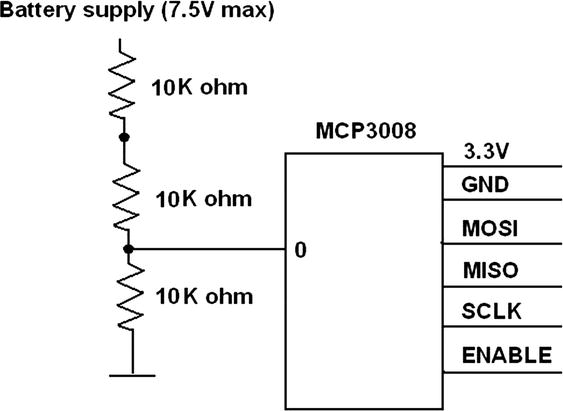
Figure 11-17. Battery monitor schematic

This circuit uses the MCP3008 ADC chip discussed in earlier chapters. You should review the installation and configuration for this chip because it uses SPI, which requires a specialized Python interface library.

The new Behavior subclass is named StopRobot. It implements all three Behavior subsumption methods, as well as one more that sets a real-time voltage level. The following is the class code:

class StopRobot(Behavior):

    critical_voltage = 6.0 # change to any value suitable for robot

    def takeControl(self):
        if self.voltage < critical_voltage:
            return True
        else:
            return False

    def action(self):
        # all stop
        pwmL.ChangeDutyCycle(2.6)
        pwmR.ChangeDutyCycle(2.6)

    def suppress(self):
        # all stop
        pwmL.ChangeDutyCycle(2.6)
        pwmR.ChangeDutyCycle(2.6)

    def setVoltage(self, volts):
        self.voltage = volts

The testBBR class also has to be slightly modified to accept the additional behavior. The following code shows the two statements that must be added to the testBBR class. Notice that the StopRobot behavior is the last one added, making it the highest priority—as it should be.

self.sr = StopRobot() (Add this to the bottom of the list of instantiated Behavior subclasses.)

self.sr.setVoltage(voltage) (Add this right after the voltage measurement.)

python subsumption.py

Summary

Behavior-based robotics (BBR) was this chapter’s theme. BBR is based on animal and insect behavior patterns, especially the ones related to how organisms react to sensory stimulation within their environment.

A brief section discussed how the human brain exhibits multilayer behavioral functions, which range from basic survival behaviors to complex reasoning behaviors. An introduction to the subsumption architecture followed; it is closely modeled after the human brain’s multilayered behavioral model.

Further in-depth discussion went through both simple and complex behavioral models. I choose to use the finite state model (FSM) for this chapter’s robot car demonstration.

I next demonstrated an open source, graphical robotic simulation system named breve. A simple Braitenberg vehicle simulation was created and run that further demonstrated how the stimulus/response behavior pattern functions.

The final demonstration used the Alfie robot car, which was controlled by a Python script created using the subsumption architecture model. The script contained three behaviors, each with its own priority level. I showed how subsumptive-based behavior could take over the robot, depending on the environmental conditions that the robot encountered.