Ambient Light

If you sit in an enclosed room in the daytime, even if your curtains are shut, the room will still be lit because the light will shine through the gaps in the curtains and bounce all over the room. As a result, most of the objects in the room will have roughly the same level of illumination despite none of them being directly illuminated by the sun. Similarly, even shadowed areas on a bright day will appear highly illuminated.

Ambient lighting is our way of approximating global illumination. Generally speaking, methods that model global illumination are computationally expensive because they have to simulate not only the interactions between light sources and objects in the scene but also light bounces between objects and other objects. Ambient light, on the other hand, applies a flat amount of color to every object in the scene to simulate the effect of all those light bounces, particularly light that originated from the sun. Figure 10-1 shows an object illuminated only by ambient light.

A sphere shaded with a gradient of light colours on a dark background.

The amount of ambient light applied to each object is a setting we can manually change at will. If our lighting model only considered ambient light, then the equation to calculate the final color of an object would look like this:

Equation 10-1: Lighting model containing only ambient light

That’s not very interesting so far! It’s worth noting at this point that the light can be any color, so this isn’t just a single floating-point value – it’s an RGB color, just like any other. To build a more interesting model, let’s add different types of direct illumination.

Diffuse Light

A perfectly matte (non-shiny) surface tends to reflect light “evenly” – that is, the amount of reflected light depends on the properties of the surface and the angle between the light and the surface, and a small change in that angle causes a small change in the amount of reflected light. This is called diffuse lighting, which is a type of direct illumination. We use the vector between a point on the object’s surface and the light source, called the light vector and denoted by l, and the normal vector at the same point on the surface, denoted by n, to calculate the amount of diffuse light falling onto an object. Diffuse light is not influenced at all by the position of the viewer (camera) relative to the object or the light source. Figure 10-2 shows the diffuse interaction between the light source and the surface.

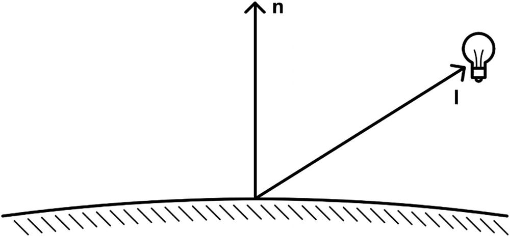
A matte surface with a right-angled normal vector n and light vector l for the calculation of diffused light.

The dot product between n and l gives us the proportion of ambient light acting on the surface. It’s also worth mentioning that these vectors should be normalized prior to any lighting calculation, because that means the result will always be between –1 and 1. Since the dot product can be negative, we clamp negative values to zero; otherwise, we will encounter visual errors. This value is then multiplied by the color of the light source to give us the total diffuse lighting contribution. We can model the diffuse light with the following equation:

Equation 10-2: Diffuse lighting calculation

In Figure 10-3, you’ll see an object lit by both ambient and diffuse light. As you can see, diffuse lighting is characterized by a smooth falloff from a fully lit region, which is directly lit by the light source, to a shadowed region.

A sphere shaded with a gradient of light colours on a dark background. The colours get lighter on the top left of the sphere.

Let’s update our lighting model from Equation 10-1 to include diffuse lighting too. Lighting is additive, so all we need to do to calculate the total amount of lighting acting on the object is to sum the individual types of light.

Equation 10-3: Lighting model containing ambient and diffuse light

Diffuse lighting is perhaps the most noticeable type of lighting, especially when you move the light source or the object. However, there are other types of lighting that depend on the position of the viewer.

Specular Light

When you view a shiny object, the position and strength of the reflective highlight changes whenever you move the object or the angle at which you look at it. This is called specular lighting, and it occurs when the surface of an object is smooth. With diffuse light, the surface typically has imperceptible bumps and other imperfections, which mean reflected light is scattered in all directions. With specular light, on the other hand, all or most of the light rays that reach the object’s surface are reflected at the same angle. This means there is always a part of the surface that strongly reflects many rays directly into the viewer, which is why you see very bright highlights on a small section of the surface.

The amount of specular light is proportional to the dot product between two vectors: the vector between a point on the surface of the object and the viewer, denoted v, and the light ray reflected off the surface, denoted r. The reflected light ray, r, is itself the result of reflecting the incoming light ray, l, in the normal vector, n, which is computationally expensive to calculate. These vectors are shown in Figure 10-4.

An object's surface with a right-angled normal vector n, inclined light vector l, view vector v, and the reflected vector r for the calculation of specular light.

The result of the dot product is raised by a power, α, where a higher power represents a higher degree of shininess. This value is also multiplied by the light color to obtain the final specular light value.

Equation 10-4: Specular lighting

This is computationally expensive to calculate due to the reflection step. A slightly different approach, developed by Jim Blinn in the 1970s, removes the reflection vector calculation and uses a revised approach. Instead, we calculate the half vector between v, the viewer, and l, the light source – this is, comparatively, very easy to compute, so we use this calculation in shaders instead. The half vector is denoted by h, as seen in Figure 10-5.

An object's surface with a normal vector n, inclined light vector l, view vector v, and the half vector h for the calculation of specular light by Blinn’s method.

Then, the specular lighting can be obtained using the dot product between n and h. We still need to raise the result by a power, α, although this method typically requires higher powers for a similar result to the first approach.

Equation 10-5: Specular lighting with Blinn’s modification

With specular lighting, we see a highlight on the object that moves in relation to the light source position and the viewer position. Figure 10-6 shows an object that is lit by ambient, diffuse, and specular lighting. This time, the base color of the object is red so that the specular highlight is easier to see.

A vivid gradient sphere on a dark background. The colors get lighter on the top left of the sphere.

Now that we can calculate specular highlights on our objects, we can add specular lighting to the lighting model.

Equation 10-6: Lighting model containing ambient, diffuse, and specular light

Most basic lighting models would stop here and use only these types of light, but there is another type of light that I am quite fond of including in my shaders, so we will briefly cover it too.

Fresnel Light

When you view objects at a very shallow angle, sometimes they will appear bright. You may have seen this effect before in real life in places like large bodies of clear water or the surface of a polished table. The steeper the angle, the less bright the surface will appear. This is called Fresnel lighting (pronounced like “fruh-nell”). Fresnel light typically isn’t included in many classical lighting models, but I like to include it in many of my shaders, especially if my game uses a stylized aesthetic.

Fresnel lighting is inversely proportional to the angle between the viewer and the surface normal. That means that when you view objects at a grazing angle, the Fresnel effect will be very prominent, but if you view the object face-on, there will be zero Fresnel light. As a result, we can calculate the amount of Fresnel light by taking the dot product between the view vector and the surface normal vector and then subtracting it from 1. Remember that n and v should be normalized before the calculation. These vectors can be seen in Figure 10-7.

An object's surface with a right-angled normal vector n as the view vector v calculates the Fresnel light.

In games, it is common to supply a power, β, to control the influence of Fresnel lighting, like we did for specular lighting. When you increase the power, the Fresnel light gets less prominent. Fresnel light is also multiplied by the light color, just like diffuse and specular light were.

Equation 10-7: Fresnel lighting

If you so choose, your lighting model can include Fresnel lighting in addition to the others.

Equation 10-8: Lighting model containing ambient, diffuse, specular, and Fresnel lighting

In Figure 10-8, you will see one sphere using material that has Fresnel and one that doesn’t. The difference is most noticeable at the edges of the sphere where the angle between the viewer and the surface normal is the greatest.

A pair of vivid gradient spheres on a dark background. The colours get lighter on the top left of the sphere. The sphere on the right has a bright outline.

You should now know the theory behind several types of lighting that interact with the surface of an object. Now let’s look at how to incorporate them into shaders.

Blinn-Phong Reflection Model

The Phong reflection model was developed by Bui Tuong Phong in the mid-1970s to model the way light interacts with the surface of an object, based on the properties of the object itself. It combines ambient, diffuse, and specular lighting to approximate how lighting operates in a real-world scene, as seen in Equation 10-6. The Blinn-Phong reflection model implements Blinn’s alternative calculation of specular lighting into the existing Phong reflection model, as discussed previously. These reflection models work by taking the surface properties of many points on the object’s surface (such as the base color, shininess, and normal vector) and the light vector, view vector, and half vector relative to those points and calculating the final color at each of those points.

Flat shading, Gouraud shading, and Phong shading are three methods for evaluating the amount of light on a surface. Each technique evaluates different locations on the object’s surface and uses different interpolation techniques to obtain the final light amount on each pixel. Let’s see how each of these techniques works.

Flat Shading

Flat shading methods use a single lighting value for each face of the mesh. Since every pixel in a triangle has the same amount of light falling on it, each face of the mesh appears flat, hence the name. To achieve flat shading, all pixels belonging to a particular triangle use the same vectors for the lighting calculations so that the final lighting value is the same for each of those pixels. However, we can still use textures for the base color of the object, so the pixels of a given face can still have different output colors.

We can choose any point on the surface of a triangle to serve as the “basis” point of lighting calculations for the whole triangle, as long as we consistently use the same method for all triangles. Usually, we pick either the first vertex or the centroid (middle point) of the triangle. Also, although the Blinn-Phong model contains specular lighting as a component, it’s usually omitted when using flat shading because specular highlights on objects are typically very small and not captured well with flat shading techniques. Similarly, I will omit Fresnel lighting from the equation for flat shading.

A pair of vivid gradient spheres on a dark background. The surface of the spheres is observed with meshes. The left sphere is smoothened.

Flat shading is a very efficient rendering technique, so it can be used to minimize the performance impact of your game, or when combined with low-poly meshes, flat shading can be used to achieve a stylized aesthetic in your game. Now that we know what flat shading is, let’s see an example of how to use it in both HLSL shader code and Shader Graph. This shader will support basic texture mapping and will tint each triangle of the mesh based on its exposure to the primary directional light present in the scene. For now, this is the only light we will consider.

Flat Shading in HLSL

Let’s create a new HLSL shader called “FlatShading.shader” and remove all its contents. At the top, name the shader “FlatShading” and open a Shader block. I’ve specified a skeleton set of code for this file that we can modify. For most of the shader, there are relatively minor differences between the code for the built-in pipeline and for URP.

Shader "Examples/FlatShading"

{

      Properties { ... }

      SubShader

      {

            Tags

            {

                  "RenderType" = "Opaque"

                  "Queue" = "Geometry"

            }

            Pass

            {

                  Tags { ... }

                  HLSLPROGRAM

                  #pragma vertex vert

                  #pragma fragment frag

                  struct appdata { ... };

                  struct v2f { ... };

                  v2f vert(appdata v) { ... }

                  float4 frag(v2f i) : SV_Target { ... }

                  ENDHLSL

            }

      }

}

Listing 10-1

Code skeleton for the FlatShading shader

Let’s handle the Properties block. We only need to define the surface properties of the mesh here – this isn’t the place to put anything related to the lights in the scene. With that in mind, I’m going to add _BaseColor and _BaseTex properties for now.

Properties

{

      _BaseColor ("Base Color", Color) = (1, 1, 1, 1)

      _BaseTex("Base Texture", 2D) = "white" {}

}

Listing 10-2

The Properties block

Inside the HLSLPROGRAM block, we must declare those properties again. The code is slightly different between the built-in pipeline and URP because we must conform to the SRP Batcher rules in URP. Put the following lines of code for the pipeline you are using between the v2f struct definition and the vert function.

struct v2f { ... };

sampler2D _BaseTex;

float4 _BaseColor;

float4 _BaseTex_ST;

Listing 10-3

Declaring properties in HLSL in the built-in pipeline

struct v2f { ... };

sampler2D _BaseTex;

CBUFFER_START(UnityPerMaterial)

      float4 _BaseColor;

      float4 _BaseTex_ST;

CBUFFER_END

Listing 10-4

Declaring properties in HLSL in URP

Now let’s look at the appdata and v2f structs. The appdata struct will take in the object-space position of each vertex, as well as a set of UV coordinates. We also require the normal vector for the lighting calculations, which comes with its own shader semantic, NORMAL. These normals are in object space, so I’ll call the variable normalOS.

struct appdata

{

      float4 positionOS : POSITION;

      float2 uv : TEXCOORD0;

      float3 normalOS : NORMAL;

};

Listing 10-5

The appdata struct

The normalOS input takes the normal vectors attached to each vertex of the mesh and automatically uploads them to the shader for us to use.

The v2f struct requires the clip-space position and the UVs to be passed to the fragment shader. Since we are using flat shading, we can calculate all the lighting inside the vertex shader and send it to the fragment shader inside the v2f struct, so we won’t need to also include the normal vector in v2f. However, flat shading requires us to only calculate the lighting once per triangle so we must prevent the lighting value being interpolated between each vertex of the triangle using the nointerpolation keyword. There is no special semantic to use for lighting values, so we’ll just use the next available general-use interpolator, which is TEXCOORD1.

Note

Remember that TEXCOORD0, TEXCOORD1, and so on are known as “interpolators.” However, this doesn’t mean their values must be interpolated (mixed) between vertices. Shader terminology can often be confusing! The nointerpolation keyword prevents interpolation from taking place, which means the result from the first vertex of each triangle is used in the v2f struct and sent to every fragment for that triangle.

struct v2f

{

      float4 positionCS : SV_POSITION;

      float2 uv : TEXCOORD0;

      nointerpolation float4 flatLighting : TEXCOORD1;

};

Listing 10-6

The v2f struct

The flatLighting value inside v2f will contain the final light color that we can apply to objects inside the fragment shader. The fragment shader is identical in the built-in pipeline and URP, so let’s handle it before discussing the vertex shader. All we need to do is sample _BaseTex and multiply by _BaseColor like usual, but now we have a flatLighting value to multiply by too.

float4 frag (v2f i) : SV_Target

{

      float4 textureSample = tex2D(_BaseTex, i.uv);

      return textureSample * _BaseColor * i.flatLighting;

}

Listing 10-7

The fragment shader

Finally, let’s handle the vertex shader, which will be doing most of the heavy lifting for this shader. The code we’ll use to access lighting information differs wildly between the built-in pipeline and URP, so let’s deal with both versions separately.

Accessing Lights in the Built-In Pipeline

First, let’s deal with some built-in pipeline specifics. We should specify that we are using forward rendering by supplying a LightMode tag called ForwardBase. This goes inside a new Tags block inside the Pass, rather than the existing Tags block that is inside the SubShader.

Pass

{

      Tags

      {

            "LightMode" = "ForwardBase"

      }

      ...

Listing 10-8

Using the ForwardBase LightMode in the built-in pipeline

Unity supplies a few helpful variables that we can use for lighting inside a file called “Lighting.cginc”. We can include this file near the top of the HLSLPROGRAM block alongside the UnityCG.cginc file.

HLSLPROGRAM

#pragma vertex vert

#pragma fragment frag

#include "UnityCG.cginc"

#include "Lighting.cginc"

...

Listing 10-9

Including Lighting.cginc and UnityCG.cginc in the built-in pipeline

With that out of the way, we can move to the vert function. As with most vertex shaders, we must convert object-space positions to clip-space positions (which requires different functions between the built-in pipeline and URP), and since we’re using textures, we must also pass the UV coordinates through. Here’s a skeleton for the vert function in the built-in pipeline and in URP.

v2f vert (appdata v)

{

      v2f o;

      o.positionCS = UnityObjectToClipPos(v.positionOS.xyz);

      o.uv = TRANSFORM_TEX(v.uv, _BaseTex);

      ...

      return o;

}

Listing 10-10

The vert function skeleton in the built-in pipeline

Our calculations require the world-space normal vector, but we passed object-space normals to the vert function through appdata. We can convert from object to world space using the UnityObjectToWorldNormal function, which is included in UnityCG.cginc.

o.uv = TRANSFORM_TEX(v.uv, _BaseTex);

float3 normalWS = UnityObjectToWorldNormal(v.normalOS);

Listing 10-11

Converting from object- to world-space normals

Next, we will calculate the amount of ambient lighting acting upon the object. Unity makes the ambient light and the result from light probes available in the form of spherical harmonics coefficients. You don’t need to know the specifics behind this – we just need to know that the ShadeSH9 function can be used to obtain the ambient light, which includes light contributions from the skybox, as well as light probes.

float3 normalWS = UnityObjectToWorldNormal(v.normalOS);

float3 ambient = ShadeSH9(half4(normalWS, 1));

Listing 10-12

Ambient lighting in the built-in pipeline

The diffuse lighting comes next. We can access the color of the primary directional light with the _LightColor0 variable, defined in Lighting.cginc, as well as its direction with the _WorldSpaceLightPos0 variable. Since it is a directional light, the positioning of the light relative to the object doesn’t matter. Once we have those values, we can use Equation 10-2 to calculate the amount of diffuse light.

Note

The name _WorldSpaceLightPos0 might be confusing because it’s called “pos” but it’s getting the light direction in this example. Essentially, this variable contains details about the most prominent light in the scene. That’s usually a directional light, in which case the variable returns its direction. If it is a different type of light, like a point light, this variable does indeed contain its position in world space.

float3 ambient = ShadeSH9(half4(normalWS, 1));

float3 diffuse = _LightColor0 * max(0, dot(normalWS, _WorldSpaceLightPos0.xyz));

Listing 10-13

Diffuse lighting with one directional light in the built-in pipeline

Now all that’s left is to combine each component of the lighting into a single value to be included in the v2f struct.

      float3 diffuse = _LightColor0 * max(0, dot(normalWS, _WorldSpaceLightPos0.xyz));

      o.flatLighting = float4(ambient + diffuse, 1.0f);

      return o;

}

Listing 10-14

Adding together lighting components in the built-in pipeline

You should now see flat shading in objects in your scene that look just like Figure 10-9. Now let’s see how to do all this in URP instead.

Accessing Lights in URP

Let’s deal with a few URP specifics before jumping into the vert function. Since we are using URP, we need to add a RenderPipeline tag specified as such in the Tags block inside the SubShader.

SubShader

{

      Tags

      {

            "RenderType" = "Opaque"

            "Queue" = "Geometry"

            "RenderPipeline" = "UniversalPipeline"

      }

      ...

Listing 10-15

Specifying URP inside the Tags block in the SubShader

Then, inside the Tags block in the Pass, we will be using the UniversalForward LightMode.

Pass

{

      Tags

      {

            "LightMode" = "UniversalForward"

      }

      ...

Listing 10-16

Using UniversalForward in URP

In URP, many lighting helper functions are provided for us inside a file called “Lighting.hlsl”, which we will use extensively throughout the remaining portions of the code. We can include it alongside the Core.hlsl file inside the HLSLPROGRAM block near the top.

HLSLPROGRAM

#pragma vertex vert

#pragma fragment frag

#include "Packages/com.unity.render-pipelines.universal/ShaderLibrary/Core.hlsl"

#include "Packages/com.unity.render-pipelines.universal/ShaderLibrary/Lighting.hlsl"

...

Listing 10-17

Including Core.hlsl and Lighting.hlsl

As we did with the built-in pipeline example, let’s create a skeleton vert function that transforms positions from object to clip space and passes UV coordinates onto the frag function.

v2f vert (appdata v)

{

      v2f o;

      o.positionCS = TransformObjectToHClip(v.positionOS.xyz);

      o.uv = TRANSFORM_TEX(v.uv, _BaseTex);

      ...

      return o;

}

Listing 10-18

The vert function skeleton in URP

The remaining code slots in place of the ellipsis in this skeleton code snippet. First, we must convert the normal vectors to world space using the TransformObjectToWorldNormal function.

o.uv = TRANSFORM_TEX(v.uv, _BaseTex);

float3 normalWS = TransformObjectToWorldNormal(v.normalOS);

Listing 10-19

Object- to world-space calculation for normals

Next, we can calculate the amount of ambient light acting upon the object. This requires us to sample the spherical harmonics coefficients like we did in the built-in pipeline example, except this time the function is called SampleSHVertex and it requires the world-space normal as a float3. There is a corresponding function called SampleSHPixel that is intended for the fragment shader, but we won’t need it here.

float3 normalWS = TransformObjectToWorldNormal(v.normalOS);

float3 ambient = SampleSHVertex(normalWS);

Listing 10-20

Ambient lighting in URP

Next, we’ll get the diffuse light contribution. We can access information about the main light using the GetMainLight function, which is included in Lighting.hlsl. It returns a Light object, which contains several helpful bits of information that we’ll use to help calculate the lighting on our objects, such as its color and direction. We’ll calculate the amount of diffuse light using Equation 10-2.

float3 ambient = SampleSHVertex(normalWS);

Light mainLight = GetMainLight();

float3 diffuse = mainLight.color * max(0, dot(normalWS, mainLight.direction));

Listing 10-21

Diffuse lighting with one directional light in URP

Finally, we can add together each component of the light to obtain a value to pass to the fragment shader. We’re only using ambient and diffuse lighting for flat shading, so those are the two values we’ll add. The flatLighting variable is a float4, so we’ll need to fill in the last component with a 1.

      float3 diffuse = mainLight.color * max(0, dot(normalWS, mainLight.direction));

      o.flatLighting = float4(ambient + diffuse, 1.0f);

      return o;

}

Listing 10-22

Adding together lighting components

With that, you should now see flat shading just like in Figure 10-9 in your scene. We have now seen how flat shading works in shader code, so let’s move on to Shader Graph and see how we can implement flat shading there.

Flat Shading in Shader Graph

This graph is going to look a bit different from the ones we’ve made so far. In previous examples, each graph we have seen has been an Unlit graph, which means Unity does not automatically apply lighting to the object. However, now that we’re starting to incorporate lighting into our shaders, it’s time to start thinking about Shader Graph’s Lit option. Let’s create a new Lit graph and name it “FlatShading.shadergraph”.

You should see two key differences. First, the master stack will contain several never-before-seen blocks. Second, the Graph Settings tab will have a few extra options in it, as seen in Figure 10-10.

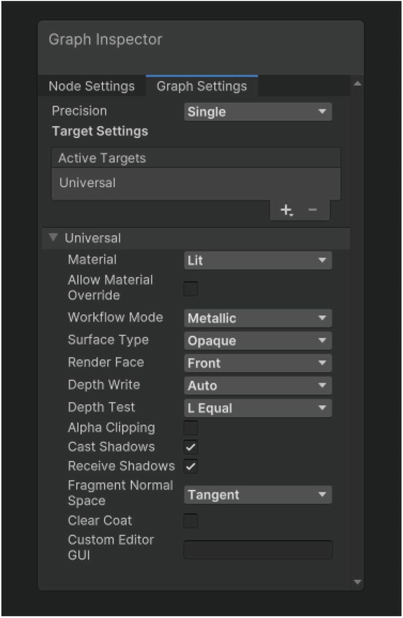
A screenshot of a graph inspector window lists the precision, target, and universal settings under the graph settings tab with fragment and vertex nodes.

A Lit shader applies the lighting model automatically to objects, but instead of using the Blinn-Phong lighting model we’ve discussed previously, it uses Physically Based Rendering (PBR). We will explore PBR lighting later in this chapter, but for now we will focus on getting the flat shading effect to work. It is a lot of work to get true Blinn-Phong lighting to work inside Shader Graph, and it’s a little bit overkill for this effect, so for now, we will implement flat shading using PBR. The upshoot is that the only thing we need to modify is the normal vector output in the Fragment section of the master stack. By replacing the normal vector, which by default is a per-pixel normal vector that has been interpolated across the surface of the mesh, with a per-triangle normal vector, which we can calculate, we’ll end up with the flat shading we desire.

Here's how to do that. First, the graph requires Base Color and Base Texture properties, so I will include those on the Blackboard with the values seen in Figure 10-11 and wire them up to the Base Color output of the graph, as seen in Figure 10-12.

A screenshot of property boxes of base texture and base color with fields as: name, reference, default, mode, precision, exposed, override property, and declaration.

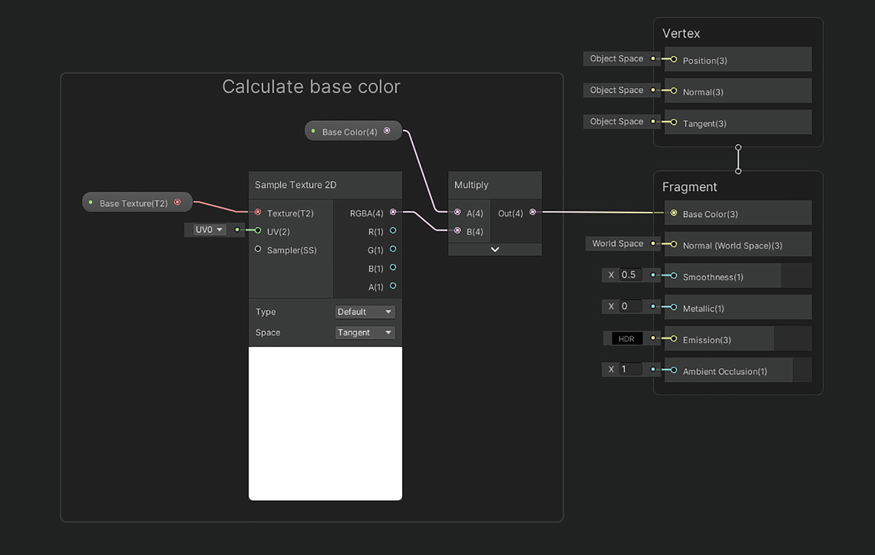
A screenshot of a dark screen illustrates how the base color and the parameters of sample texture 2 D are multiplied and the output is fragmented as the base color.

Now we’ll calculate the new normals. We don’t have access to anything like the nointerpolation modifier that we used in HLSL code, so we must calculate the per-triangle normal vector ourselves inside the fragment stage. In this stage of rendering, the shader has no knowledge of where the other vertices of the triangle are, so we can’t just calculate the normals based on that information. However, we do know that any triangle face is always flat, and we can exploit that fact. The ddx and ddy functions in shaders, which are called partial derivative functions, can be used to calculate any input on the current pixel and an adjacent pixel (horizontally for ddx and vertically for ddy) to obtain two values and then return the difference between them. The equivalent nodes in Shader Graph are called DDX and DDY.

For example, if we input the world-space position to the ddx and ddy functions, we would obtain two small vectors, perpendicular to each other, that lie on the triangle’s surface. The shrewd among you may have realized we can use the cross product on both those vectors to obtain the normal vector pointing away from the triangle, which is exactly what we wanted. The nice thing about this calculation is that, because the triangle is flat, we obtain the same normal vector for each pixel of the triangle, which results in a flat-shaded object. We just have to be careful with the order in which we use the two values with the cross product – the ddy comes first and then ddx.

This normal vector value is in world space. In Figure 10-10, you’ll see that the Fragment stage Normal output, by default, expects a tangent-space vector, so we’ll need to do a small modification. If we go into the Graph Settings (also seen in Figure 10-10), you’ll notice the Fragment Normal Space option, which we can change to World, so that Unity swaps out the tangent-space Normal block with a world-space Normal block. If we take the result of the Cross Product node, pass it through a Normalize node, and output it to the Normal (World Space) block, we’ll get the flat shading we desire. Figure 10-13 shows how these nodes are connected to each other.

A screenshot of a dark screen illustrates how positions of the sample mesh for each triangle are multiplied and the normalized output is fragmented as the base color.

This technique allows us to generate per-triangle normals in Shader Graph, but this is far more expensive than the HLSL equivalent, because rather than calculating them once for each triangle and passing that value to each fragment for the lighting calculations like HLSL does, in Shader Graph we must recalculate the normal vector for each fragment, which includes an expensive cross product calculation. However, it’s not so prohibitively expensive that you would notice a significant slowdown in your game using this method.

You now know how to implement flat shading into your game, no matter whether you are using HLSL code or Shader Graph. Next, let’s look at another type of shading: Gouraud shading.

Gouraud Shading

Gouraud shading is a technique that was developed in the early 1970s by Henri Gouraud. With Gouraud shading, the amount of light is evaluated at every vertex of an object and interpolated between those vertices to obtain lighting values for each pixel, as seen in Figure 10-14.

A vivid gradient sphere on a dark background. The colors get lighter on the top left of the sphere which has a hexagonal shape.

The advantage of Gouraud shading over flat shading is that we get a lighting gradient between each vertex due to the use of interpolation and we can implement specular lighting now. However, it’s slightly more resource-intensive than flat shading, and specular lighting still suffers from severe artifacts that can be avoided by using a high-poly object to obtain higher-“resolution” reflections. That introduces problems of its own, however – when we cover Phong shading, we’ll see that subdividing the geometry is unnecessary. But we’re getting ahead of ourselves – let’s see how Gouraud shading works in shader code and then in Shader Graph.

Note

The Gouraud shading effect is interesting as a curiosity or if you are explicitly going for a retro 3D look for your game, but otherwise, you will probably want to use Phong shading instead, which I cover next.

Gouraud Shading in HLSL

We’ll start by creating a new shader file and naming it “GouraudShading.shader”. Here’s the skeleton for this shader.

Shader "Examples/GouraudShading"

{

      Properties { ... }

      SubShader

      {

            Tags

            {

                  "RenderType" = "Opaque"

                  "Queue" = "Geometry"

            }

            Pass

            {

                  Tags { ... }

                  HLSLPROGRAM

                  #pragma vertex vert

                  #pragma fragment frag

                  struct appdata

                  {

                        float4 positionOS : POSITION;

                        float2 uv : TEXCOORD0;

                        float3 normalOS : NORMAL;

                  };

                  struct v2f { ... };

                  v2f vert(appdata v) { ... }

                  float4 frag(v2f i) : SV_Target { ... }

                  ENDHLSL

            }

      }

      Fallback Off

}

Listing 10-23

Skeleton code for the GouraudShading shader

Many parts of this shader are different from the FlatShading shader, so let’s start with the Properties block. In addition to the _BaseColor and _BaseTex properties that we previously saw, we need a property to control the glossiness of the object. With Gouraud shading, we will be including the specular lighting component and raising it by a power. Therefore, we will add a _GlossPower property.

Properties

{

      _BaseColor ("Base Color", Color) = (1, 1, 1, 1)

      _BaseTex("Base Texture", 2D) = "white" {}

      _GlossPower("Gloss Power", Float) = 400

}

Listing 10-24

Gouraud shading properties

We need to declare these within the HLSLPROGRAM block between the v2f struct and the vert function – the syntax is slightly different between the built-in pipeline and URP.

struct v2f { ... };

sampler2D _BaseTex;

float4 _BaseColor;

float4 _BaseTex_ST;

float _GlossPower;

Listing 10-25

Declaring properties in the built-in pipeline

struct v2f { ... };

sampler2D _BaseTex;

CBUFFER_START(UnityPerMaterial)

      float4 _BaseColor;

      float4 _BaseTex_ST;

      float _GlossPower;

CBUFFER_END

Listing 10-26

Declaring properties in URP

The appdata struct is the same as the FlatShading shader – we need the object-space position and UVs like most of our shaders, plus the object-space normals. The v2f struct, on the other hand, looks a bit different. The lighting calculation will be more complicated because we’re including the specular component. Typically, the ambient and diffuse light end up being multiplied by the object’s base color, but the specular highlight does not. That means we can’t just send the total light to the fragment shader inside a single variable in v2f like we did in the FlatShading shader – we’ll need to split it into two parts. With that in mind, we’ll include the clip-space position and the UVs in v2f as we would with a typical shader. Plus, we’ll include the ambient and diffuse light inside a variable called diffuseLighting and the specular component in a variable called specularLighting.

struct v2f

{

      float4 positionCS : SV_POSITION;

      float2 uv : TEXCOORD0;

      float4 diffuseLighting : TEXCOORD1;

      float4 specularLighting : TEXCOORD2;

};

Listing 10-27

The v2f struct with split lighting components

Let’s jump ahead to the fragment shader and incorporate those variables now. The frag function is fairly simple, as all we need to do is sample _BaseTex and multiply it by _BaseColor and diffuseLighting. Then we can add the specularLighting to obtain the final color of the object.

float4 frag (v2f i) : SV_Target

{

      float4 textureSample = tex2D(_BaseTex, i.uv);

      return textureSample * _BaseColor * i.diffuseLighting + i.specularLighting;

}

Listing 10-28

Fragment shader adding diffuse and specular lighting contributions

Now we come to the vertex shader, where most of the calculations take place. The code is very different between the built-in pipeline and URP, so I’ll split the rest of the example into two sections.

Gouraud Vertex Shader in the Built-In Pipeline

The vertex shader is more complex than the FlatShading example because we’re including the specular component and splitting the light contributions into two parts before sending them to the fragment shader in the v2f struct. We need to make a few additions to the shader as we saw in Listings 10-8 and 10-9. Then we’ll start the vert function with the same skeleton we saw in Listing 10-10. Then we’ll calculate the vectors we need for subsequent calculations. We need the world-space normals like we did with the FlatShading shader. Plus, we will be using the world-space view vector. Recall that the view vector is the vector between a point on the surface and the camera. Unity provides the WorldSpaceViewDir function for this purpose, which takes the object-space position as a parameter. This vector needs to be normalized.

v2f vert (appdata v)

{

      v2f o;

      o.positionCS = UnityObjectToClipPos(v.positionOS);

      o.uv = TRANSFORM_TEX(v.uv, _BaseTex);

      float3 normalWS = UnityObjectToWorldNormal(v.normalOS);

      float3 viewWS = normalize(WorldSpaceViewDir(v.positionOS));

Listing 10-29

Calculating vectors required for Gouraud shading in the built-in pipeline

Next come the ambient light and diffuse light calculations, which we can copy from Listings 10-12 and 10-13. After that we’ll do the specular light calculation. We first need to calculate the half vector, which we can do by adding the view and light vectors together and normalizing the result. This works because both those vectors are normalized to begin with, so this has the same outcome as adding both and dividing by their combined length. Using the half vector, we can carry out the n-dot-h calculation that Blinn discovered and then raise it to the power of _GlossPower, before multiplying by the light color.

float3 viewWS = normalize(WorldSpaceViewDir(v.positionOS));

float3 ambient = ShadeSH9(half4(normalWS, 1));

float3 diffuse = _LightColor0 * max(0, dot(normalWS, _WorldSpaceLightPos0.xyz));

float3 halfVector = normalize(_WorldSpaceLightPos0 + viewWS);

float specular = max(0, dot(normalWS, halfVector)) * diffuse;

specular = pow(specular, _GlossPower);

float3 specularColor = _LightColor0 * specular;

Listing 10-30

Half vector and specular lighting calculations in the built-in pipeline

The last thing we do in the vertex shader before returning is to set the value of diffuseLighting and specularLighting inside the v2f struct, ready for use in the fragment shader.

      float3 specularColor = _LightColor0 * specular;

      o.diffuseLighting = float4(ambient + diffuse, 1.0f);

      o.specularLighting = float4(specularColor, 1.0f);

      return o;

}

Listing 10-31

Setting diffuseLighting and specularLighting values

All the parts of the vertex shader are in place now, so the shader is complete for the built-in pipeline, and you will see Gouraud shading as in Figure 10-14 on your objects. Let’s see how to write the vertex shader in URP.

Gouraud Vertex Shader in URP

The URP version of this shader needs to include the additions seen in Listings 10-15, 10-16, and 10-17. As with the built-in pipeline example, the URP version of the vertex shader now needs to include specular calculations. Starting with the vertex shader code skeleton from Listing 10-18, let’s calculate the view vector. This uses a different function from the built-in pipeline: this time, the GetWorldSpaceNormalizedViewDir function is the one we want. This takes in a world-space vertex position as a parameter (whereas the built-in pipeline equivalent took an object-space position), so we’ll also have to calculate that first.

v2f vert (appdata v)

{

      v2f o;

      o.positionCS = TransformObjectToHClip(v.positionOS.xyz);

      o.uv = TRANSFORM_TEX(v.uv, _BaseTex);

      float3 normalWS = TransformObjectToWorldNormal(v.normalOS);

      float3 positionWS = mul(unity_ObjectToWorld, v.positionOS);

      float3 viewWS = GetWorldSpaceNormalizeViewDir(positionWS);

Listing 10-32

Calculating vectors required for Gouraud shading in URP

The ambient light and diffuse light calculations are identical to the ones from the FlatShading shader in Listings 10-20 and 10-21. Then we come to the specular lighting calculations. The code for this is almost identical to Listing 10-30, except we use the mainLight variable in URP to access lighting information. We can round off the shader by passing the diffuseLighting and specularLighting values to the fragment shader through the v2f struct.

      float3 ambient = SampleSHVertex(normalWS);

      Light mainLight = GetMainLight();

      float3 diffuse = mainLight.color * max(0, dot(normalWS, mainLight.direction));

      float3 halfVector = normalize(mainLight.direction + viewWS);

      float specular = max(0, dot(normalWS, halfVector));

      specular = pow(specular, _GlossPower);

      float3 specularColor = mainLight.color * specular;

      o.diffuseLighting = float4(ambient + diffuse, 1.0f);

      o.specularLighting = float4(specularColor, 1.0f);

      return o;

}

Listing 10-33

Half vector, specular lighting, and v2f lighting variables in URP

The main differences between this and the built-in pipeline version of the shader are just a matter of different function and variable names, but the resulting visuals (as in Figure 10-14) should be almost identical. Let’s see how this effect can be made in Shader Graph now.

Gouraud Shading in Shader Graph

Implementing Gouraud shading in Shader Graph entails more work than doing the same thing in HLSL. In fact, per-vertex lighting is impossible to achieve in Shader Graph versions prior to 12.0 (Unity 2021.2) because we only have access to three interpolators in the vertex stage: the Position, Normal, and Tangent vectors. With Shader Graph 12.0, we get access to custom interpolators that let us funnel custom data from the vertex stage to the fragment stage, like how the v2f struct in shader code gives us full control over the data passed between the vert and frag functions.

Note

Although I claim it’s impossible, you probably can implement per-vertex lighting in older versions of Shader Graph. However, it will require “hacky” ways of getting round Shader Graph’s limitations and will probably require injecting a lot of code using the Custom Function node, so it’s de facto impossible using the intended behavior of Shader Graph. Regrettably, that means the GouraudShading effect only works in Shader Graph 12.0 (Unity 2021.2) and above.

Another roadblock we will encounter is the fact that Shader Graph does not yet have a built-in node that grabs lighting data such as position, direction, and color from the main light or any additional lights. Therefore, we will need to create a Custom Function node to obtain that information, for which we need to write a short section of shader code. Apologies to anyone wishing to avoid code entirely! We’ll wrap that function inside a Sub Graph so that it’s easy to access this behavior in any future graph that requires it. Using that Sub Graph, we can carry out the diffuse and specular lighting calculations required for the shader.

Note

A built-in Get Main Light node, or equivalent, has been “under consideration” by Unity for a while now. One day it might be available in the base Shader Graph package for URP! In lieu of this node, as of the writing of this book, a Get Main Light Direction node is available in Shader Graph 13.0 (for Unity 2022.1) and up. You still won’t have access to the light color or shadowing, but it’s a start.

GetMainLight Sub Graph

Let’s do this step by step. First, I’m going to write a shader file containing the code to access the lighting information. Then, I’ll create a Sub Graph with relevant inputs and outputs that we will be able to use in any graph that requires lighting information. Finally, I’ll create a Custom Function node inside that Sub Graph, which accesses the custom HLSL code, and wire up the Sub Graph inputs and outputs to that node.

Start by creating a new file called “GetMainLight.hlsl”. Unfortunately, there’s no easy way to create a basic text file from within the Unity Editor, so you’ll have to do this in an external text editor or IDE such as Visual Studio. This file will contain one function. Recall from all the way back in Chapter 4 that Custom Function nodes require a particular syntax for the function:

• We need to put the variable precision at the name after an underscore, that is, FunctionName_float or FunctionName_half.

• We put all the input and output variables inside the parameter list in the function signature:

  • Inputs look like any regular function parameter (such as “float3 input”).

  • Outputs use the out keyword (such as “out float3 output”).

• The function uses the void return type.

With that in mind, I’ll write a function that returns similar information to the GetMainLight function that already exists in HLSL for URP. I’ll use float precision for each variable, so with that in mind, here’s the function signature.

void MainLight_float(float3 WorldPos, out float3 Direction, out float3 Color,

      out float DistanceAtten, out float ShadowAtten)

{

      ...

}

Listing 10-34

GetMainLight custom function signature

This function takes the world-space position as input and outputs the direction, color, distance attenuation, and shadow attenuation of the main light at that position. In almost every case, the main light will be a directional light. We won’t need the last two outputs just yet, but we’ll include them here for completeness.

The first wrinkle we’ll encounter is that Shader Graph is able to preview the output of any node inside a tiny window on the node itself, but that preview window doesn’t have access to any lights, so we’ll have to account for that in our code. We can use #ifdef SHADERGRAPH_PREVIEW to check if the code is being run inside a Shader Graph preview window, and if so, we’ll return dummy values that simulate a white directional light.

void MainLight_float(float3 WorldPos, out float3 Direction, out float3 Color,

 out float DistanceAtten, out float ShadowAtten)

{

#ifdef SHADERGRAPH_PREVIEW

      Direction = normalize(float3(0.5f, 0.5f, 0.25f));

      Color = float3(1.0f, 1.0f, 1.0f);

      DistanceAtten = 1.0f;

      ShadowAtten = 1.0f;

#else

      ...

#endif

}

Listing 10-35

Dummy values for inside a Shader Graph preview window

Otherwise, the code is being run for real, and we’ll need to access real values. We can use the very same GetMainLight function that we used in the HLSL version of this shader, except this time I’ll pass shadow coordinates to the function that we can obtain using the TransformWorldToShadowCoord function. Don’t worry too much about this just yet – we will discuss shadows later in the chapter. Using the Light object that is returned by GetMainLight, we can access the values we need for the function’s outputs.

#else

      float4 shadowCoord = TransformWorldToShadowCoord(WorldPos);

      Light mainLight = GetMainLight(shadowCoord);

      Direction = mainLight.direction;

      Color = mainLight.color;

      DistanceAtten = mainLight.distanceAttenuation;

      ShadowAtten = mainLight.shadowAttenuation;

#endif

Listing 10-36

Using GetMainLight inside a custom function

That’s all we need to do for the code. Let’s now create the Sub Graph that will contain the Custom Function node that uses this code – name it “GetMainLight.shadersubgraph”. You’ll see an interface similar to a main graph, except the output stack will contain only a single float4 output by default. The first thing we’ll do is set up the inputs and outputs of the Sub Graph.

The inputs to a Sub Graph work the same as the properties of a main graph, so we’ll add a Vector3 input called WorldPos to the graph using the Blackboard window. The default value can be left as (0,0,0). The outputs are slightly different. If you click the Output node, which is exclusive to Sub Graphs, you will be able to add more outputs in the Node Settings window. Use the plus arrow to add more outputs, click any of the names to edit them, and use the type drop-down to change the type of the output. Wire up the outputs to match those used in the HLSL function we wrote, as seen in Figure 10-15.

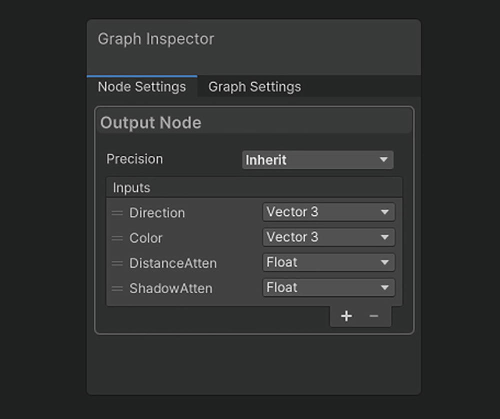
A graph inspector window lists the options under the node settings tab that has output node parameters of precision and inputs as: Direction, Color, Distance Atten, and Shadow Atten.

Now that the inputs and outputs are sorted, let’s add a Custom Function node to the graph. Similarly, we need to set up inputs and outputs to the function, which can all be done in the Node Settings. We also need to specify which HLSL function the node will be using. We do this by attaching the GetMainLight.hlsl file to the File slot and then typing in the name of the function without the precision suffix – in our case, we called it “MainLight”. Figure 10-16 shows how the inputs, outputs, and file attachments should look in the Node Settings.

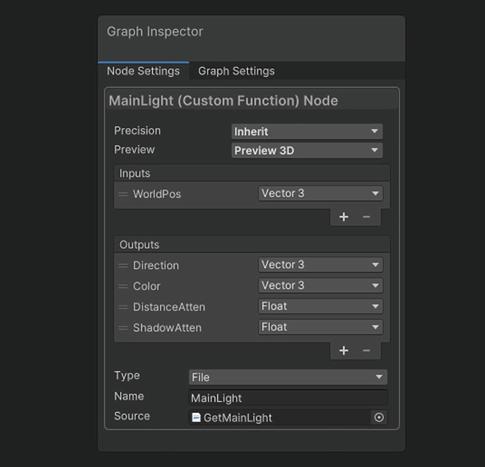
A graph inspector window lists options under the node settings tab as: precision, preview, inputs, outputs, type, name, and source.

Then we can wire up the Sub Graph inputs to the Custom Function node inputs and the Sub Graph outputs to the Custom Function node outputs, as seen in Figure 10-17.

A screenshot of a dark screen illustrates how parameters of the main light functions such as direction, color, Distance Atten, and Shadow Atten are mapped to the output.

If you get red errors on the Custom Function node, you might need to go into the Graph Settings and change the Precision of the graph to Single. We can now use main light information in our graphs, which will be enough for the diffuse and specular lighting, but we still need to handle ambient light. We can use the same process to create a Sub Graph just for ambient light too. Although Shader Graph ships with an Ambient node, this only exposes three modes of ambient light – sky, equator, and ground – none of them work as well as the method we used in the HLSL version of the shader, so we’re going to use the same code here.

GetAmbientLight Sub Graph

Since we’ve already seen much of this process at work, let’s speed through this section. We’ll create a new file called “GetAmbientLight.hlsl” in an external text editor and place the following code inside it.

void AmbientLight_float(float3 WorldNormal, bool IsVertex, out float3 Ambient)

{

#ifdef SHADERGRAPH_PREVIEW

      Ambient = 0.2f;

#else

      if(IsVertex)

      {

            Ambient = SampleSHVertex(WorldNormal);

      }

      else

      {

            Ambient = SampleSH(WorldNormal);

      }

#endif

}

Listing 10-37

GetAmbientLight function

The SampleSH and SampleSHVertex functions require the world-space normal as a parameter. I also added a Boolean switch to choose whether we want to calculate the ambient lighting per vertex or per fragment. Then follow these steps to set up the Sub Graph:

• Create the Sub Graph by right-clicking the Project View and choosing Create ➤ Shader ➤ Sub Graph and naming it “GetAmbientLight”.

• Add a Custom Function node to the graph and change the File option to GetAmbientLight.hlsl and the Function option to “AmbientLight”.

• Create a WorldNormal Vector3 input and an IsVertex Boolean input for both the Sub Graph and the Custom Function node.

• Create an Ambient Vector3 output for both the Sub Graph and the Custom Function node.

• Connect the input nodes and Output node to the Custom Function node as required.

The resulting graph should look like Figure 10-18.

A screenshot of a dark screen illustrates how the parameters of the ambient light functions such as world normal, is vertex, and ambient are mapped to the output.

These Sub Graphs can now be used in any future graph that requires access to either main light or ambient light information. Without further ado, let’s write a graph that can perform Gouraud shading.

Gouraud Shading with Custom Interpolators

Start by creating a new Unlit graph. This time, we’re going back to an Unlit graph so that we can perform the lighting calculations ourselves in the vertex stage and avoid Unity applying a second layer of lighting to the object automatically. Name this graph “GouraudShading.shadergraph”.

First, we’ll set up the properties required for the graph. It requires three properties: a Color called Base Color, a Texture2D called Base Texture, and a Float called Gloss Power. These will work similarly to those we used in the HLSL version of the shader, and you can see them in Figure 10-19.

A dark screen lists the base texture, base color, and gloss power for the Gouraud Shading graph that has a name, reference, default, mode and override property declaration.

We will be doing the lighting calculations in the vertex shader and will need to pass them to the fragment shader. To do this, we need to make use of Shader Graph’s custom interpolator feature. If you right-click inside the Vertex section of the master stack and choose Add Block Node, a Custom Interpolator option will show up. Add two of those and name them “DiffuseLighting” and “SpecularLighting”, respectively, in the Node Settings. Both use the Vector3 type.

For the diffuse lighting, we’ll carry out the following calculations:

• Perform the Dot Product between the Normal Vector and the Direction output of GetMainLight to obtain the amount of diffuse light.

• Saturate the result to remove any negative results.

• Multiply by the Color output of GetMainLight to tint the diffuse light with the main light’s color.

• Add the GetAmbientLight result to the diffuse light.

• Output the result to the DiffuseLighting custom interpolator on the master stack’s Vertex section.

A dark screen illustrates how diffuse and ambient lighting are calculated by the dot product of the normal vector and Get Main Light.

And for the specular lighting, we’ll carry out these calculations:

• Add the View Vector and the Direction output of GetMainLight together and then Normalize the result to obtain the half vector.

• Take the Dot Product between the Normal Vector and that half vector to obtain the amount of specular light.

• Saturate the result to remove any negative results.

• Raise the result to the power of the Gloss Power property using a Power node.

• Multiply by the Color output of GetMainLight to tint the specular light with the main light’s color.

• Output the result to the SpecularLighting custom interpolator on the master stack’s Vertex section.

A dark screen illustrates how specular lighting is calculated from normalized view vector and Get Main Light and is saturated and multiplied with gloss power to get the desired outcome.

Now let’s combine these types of light in the fragment stage. We can access the resulting values from the custom interpolators in the fragment stage using the DiffuseLighting and SpecularLighting nodes, respectively, as follows:

• Sample the Base Texture with a Sample Texture 2D node and multiply the output by Base Color.

• Multiply the result by the DiffuseLighting custom interpolator value.

• Add the SpecularLighting custom interpolator value.

• Output the result to the Base Color output on the master stack’s fragment section.

A dark screen illustrates how base color and lighting are calculated from the product of base texture and diffuse lighting and are added with specular lighting to get the base color.

With those steps followed, you’ll see a result just like in Figure 10-14. This is a relatively complicated graph, so the nodes might be hard to see all on-screen at once! Now that we have seen how Gouraud shading works in both HLSL and Shader Graph, let’s see how Phong shading improves on Gouraud shading.

Phong Shading

First, let’s clarify what we mean by Phong shading. We’ve talked about the Phong reflection model, where we add ambient, diffuse, and specular contributions at different points to calculate the amount of light incident on an object’s surface. Phong shading is a different thing, but annoyingly we use the same terminology, which is often conflated.

Phong shading is an interpolation technique. With Gouraud shading, we calculated lighting per vertex and interpolated the result across fragments. With Phong shading, we instead interpolate the normal vector and view vector across fragments, renormalize them, and then calculate lighting per fragment. This technique is much more expensive than Gouraud shading, but it became the industry-standard approach for many years because it is produces results that are far more representative of a real-world scene. You can see an example in Figure 10-23.

A vivid gradient sphere on a dark background. The colors get lighter on the top left of the sphere.

The Phong reflection model incorporates ambient, diffuse, and specular light, but the Phong shading method is a good point to add Fresnel lighting to the model too. Recall that Fresnel light is inversely proportional to the dot product between the view vector and the normal vector. A modification of the effect that uses Fresnel lighting in addition to the other types of light can be seen in Figure 10-24.

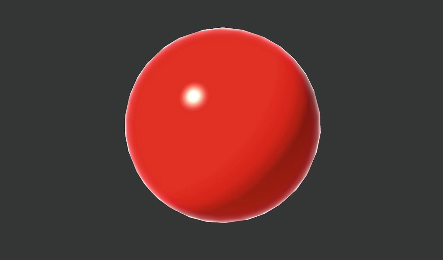
A vivid gradient sphere with a bright outline on a dark background. The colors get lighter on the top left of the sphere.

Let’s see how Phong shading can be implemented in HLSL and then in Shader Graph.

Phong Shading in HLSL

We’ll start by creating a new shader and naming it “PhongShading.shader”. The following code snippet is the skeleton shader we will develop in this section.

Shader "Examples/PhongShading"

{

      Properties

      {

            _BaseColor ("Base Color", Color) = (1, 1, 1, 1)

            _BaseTex("Base Texture", 2D) = "white" {}

            _GlossPower("Gloss Power", Float) = 400

      }

      SubShader

      {

            Tags

            {

                  "RenderType" = "Opaque"

                  "Queue" = "Geometry"

            }

            Pass

            {

                  Tags { ... }

                  HLSLPROGRAM

                  #pragma vertex vert

                  #pragma fragment frag

                  struct appdata

                  {

                        float4 positionOS : POSITION;

                        float2 uv : TEXCOORD0;

                        float3 normalOS : NORMAL;

                  };

                  struct v2f { ... }

                  v2f vert(appdata v) { ... }

                  float4 frag(v2f i) : SV_Target { ... }

                  ENDHLSL

            }

      }

}

Listing 10-38

Skeleton code for the PhongShading shader

You’ll need to make a few changes based on which render pipeline you are using. In the built-in pipeline, you’ll need to incorporate the following:

• Declare the properties inside HLSLPROGRAM by following Listing 10-25.

• Specify the correct tags by following Listing 10-8.

• Add the correct include files by following Listing 10-9.

And in URP, you’ll need to do the following:

• Declare the properties inside HLSLPROGRAM by following Listing 10-26.

• Specify the correct tags by following Listings 10-15 and 10-16.

• Add the correct include files by following Listing 10-17.

Now let’s explore how Phong shading differs from Gouraud shading. Most of the calculations will be moved from the vertex shader to the fragment shader, and the purpose of the vertex shader will be only to calculate the clip-space position, UVs, normal vector, and view vector required by the fragment shader. With that in mind, we no longer need to include lighting values inside the v2f struct, but we do need to include the normal vector and the view vector. We’ll use TEXCOORD1 and TEXCOORD2 for those.

struct v2f

{

      float4 positionCS : SV_POSITION;

      float2 uv : TEXCOORD0;

      float3 normalWS : TEXCOORD1;

      float3 viewWS : TEXCOORD2;

};

Listing 10-39

Modifying the v2f struct to include the normal vector and view vector

The code looks very different between the built-in pipeline and URP from here on, so I’ll split this section in two according to the render pipeline you’re using.

Phong Shading in the Built-In Pipeline

In the vertex shader, we must calculate the clip-space position and UVs like usual. Then we must calculate the normal vector and view vector to include them in the v2f struct. We can use the same UnityObjectToWorldNormal and WorldSpaceViewDir functions we previously used in the GouraudShading example. This time, we won’t need to normalize the view vector in the vertex shader for reasons we’re about to see.

v2f vert (appdata v)

{

      v2f o;

      o.positionCS = UnityObjectToClipPos(v.positionOS);

      o.uv = TRANSFORM_TEX(v.uv, _BaseTex);

      o.normalWS = UnityObjectToWorldNormal(v.normalOS);

      o.viewWS = WorldSpaceViewDir(v.positionOS);

      return o;

}

Listing 10-40

The vertex shader for Phong shading in the built-in pipeline

The lighting calculations we had previously performed inside the vertex shader are nowhere to be seen. Instead, what’s happening here is the normal and view vectors are being interpolated between each vertex so that we get per-fragment versions of those vectors. The snag here is that the interpolation step doesn’t renormalize those vectors, so they can have a length less than one, which will mess up our lighting calculations. Therefore, the first thing we’ll do in the fragment shader is renormalize them manually.

float4 frag (v2f i) : SV_TARGET

{

      float3 normal = normalize(i.normalWS);

      float3 view = normalize(i.viewWS);

Listing 10-41

Renormalizing the normal and view vectors

Once we’ve done that, the lighting code is largely a copy-and-paste job from the code we used in the vertex shader for Gouraud shading, except now the normal and view vectors don’t come from the v2f struct.

float3 normal = normalize(i.normalWS);

float3 view = normalize(i.viewWS);

float3 ambient = ShadeSH9(half4(i.normalWS, 1));

float3 diffuse = _LightColor0 * max(0, dot(normal, _WorldSpaceLightPos0.xyz));

float3 halfVector = normalize(_WorldSpaceLightPos0 + view);

float specular = max(0, dot(normal, halfVector));

specular = pow(specular, _GlossPower);

float3 specularColor = _LightColor0 * specular;

float4 diffuseLighting = float4(ambient + diffuse, 1.0f);

float4 specularLighting = float4(specularColor, 1.0f);

float4 textureSample = tex2D(_BaseTex, i.uv);

return textureSample * _BaseColor * diffuseLighting + specularLighting;

Listing 10-42

Calculating lighting in the fragment shader in the built-in pipeline

Once you’ve moved the lighting code to the fragment shader like this, you’ll instantly notice a better specular highlight on objects, as seen in Figure 10-23. The diffuse lighting calculations are also more accurate, but generally they’re not as noticeable as the specular highlight improvement. Let’s see how this works in URP.

Phong Shading in URP

We’ll start in the vertex shader by sending the clip-space position, UVs, normal vector, and view vector like we just did in the built-in pipeline example. We can use the TransformObjectToWorldNormal and GetWorldSpaceNormalizeViewDir functions like before, although we’ll be renormalizing the view vector in the fragment shader anyway, so let’s just use GetWorldSpaceViewDir instead.

v2f vert (appdata v)

{

      v2f o;

      o.positionCS = TransformObjectToHClip(v.positionOS.xyz);

      o.uv = TRANSFORM_TEX(v.uv, _BaseTex);

      o.normalWS = TransformObjectToWorldNormal(v.normalOS);

      float3 positionWS = mul(unity_ObjectToWorld, v.positionOS.xyz);

      o.viewWS = GetWorldSpaceViewDir(positionWS);

      return o;

}

Listing 10-43

The vertex shader for Phong shading in URP

Like with the built-in pipeline version of this shader, the problem with the normal and view vectors now is that they are not normalized due to the interpolation step, so the first thing we must do in the fragment shader is renormalize them with the normalize function as seen in Listing 10-41. Once that’s done, we can carry out the lighting calculations in the fragment shader using slightly different variable names and round off the shader by adding together the lighting contributions like we did in both the FlatShading and GouraudShading examples. One key difference is that instead of the SampleSHVertex function, which we used to calculate the ambient light in the previous examples, we’ll use SampleSH instead because it’s running in the fragment shader this time.

float4 frag (v2f i) : SV_Target

{

      float3 normal = normalize(i.normalWS);

      float3 view = normalize(i.viewWS);

      float3 ambient = SampleSH(i.normalWS);

      Light mainLight = GetMainLight();

      float3 diffuse = mainLight.color * max(0, dot(normal, mainLight.direction));

      float3 halfVector = normalize(mainLight.direction + view);

      float specular = max(0, dot(normal, halfVector));

      specular = pow(specular, _GlossPower);

      float3 specularColor = mainLight.color * specular;

      float4 diffuseLighting = float4(ambient + diffuse, 1.0f);

      float4 specularLighting = float4(specularColor, 1.0f);

      float4 textureSample = tex2D(_BaseTex, i.uv);

      return textureSample * _BaseColor * diffuseLighting + float4(specularColor, 1.0f);

}

Listing 10-44

Calculating lighting in the fragment shader in URP

The URP version of the shader now works the same as the built-in pipeline version as seen in Figure 10-23, and you should see a huge improvement in the specular highlight on objects with this shader. We can add Fresnel light to the equation with small additions to the shader.

Fresnel Light Modification

Adding Fresnel light to the PhongShading shader requires only a few lines of code. Fresnel light is inversely proportional to the dot product between the view vector and the normal vector, which we already have access to in the fragment shader. It’s also usually raised to a power of our choosing, so we can include that as a property. That’ll be the first addition we make to the shader.

Properties

{

      _BaseColor ("Base Color", Color) = (1, 1, 1, 1)

      _BaseTex("Base Texture", 2D) = "white" {}

      _GlossPower("Gloss Power", Float) = 400

      _FresnelPower("Fresnel Power", Float) = 5

}

Listing 10-45

Adding a _FresnelPower property to the Properties block

Typically, the powers used for Fresnel lighting are far lower than those used for specular highlights. We also need to declare the _FresnelPower property inside the HLSLPROGRAM block alongside the existing properties. The built-in pipeline and URP property declarations look slightly different, so pick the one for your pipeline.

float4 _BaseColor;

sampler2D _BaseTex;

float4 _BaseTex_ST;

float _GlossPower;

float _FresnelPower;

Listing 10-46

Declaring _FresnelPower in the built-in pipeline

CBUFFER_START(UnityPerMaterial)

      float4 _BaseColor;

      float4 _BaseTex_ST;

      float _GlossPower;

      float _FresnelPower;

CBUFFER_END

Listing 10-47

Declaring _FresnelPower in URP

There are no changes that need making to the structs or the vertex shader, so let’s jump straight to the fragment shader. The Fresnel calculation can slot in after the existing specular lighting calculation and just above the part where we add the lighting components together. The only difference between the code for the two pipelines is the variable used for the main light color.

float fresnel = 1.0f - max(0, dot(normal, view));

fresnel = pow(fresnel, _FresnelPower);

float3 fresnelColor = _LightColor0 * fresnel;

float4 diffuseLighting = float4(ambient + diffuse, 1.0f);

float4 specularLighting = float4(specularColor + fresnelColor, 1.0f);

Listing 10-48

Adding Fresnel lighting support in the built-in pipeline

float fresnel = 1.0f - max(0, dot(normal, view));

fresnel = pow(fresnel, _FresnelPower);

float3 fresnelColor = mainLight.color * fresnel;

float4 diffuseLighting = float4(ambient + diffuse, 1.0f);

float4 specularLighting = float4(specularColor + fresnelColor, 1.0f);

Listing 10-49

Adding Fresnel lighting support in URP

Once these lines of code are added, our objects will look like those in Figure 10-24. To round off this section, let’s see how Phong shading works in Shader Graph, complete with Fresnel lighting support at the end.

Phong Shading in Shader Graph

Phong shading in Shader Graph looks a lot like Gouraud shading in Shader Graph, except the calculations can now be done in the fragment stage rather than the vertex stage. We’ll also be adding Fresnel lighting support to the graph.

Start by creating a new Unlit graph and naming it “PhongShading.shadergraph”. We want to make sure Unity doesn’t automatically apply a second layer of lighting, so we can’t use a Lit graph. We can quickly get up to speed by using the Sub Graphs we created for the GouraudShading effect, as well as the nodes we used on the GouraudShading graph itself. The main difference is that we will not be adding either of the custom interpolators that we used for the GouraudShading graph. Follow these steps to get yourself up to speed:

• Add the same properties as seen in Figure 10-19.

• Add the set of nodes seen in Figure 10-20 for the diffuse light and ambient light calculations. Do not connect those nodes to a custom interpolator.

• Add the set of nodes seen in Figure 10-21 for the specular light calculations. Do not connect those nodes to a custom interpolator either.

• Add the nodes seen in Figure 10-22 for the final lighting calculations, except

  • Replace the DiffuseLighting custom interpolator node with the output of the diffuse light node group.

  • Replace the SpecularLighting custom interpolator node with the output of the specular light node group.

• Output the result of the final addition to Base Color on the master stack.

At this stage we have achieved Phong shading in Shader Graph, but let’s go one stage further and add Fresnel lighting support. First, we’ll need to add a Fresnel Power property as shown in Figure 10-25.

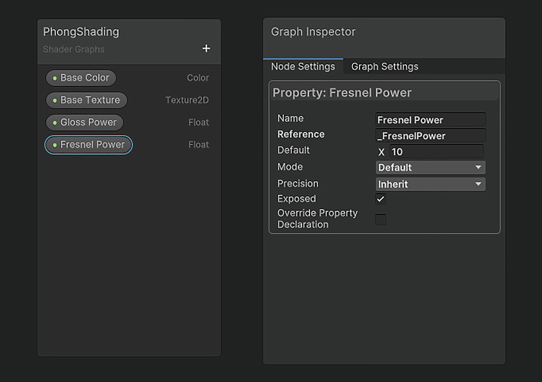
A graph inspector window lists properties of Fresnel power under the node settings tab with a Phong shading shader graph on the left. Fresnel power is highlighted.

Shader Graph has a Fresnel Effect node that automatically calculates Fresnel lighting for us. Better still, the default vectors that are input to the node are exactly the ones we need, and it has a Power input so that we don’t need to manually add a Power node after the Fresnel Effect node. Let’s add one to the graph, connect the Fresnel Power property, and add it to the existing diffuse and specular lighting components before outputting the result to the Base Color output on the master stack. Figure 10-26 shows how these nodes should be connected.

A dark screen illustrates how parameters of Fresnel lighting are added to the output to get the desired base color on the shading graph.

Now we have covered lighting objects in shaders by simulating the amount of ambient, diffuse, specular, and Fresnel lighting acting on the object. Next, we will see what functionality Unity provides out of the box to help us light objects without needing to calculate all the lighting ourselves.

Smoothness

Diffuse and specular light arise due to the way light reflects off a surface. Diffuse light occurs because incoming light rays get reflected in all directions due to complex interactions between the light and the surface of the object. A perfectly diffuse surface, one that reflects light equally in all directions, is called Lambertian; in fact, we have been using Lambertian reflectance as our model for diffuse light reflection in the shaders we have written. Although real-world materials don’t reflect light equally in all directions, Lambertian reflection is still a good approximation for diffuse reflection.

Specular lighting, on the other hand, arises when light rays reflect off a flat surface, which means most of the outgoing rays point in the same direction. Incoming light rays are reflected in the normal vector of the surface, so if a viewer is positioned at the correct angle, it will receive those reflected rays, resulting in a specular highlight on the object’s surface. Therefore, rough surfaces display almost no specular behavior, because the light rays are scattered rather than concentrated in a single direction. Mirrors are a special case of specular reflection, where almost all the light is reflected off the surface and almost none of it exhibits diffuse behavior. This is why shiny objects sometimes appear mirror-like. Figure 10-27 shows light rays reflecting off of a very smooth surface.

An illustration represents how light reflects while falling on a smooth surface in the same direction and scatters in different directions on the rough surface.

We can influence the amount of diffuse and specular light by modifying the smoothness of the surface. Objects with full smoothness will look very shiny – in other words, they have a high degree of specular reflection – and objects with low smoothness will primarily use the diffuse lighting component with little to no specular lighting. Very smooth objects may also appear mirror-like, as they reflect a large proportion of the environmental light, as seen in Figure 10-28.

A pair of vivid gradient spheres on a dark background. The left sphere is smoothened and outlined bright and the right has a matte surface.

Smoothness is only one part of PBR lighting. Typically, PBR shaders include two modes, which provide extra control over how an object is rendered: metallic mode, which lets us model objects on a scale between fully metallic and non-metallic, and specular mode, which gives us direct control over the color of specular reflections, rather than leaving it to other physical properties of the object. Let’s see how both modes work.

Metallic Mode

In metallic mode, we model the reflections of an object based on how much it acts like a metal. Fully non-metallic objects consist of a diffuse surface, with specular highlights visible on some parts of the object based on its smoothness. Fully metallic objects do not have a diffuse surface – the color of the object is based entirely on environmental reflections, although specular highlights still appear. A material in metallic mode will display specular reflections with a color that is based on the albedo of the object and the color of the incoming light. Figure 10-29 shows multiple objects with different levels of metallicity.

A quintet of vivid gradient spheres with bright outlines on a dark background. The color gets darker on the top surface of the sphere as we move towards the right, indicating metallicity.

Metallic mode is only one of two workflows commonly used with PBR. Specular mode may provide benefits if you want direct control over the specular highlight.

Specular Mode

In specular mode, we have more control over the color of specular highlights than in metallic mode. Whereas in metallic mode, the color of specular reflections is a result of the albedo color of the object and the color of the light, with specular mode, we can tint the specular highlights a specific color. A material in specular mode with high smoothness and high specularity will still appear mirror-like, as does a material in metallic mode with high smoothness and high metallicity. However, a high-specularity material typically loses its albedo color, unlike high-metallicity materials. If you want to design a metal object in specular mode, you need to tint the specular color and keep the albedo color black. Figure 10-30 shows multiple objects with different specular colors.

A quintet of vivid gradient spheres on a dark background. The color gets lighter as we move toward the right indicating the specular colors.

So far, we’ve seen that some components of our lighting models rely on the normal vector of the object’s surface. The next feature we’ll look at that is commonly featured in PBR shaders will let us modify the normal vector to simulate different surface shapes.

Normal Mapping

Normal mapping is a technique that lets us simulate detailed surfaces on an otherwise low-detail mesh using a texture (called a normal map). This allows us to add imperfections and other surface elements without needing to vastly increase the polygon count of the mesh. The advantage is that small details, which would otherwise require hundreds or even thousands of additional triangles to represent, can now be replaced by a texture that takes up comparatively little graphics memory, and we can use the same low-poly model with different normal maps if we want to swap out the surface details on an object easily.

Normal mapping works by modulating the normal vector at each point on the surface of an object. By doing so, lighting calculations produce a slightly different result, which makes the surface appear as if certain details existed, even if they are not physically present in the mesh. Figure 10-31 shows multiple versions of the same object with the same normal map, but different strengths.

A quintet of vivid gradient spheres on a dark background. The surface gets rough and resembles a plywood texture, as we move toward the right indicating increasing strength.

Although normal maps are not exclusive to PBR materials, they are certainly related to lighting, and they are used to mimic the physical properties of the surface, so I think it’s useful to introduce them alongside PBR materials. That said, you could create a shader that uses normal mapping with Blinn-Phong lighting if you wanted to. Normal maps have an indirect influence on the way lighting gets applied to an object. There is another kind of texture we can use to directly control the strength of ambient light on the object.

Ambient Occlusion

Some parts of a mesh receive less ambient light than others. For example, small cracks on the surface or folds and corners naturally have less light falling on them due to their shape. Furthermore, some parts of objects will always be obscured by other objects, such as the inner layers of clothing, resulting in less light reaching them. Ambient occlusion is a term that refers to when ambient light is prevented from reaching parts of an object – in other words, the light is occluded by another object. We can provide a grayscale occlusion map to represent the amount of occlusion on each part of a surface, where a value of 1 represents areas that should receive full ambient lighting and 0 means an area should receive no ambient light at all. Figure 10-32 shows two objects with and without occlusion.

A pair of vivid gradient spheres on a dark background. The left sphere has more plywood-like texture on the bottom when compared to the right sphere.

Now that we have seen a few textures that control the way external lights interact with the surface of the object, let’s see how objects can directly control light emission from their own surface.

Emission

Some objects emit light of their own, such as screens or neon lights. These objects continue to appear bright even if placed in a dark area, although non-emissive parts of the same object can still be influenced by lighting and shadows. We can model this in a PBR shader using emission to represent which areas of the object should emit light of a particular color. This comes in two parts: we can apply an emission map, which represents the emissive parts of the object through texturing, and an emissive color, which uses HDR colors that can go beyond the standard 0–255 range of color values if we want to represent a very bright surface. If you don’t apply an emission map, then the emission color will be applied to the entire object. Figure 10-33 shows multiple objects with increasing emissive strength.

A quintet of vivid gradient spheres on a dark background. The sphere radiates more light and gets brighter as we move toward the right.

You should now know about the most common components of a PBR shader and how they work in theory. Using this knowledge, let’s create a PBR shader in Unity for each pipeline in shader code and Shader Graph.

PBR in the Built-In Pipeline

In the built-in pipeline, we can use Unity’s surface shaders to help us with the lighting. Surface shaders are a feature that are exclusive to the built-in pipeline that let us define a lighting model (or use one included with Unity) and then define the surface properties of the object (such as albedo color, smoothness, emission, and the other properties listed previously). Then Unity will automatically carry out the lighting calculations for us. Let’s see how they work.

There’s a lot of unfamiliar code in this snippet, so let’s break down what’s happening. The first key difference is that the shader code is encased in a CGPROGRAM block rather than an HLSLPROGRAM block. Typically, modern Unity shaders are written in HLSL entirely, but surface shaders were designed in a time where Cg was the primary shading language in Unity, and as such, many of the built-in surface shader features are designed around that. Some of the built-in structs use the fixed data type, which doesn’t exist in HLSL. The fixed data type has at least 10 bits of fractional precision, although some hardware uses up to 32 bits, the same as a float. Otherwise, most shader syntax we’ve seen so far will work the same as in HLSL. Also, the code block is placed directly inside a SubShader rather than inside a Pass, because Unity may generate several shader passes based on the surface shader code.

In the preceding example, the Standard lighting model was used, which means the object will automatically have PBR lighting applied to the object. After specifying the lighting model, we can optionally add other shader features. In this example, the fullforwardshadows option means that Unity will generate shadows for multiple lights (we will focus on shadows later in this chapter).

UVs work slightly differently from regular shaders – to include them in Input, we must specify a float2 with the name of a texture prefixed with “uv”. For example, to include UVs that are set up to use the tiling and offset settings of the _BaseTex texture, we must include an entry in the Input struct called uv_BaseTex, which you can see in the preceding code snippet. In fact, we are going to include only this variable inside the Input struct.

Now, whenever we toggle the Boolean value of the _EmissionOn property on the material, Unity will turn the USE_EMISSION_ON keyword on or off according to the property’s value. We can use that to control whether emission is used in the shader. Speaking of which, we can now turn our attention to the surf function.

The surface shader is now complete, so you will now be able to attach it to a material and see PBR shading on your object. Try changing the material settings to see how different surface properties influence the appearance of the object. Now let’s see how PBR works in URP.

PBR in URP

As with the SurfaceData struct, we don’t need to populate every member of this struct, but it should give you a good idea of the features that you could add to the shader if you want. I’ve included a createInputData function to populate the struct. It takes a v2f as a parameter along with the tangent-space normal vector from SurfaceData. The most intensive part of this function is calculating the tangentToWorld matrix, which requires calculating the bitangent vector. Recall that the bitangent vector is perpendicular to both the normal and tangent vectors, and we can calculate it by taking the cross product of those two existing vectors.

With that, the PBR shader for URP is now complete, and you will see PBR lighting on any objects whose material uses this shader. As with the built-in pipeline version, try changing the properties of the material to see how the appearance of each object changes. Now that we have covered the PBR shader in shader code, let’s move on to Shader Graph.

PBR in Shader Graph

Shader Graph is by far the easiest tool to use for custom PBR shaders because both URP and HDRP ship with a preset Lit option that uses PBR calculations under the hood for lighting. Most of the work to be done inside a PBR shader for Shader Graph is setting up the properties and wiring up a few basic nodes to read them. Let’s create a new Lit shader and name it “PBR.shadergraph”. When you open it in the Shader Graph editor, you will be met with the following blocks on the master stack as shown in Figure 10-34.

A dark screen represents the properties of a Lit graph with vertex and fragment parameters. It has base color, normal tangent, metallic, smoothness, emission, and ambient occlusion.

You’ll see that several of the blocks are based on concepts we have discussed in this chapter so far, such as Normal, Metallic, Smoothness, Emission, and Ambient Occlusion. By default, a material uses metallic mode, so if you want to switch to specular mode, go to the Graph Settings and change the Workflow Mode option from Metallic to Specular. The Metallic block will automatically swap out for a Specular Color block. I’ll be using metallic mode. For this shader, we’ll be adding a lot of properties and then connecting them to the master stack outputs one by one. We’ll add the same properties to this graph that we added to the code versions of the shader, as seen in Figure 10-35.

A dark screen illustrates shader graph parameters of P B R. It has base color and texture, metallic map and strength, smoothness, normal map and strength, emission map and color.

Once these properties have all been added, we can sample each set of nodes and output them to the corresponding output on the master stack. Let’s deal with each output in order, starting with the Base Color output. For this, we can sample the Base Texture property and multiply the result by the Base Color property as shown in Figure 10-36.

A dark screen illustrates how the base color and the parameters of sample texture 2 D are multiplied to get the desired outcome and are fragmented into the base color.

Next is the Metallic output, which follows much the same process: sample the Metallic Map and multiply the result by Metallic Strength. Figure 10-37 shows how these nodes should be connected.

A dark screen of the metallic map illustrates how sample texture 2 D and metallic strength are multiplied to get the desired outcome and are fragmented into the base color.

After this, we can link up the Smoothness property to the Smoothness output, as shown in Figure 10-38. This is the simplest output since we just need to link the Smoothness property with the Smoothness block on the master stack.

A dark screen illustrates how smoothness property is mapped to fragments nodes of the shader graph that has base color, metallic, smoothness, normal, emission, and ambient occlusion.

Next is the Normal output block. For this, we will sample the Normal Map texture using a Sample Texture 2D node. By changing the Type to Normal at the bottom of the node, Unity will output normal vectors rather than color values from the texture. After this, we can apply the Normal Strength property to these vectors using a Normal Strength node, which takes the input vector and makes it longer or shorter according to the Strength value used as an input. Figure 10-39 shows how this node should be connected to other nodes.

A dark screen illustrates how normal strength modifies the parameters of sample texture 2 D with the normal strength and is mapped to the desired normal tangent space.

The penultimate output is the Emission, which requires slightly more work. To calculate the amount of emission, we can sample the Emission Map and multiply the output by Emission Color, like how we handled the Base Color output. However, we have also set up a property to turn emission on or off at will, so we’ll need to incorporate that. Drag the Use Emission keyword property onto the graph and connect the existing emission nodes into the On slot so that those values are used when emission is turned on. In the Off slot, use a value of 0, corresponding to black, which means there is no emission. Connect the output of this keyword node to the Emission block on the master stack. Figure 10-40 shows how these nodes should be connected.

A dark screen illustrates how the emission color and the parameters of sample texture 2 D are multiplied to get the desired outcome and are mapped into the fragments of emission.

The final output is the Ambient Occlusion, which is just a simple texture sample of Ambient Occlusion Map. Figure 10-41 shows how to connect these nodes to the output.

A dark screen illustrates how an ambient occlusion map is sampled along with its texture and U V 2 and is mapped into the fragments node of a graph.

Now that all these properties have been connected, you will see PBR lighting on objects. As with the code versions of this shader effect, try tweaking the material properties to see how the appearance of the object changes.

Thankfully, each of these PBR shaders applies shadows from other objects when calculating the amount of lighting on the object. However, some shaders are not yet able to cast shadows. In the next section, we’ll see how to add shadow-casting support to our shaders.

Shadow Casting in the Built-In Pipeline

Once you’ve added this pass to your shader, your objects should start to cast shadows, as seen in Figure 10-42. Now let’s see how the process of adding real-time shadows differs in URP.

Shadow Casting in URP

Once the shadow caster pass has been added to your shader, you will see shadows like those in Figure 10-42.

Shadow Casting in Shader Graph

In Shader Graph versions 11 and prior (for Unity 2021.1 and older), Lit and Unlit shaders automatically cast shadows. From our perspective, that’s great because we have to put in no extra work to get shadows working. To turn off shadows, you must disable them on a per-object basis by selecting the object and setting Cast Shadows to Off in the Lighting section of its Mesh Renderer as seen in Figure 10-43.

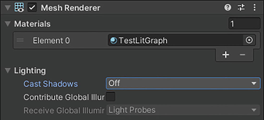
A mesh renderer dialog box lists materials of element 0 as Test Lit Graph and its lightings, where the cast shadows are turned off.

In Shader Graph 12.0 and up (for Unity 2021.2 and later), you can turn off shadow casting on a per-shader basis instead. In the Graph Settings of a Lit or Unlit shader, go to the Cast Shadows option and untick the box to prevent Unity from generating the shadow caster pass, as shown in Figure 10-44.

A graph inspector window lists options under graph settings that have precision, target, and universal settings, where cast shadow is selected.

It’s as easy as that – just untick a box! With that, you should know how to enable and disable shadow casting in each of Unity’s pipelines and in Shader Graph.