© The Author(s), under exclusive license to APress Media, LLC, part of Springer Nature 2022
D. IlettBuilding Quality Shaders for Unity®https://doi.org/10.1007/978-1-4842-8652-4_12

12. Advanced Shaders

Daniel Ilett1  
(1)
Coventry, UK
 

So far, we have primarily discussed vertex and fragment shaders that take meshes, transform their vertices onto the screen, and color the pixels. Most shaders take this form. We’ve already seen the power of these types of shaders and the broad range of capabilities they have, but they are not the only types of shaders. In the shader pipeline, there are two optional stages that we have not yet encountered: the tessellation shader and the geometry shader. On top of that, there are compute shaders, which operate outside the usual mesh shading pipeline and can be used for arbitrary calculations on the GPU. In this chapter, we will explore some of these strange and exotic new types of shaders and add ever-powerful new tools to our box of tricks.

Tessellation Shaders

Back all the way in Chapter 1, I presented a simplified diagram of the shader pipeline with six “stages,” although in that diagram I lumped together tessellation and geometry shaders together into one box as “optional” stages to avoid complicating things (see Figure 1-1). Let’s revisit and flesh out that diagram now in Figure 12-1 with a different example and split tessellation and geometry shaders into stages 3a and 3b. Then, let’s discuss in detail what the tessellation stage is doing.

A rendering graphics pipeline converts the raw vertex data to per fragment operations through the vertex, tessellation and geometry shader, rasterization, and fragment shader.

Figure 12-1

The shader pipeline stages. In this example, a quad mesh is turned into a grassy mesh with blades – new geometry – growing out of new vertices created during the pipeline

So what is changing between stage 2, the vertex shader, and stage 3a, the tessellation shader? Recall that the vertex shader just moves vertices around – it has no power at all to create or destroy vertices, and each vertex only knows about itself. On the other hand, here’s what the tessellation shader does:
  • The tessellation shader can create new vertices by subdividing an existing face of a mesh.

  • The tessellation shader can create new vertices on the edges or within the face of each triangle of a mesh.

  • Calling it a “tessellation shader” is slightly misleading because there are actually two programmable stages and one fixed-function stage involved in the process:
    • The tessellation control shader (TCS), also called the hull shader, defines how much tessellation should be applied to each face. This shader is not required for tessellation, although we will be including it in each example.

    • It receives a patch made up of a small handful of vertices, and it can use information about those vertices to control the amount of tessellation. Unlike vertex shaders, hull shaders can access data about multiple vertices at once. We can configure the number of vertices in each patch.

    • The tessellation primitive generation fixed-function stage, also called the “tessellator,” is situated between the two programmable stages. It creates new primitives (i.e., triangles or quads) based on the hull shader output.

    • The tessellation evaluation shader (TES), also called the domain shader, is responsible for positioning the vertices output by the tessellator.

    • Although the domain shader is typically used to interpolate the position of new vertices based on the positions of existing vertices, you may change the position however you want. It is commonly used to offset the positions of vertices.

If some of this went over your head on the first read-through, don’t worry – it clicked for me a lot more the first time after I worked through an example. There are many cases where tessellation can be used to achieve more aesthetically pleasing results, so let’s start with a water wave effect.

Tip

Tessellation is often seen as a more advanced shader feature – after all, it’s completely optional, and there are many moving parts to it. I’ve put it in the “Advanced Shaders” chapter for that reason. But keep in mind that, like any other shader, it’s just made up of relatively small functions! Take the code I’ve written and try adding, removing, and hacking bits of it around to see what changes on-screen – hands-on experience will likely help you deepen your understanding of tessellation.

Water Wave Effect with Tessellation

Water is a common feature in games, and many of those games use a shader to apply waves that bob up and down to the water surface. These effects work by moving the vertices of the mesh up and down in world space over time to simulate waves rolling over the surface, and for this effect, we will do just that. Although this shader could be applied to any mesh, it will work best if applied to any flat plane mesh – Unity’s built-in quad will do just fine. However, if we just displace the vertices, the effect will obviously look worse on a low-poly mesh than a high-poly one. That’s where tessellation shaders come in. It would probably be wasteful to create a high-poly mesh in the Assets folder just for higher-quality water, so instead, we can take a basic quad and subdivide it with tessellation at runtime to end up with a high-poly mesh. That way, the waves will appear smoother, as seen in Figure 12-2.

A pair of screens represent the triangular sheet of a wave mesh shaded lightly without tessellation, and the subdivision of each wave quad results in a smoother wave mesh.

Figure 12-2

Two instances of Unity’s built-in plane mesh with a wave effect applied and different tessellation settings used. On the left, no tessellation is used. On the right, each quad is subdivided eight times, resulting in smoother waves

To visualize the wireframe of a mesh in the Scene View as in Figure 12-2, you can change the Shading Mode from Shaded to either Wireframe or Shaded Wireframe (see Figure 12-3). This option is on the toolbar just above the Scene View window.

A screenshot lists the menu under the shading mode, where the shaded wireframe is selected.

Figure 12-3

Changing the Shading Mode to Shaded Wireframe

We’ll start by creating the effect in shader code and then see how it works in Shader Graph.

Note

In Unity 2021.3 LTS, tessellation is only compatible with HDRP Shader Graph, so unfortunately, we won’t be able to use URP Shader Graph for this effect.

Wave Tessellation in Shader Code

Let’s start with a skeleton shader file containing all the structs and functions and then fill them in one at a time. I’ll explain each part of the shader in roughly the order they happen in the graphics pipeline. Create a new shader file called “Waves.shader” and replace its contents with the following code.
Shader "Examples/Waves"
{
      Properties
      {
            _BaseColor ("Base Color", Color) = (1, 1, 1, 1)
            _BaseTex("Base Texture", 2D) = "white" {}
             [Enum(UnityEngine.Rendering.BlendMode)]
            _SrcBlend("Source Blend Factor", Int) = 1
             [Enum(UnityEngine.Rendering.BlendMode)]
            _DstBlend("Destination Blend Factor", Int) = 1
      }
      SubShader
      {
            Tags
            {
                  "RenderType" = "Transparent"
                  "Queue" = "Transparent"
            }
            Pass
            {
                  Blend [_SrcBlend] [_DstBlend]
                  HLSLPROGRAM
                  struct appdata { ... };
                  struct tessControlPoint { ... };
                  struct tessFactors { ... };
                  struct v2f { ... };
                  sampler2D _BaseTex;
                  CBUFFER_START(UnityPerMaterial)
                        float4 _BaseColor;
                        float4 _BaseTex_ST;
                  CBUFFER_END
                  tessControlPoint vert( ... ) { ... }
                  v2f tessVert( ... ) { ... }
                  tessFactors patchConstantFunc( ... ) { ... }
                  tessControlPoint tessHull( ... ) { ... }
                  v2f tessDomain( ...) { ... }
                  float4 frag(v2f i) : SV_Target { ... }
                  ENDHLSL
            }
      }
      Fallback Off
}
Listing 12-1

The wave tessellation shader skeleton

This shader is set up to use transparent rendering, with _SrcBlend and _DstBlend properties to customize how transparency blending works. If you are using URP, then include the following tag inside the SubShader Tags block.
Tags
{
      "RenderType" = "Transparent"
      "Queue" = "Transparent"
      "RenderPipeline" = "UniversalPipeline"
}
Listing 12-2

URP RenderPipeline tag

Then also include a new Tags block inside the Pass, just under the Blend keyword.
Blend [_SrcBlend] [_DstBlend]
Tags
{
      "LightMode" = "UniversalForward"
}
Listing 12-3

URP forward pass tag

Finally, we’ll include required files. In the built-in pipeline, we need the UnityCG.cginc file, and in URP, we need the Core.hlsl file.
#include "UnityCG.cginc"
struct appdata { ... };
Listing 12-4

Required files for the built-in pipeline

#include "Packages/com.unity.render-pipelines.universal/ShaderLibrary/Core.hlsl"
struct appdata { ... };
Listing 12-5

Required files for URP

Next, let’s add the properties for this shader. We need two Float properties called _WaveStrength and _WaveSpeed to control the height of the waves and the speed they move across the mesh, respectively. We will also include a third Float property called _TessAmount to control how much tessellation happens across the mesh – a higher value means more vertices get added to each triangle. The minimum amount is 1, meaning no vertices are added, and the maximum is 64, which is the highest number of subdivisions the hardware supports.
Properties
{
      _BaseColor ("Base Color", Color) = (1, 1, 1, 1)
      _BaseTex("Base Texture", 2D) = "white" {}
      _WaveStrength("Wave Strength", Range(0, 2)) = 0.1
      _WaveSpeed("Wave Speed", Range(0, 10)) = 1
       [Enum(UnityEngine.Rendering.BlendMode)]
      _SrcBlend("Source Blend Factor", Int) = 1
       [Enum(UnityEngine.Rendering.BlendMode)]
      _DstBlend("Destination Blend Factor", Int) = 1
      _TessAmount("Tessellation Amount", Range(1, 64)) = 2
}
Listing 12-6

Wave shader properties

We’ll also need to add these properties in the HLSLPROGRAM block. The code looks slightly different between the built-in pipeline and URP.
struct v2f { ... };
sampler2D _BaseTex;
float4 _BaseColor;
float4 _BaseTex_ST;
float _TessAmount;
float _WaveStrength;
float _WaveSpeed;
Listing 12-7

Adding wave shader properties in the built-in pipeline

struct v2f { ... };
sampler2D _BaseTex;
CBUFFER_START(UnityPerMaterial)
      float4 _BaseColor;
      float4 _BaseTex_ST;
      float _TessAmount;
      float _WaveStrength;
      float _WaveSpeed;
CBUFFER_END
Listing 12-8

Adding wave shader properties in URP

Now we can move on to the HLSLPROGRAM block. As you can see in Listing 12-1, there are many structs and functions, some of which are familiar and others of which are brand-new. First, we’ll tell Unity which functions correspond to which shaders with #pragma statements. The #pragma hull <name> and #pragma domain <name> statements tell Unity which functions make up the hull and domain shaders – in our case, these functions are called tessHull and tessDomain, respectively. We also need to say #pragma target 4.6, since 4.6 is the earliest of Unity’s shader models that supports tessellation. It’s roughly equivalent to OpenGL version 4.1 and DirectX 11.
HLSLPROGRAM
#pragma vertex vert
#pragma fragment frag
#pragma hull tessHull
#pragma domain tessDomain
#pragma target 4.6
Listing 12-9

#pragma statements for tessellation

Now, you may have noticed something strange in Listing 12-1. Not only do we have the vert function but I’ve added an additional function named tessVert, which looks suspiciously like an extra vertex shader function. Here’s why. Ordinarily, the vertex shader is used to transform data about meshes from object space to clip space, but this shader will be different; I want to offset the vertices of the mesh upward in world space after the tessellation shader has run (indeed, the entire point of the shader is to smooth out the shape of those waves). However, the vertex shader always runs first. Therefore, I’m supplying two vertex functions: one called vert, which is “officially” the vertex shader for this file, and another called tessVert, which I will run manually after all tessellation has been applied.

Wave Vertex Shader
The vert function will act as a pass-through; all the parameters it is passed in appdata will be unchanged and passed on to v2f. First, let’s look at appdata. It’s going to be very basic – the only data required by the shader is the object position and associated UV data of each vertex. We’ve seen this many times before.
struct appdata
{
      float4 positionOS : Position;
      float2 uv : TEXCOORD0;
};
Listing 12-10

The appdata struct for the wave effect

Before we write the vertex shader, let’s think about what it will output. Usually, we would output a v2f struct containing clip-space positions and UVs, but as I mentioned, vert is going to output unchanged object-space positions and UVs. The next stage of the pipeline is the tessellation control shader, also called the hull shader. The hull shader expects to receive data about each control point (i.e., vertex) from the vertex shader. Therefore, I will create a struct called tessControlPoint to control what data gets passed between the vertex shader and the hull shader. The only difference is that the positionOS member of tessControlPoint uses the INTERNALTESSPOS semantic instead of POSITION. This struct is like any other, so you could add additional members if you wanted to do extra calculations in this vertex shader, such as generating normal vector information on the fly. However, I just want to use the vertex shader as a pass-through, so I will use the same members in tessControlPoint as in appdata.
struct tessControlPoint
{
      float4 positionOS : INTERNALTESSPOS;
      float2 uv : TEXCOORD0;
};
Listing 12-11

The tessControlPoint struct for the wave effect

Now let’s write the vert vertex function. Each member of appdata will be copied into the tessControlPoint struct.
tessControlPoint vert(appdata v)
{
      tessControlPoint o;
      o.positionOS = v.positionOS;
      o.uv = v.uv;
      return o;
}
Listing 12-12

The vert vertex function

That’s the vertex stage complete, and we can move on to the hull shader.

Wave Tessellation Control (Hull) Shader
The hull shader has two core responsibilities. First, it will output a list of control points that the tessellator uses as a base to perform subdivision on (in other words, we usually output the same geometric primitives that were input, like triangles). This can be done inside the body of the tessHull function. Second, it will output a set of tessellation factors that control how the inside portion and the edges of each primitive get subdivided. tessHull can’t return two sets of data, so we specify these factors in a separate function called a patch constant function. Both stages run in parallel. We have a high degree of control over the inputs and outputs of the hull shader using attributes that get placed above the tessHull function – let’s see how it all works:
  • The tessHull function takes in a patch of control points.

  • Think of a patch as a single polygon. It can be between 1 and 32 control points, but in our case, we’ll just use 3, which is a triangle.

  • The hull shader can access all control points in that patch.

  • The first parameter to the hull shader is the patch itself. We specify what data each vertex holds (in our case, each one is a tessControlPoint) and how many vertices are in the patch (3).

  • The second parameter is the ID of a vertex in the patch. The hull shader runs once per vertex and outputs one vertex per invocation.

  • The output of tessHull will just be one vertex. We’ll use the ID parameter to grab a vertex from the patch and then return that vertex.

  • To tell Unity we are using triangles, we’ll need a few attributes:
    • The domain attribute (not to be confused with the domain shader) takes the value tri. Other possible values are quad or isoline – these values depend on what type of mesh you have.

    • The outputcontrolpoints attribute is used to define how many control points are created per patch. We’ll use the value 3.

    • The outputtopology attribute is used to define what primitive types should be accepted by the tessellator. This is also based on the mesh used. In our case, we’ll use triangle_cw, which means triangles with clockwise winding order. Other possible values are triangle_ccw (i.e., counterclockwise winding order), point, and line.

[domain("tri")]
[outputcontrolpoints(3)]
[outputtopology("triangle_cw")]
tessControlPoint tessHull(InputPatch<tessControlPoint, 3> patch, uint id : SV_OutputControlPointID)
{
      return patch[id];
}
Listing 12-13

The tessHull function

We’re not done yet. We also need a partitioning attribute to define how the tessellator deals with the tessellation factors (we’ll deal with those factors soon). Each partition mode defines how new subdivisions get formed when you change the tessellation factor associated with the inside or an edge. Here are the possible values:
  • integer – Snap tessellation factors to the next highest integer value. All subdivisions are equally spaced.

  • fractional_even – When using non-integer factors, an extra subdivision will appear when going between one even-numbered factor and the next. This subdivision is not equally spaced with nearby subdivisions – it grows as the tessellation factor increases until you hit an even number.

  • fractional_odd – Same as fractional_even, but the changes apply to odd-numbered factors instead.

  • pow2 – This seems to be the same as integer in the cases I tried out.

The final attribute is the patchconstantfunc attribute, which we use to specify the patch constant function that I mentioned before. We input the function name, which in our case is just patchConstantFunc.
[domain("tri")]
[outputcontrolpoints(3)]
[outputtopology("triangle_cw")]
[partitioning("fractional_even")]
[patchconstantfunc("patchConstantFunc")]
tessControlPoint tessHull(InputPatch<tessControlPoint, 3> patch, uint id : SV_OutputControlPointID)
{
      return patch[id];
}
Listing 12-14

Partitioning and patch constant function attributes

With all the attributes in place, let’s move on to the patch constant function. As I mentioned, the purpose of this function is to generate a set of tessellation factors that will be used by the tessellator to generate brand-new control points. For triangles, there are four factors: three of them are attached to each edge of the triangle, and the last one is for the center of the triangle. For example, if I were to give an edge a factor of 2, then Unity would split the edge into two segments by generating one new vertex in the middle of the edge and replacing the original triangle with two smaller triangles as necessary. If I give the inside a factor of 2, Unity adds one new vertex in the center of the triangle. Figure 12-4 shows you what objects look like using different factors.

An illustration depicts the three shaded quadrilaterals of a unity quad, fragmented into one, two, and four quads with different tessellation factors.

Figure 12-4

Three versions of the default Unity quad with different tessellation factors. From left to right, the edges and the inside of the mesh use 1, 2, and 4 as their tessellation factors, respectively

First, we will set up a struct for these factors called tessFactors. The edge factors are contained inside a small array of floats with three entries, which uses the SV_TessFactor semantic. The inside factor is a single float value with the SV_InsideTessFactor semantic.
struct tessFactors
{
      float edge[3] : SV_TessFactor;
      float inside : SV_InsideTessFactor;
};
Listing 12-15

The tessFactors struct

Now let’s write the patchConstantFunc function. It takes in a patch and outputs a set of tessFactors for this patch. Although it’s possible to give each edge a different factor, we’ll give all three edges and the center the same factor, _TessAmount, to keep things simple.
tessFactors patchConstantFunc(InputPatch<tessControlPoint, 3> patch)
{
      tessFactors f;
      f.edge[0] = f.edge[1] = f.edge[2] = _TessAmount;
      f.inside = _TessAmount;
      return f;
}
Listing 12-16

The patch constant function

Now that we have handled both sides of the hull shader, we can move on to the domain shader.

Wave Tessellation Evaluation (Domain) Shader

The tessellator takes the control points output by the hull shader and the tessellation factors output by the patch constant function and calculates new control points, which it passes to the domain shader. The domain shader is invoked once per new control point; the parameters to the domain shader are the tessellation factors from the patch constant function, the patch output by the hull shader, and a set of coordinates. These are the barycentric coordinates of the new point, which denote how far the new vertex is from the original three control points on the triangle. For example, a vertex with barycentric coordinates (0.5, 0.5, 0) lies exactly on the halfway point of one of the triangle’s edges. These coordinates use the SV_DomainLocation semantic.

The responsibility of the domain shader is to interpolate the new vertex data between each of the original triangle’s vertices and return a v2f struct. Our domain shader uses the tessDomain function, so we will edit that. First, we’ll add a domain attribute to it to specify we are using triangles. Then, in the function body, we’ll create a new appdata struct and interpolate each of the members of the tessControlPoint between those barycentric coordinates and then put the results into appdata. Remember how this file has two vertex functions? We’ll pass the appdata into the tessVert function and return that. tessVert takes in an appdata and returns a v2f, like most of the vertex shaders we saw in previous chapters.
[domain("tri")]
v2f tessDomain(tessFactors factors, OutputPatch<tessControlPoint, 3> patch, float3 bcCoords : SV_DomainLocation)
{
      appdata i;
      i.positionOS = patch[0].positionOS * bcCoords.x +
            patch[1].positionOS * bcCoords.y +
            patch[2].positionOS * bcCoords.z;
      i.uv = patch[0].uv * bcCoords.x +
            patch[1].uv * bcCoords.y +
            patch[2].uv * bcCoords.z;
      return tessVert(i);
}
Listing 12-17

The tessDomain function

Remember that at this point, all the calculations have been operating in object space – it is still necessary to transform from object to clip space. That’s what the tessVert function will do.

Wave Tessellation tessVert Function and Fragment Shader
We are now solidly out of the land of tessellation shaders and back onto familiar ground, working with just vertices and fragments. The tessVert function takes in an appdata struct and outputs a v2f struct. Rather than just transforming between object and clip space, as do most of the vertex functions we have written throughout the book, here’s what this shader will do:
  • We will transform the vertices to world space with unity_ObjectToWorld, a matrix that is provided by Unity.

  • Then, we’ll apply a height offset based on the time since level start, the _WaveSpeed property value, and the x- and z-positions of the vertex in world space.
    • By applying a sine function to those variables, the waves will bob up and down over time.

  • We’ll then multiply the offset by _WaveStrength so that we have control over the physical size of the waves and add it to the y-position in world space.

  • We can then transform the position from world to clip space with UNITY_MATRIX_VP. We need the positions to be in clip space before rasterization, so we’re finished with positions now.

  • Finally, we’ll use TRANSFORM_TEX to deal with tiling and offsetting the UVs.

v2f tessVert(appdata v)
{
      v2f o;
      float4 positionWS = mul(unity_ObjectToWorld, v.positionOS);
      float height = sin(_Time.y * _WaveSpeed + positionWS.x + positionWS.z);
      positionWS.y += height * _WaveStrength;
      o.positionCS = mul(UNITY_MATRIX_VP, positionWS);
      o.uv = TRANSFORM_TEX(v.uv, _BaseTex);
      return o;
}
Listing 12-18

The tessVert function

The tessVert function is called inside the tessDomain function, which returns a v2f struct. Since we have no geometry shader, the next stage in the shader pipeline after the domain shader is the fragment shader, which receives the v2f struct as its input. The frag function is the simplest shader in this whole file – all it does is sample _BaseTex and multiply by _BaseColor.
float4 frag(v2f i) : SV_Target
{
      float4 textureSample = tex2D(_BaseTex, i.uv);
      return textureSample * _BaseColor;
}
Listing 12-19

The fragment shader

With that, you should be able to see tessellation on your objects using this shader, as in Figure 12-2. Obviously it’s difficult to showcase the quality of an animation in a book, so play around with the tessellation factors in the code to see how it impacts the smoothness of the waves on your own computer. You will probably be able to find a sweet spot where the waves start looking smooth, and increasing the tessellation factors past that point has diminishing returns. Now that we have created tessellated waves in shader code, let’s see how the same can be achieved with Shader Graph.

Wave Tessellation in Shader Graph

Tessellation became available in Shader Graph with HDRP version 12.0, corresponding to Unity 2021.2. Unfortunately, URP Shader Graph does not yet support tessellation, so this effect will only work in HDRP. On the flipside, tessellation is a lot easier to achieve with Shader Graph. Let’s see how.

I’ll start by creating an Unlit graph (you can use a Lit graph if you want – pick whichever looks best for your use case) and name it “Waves.shadergraph”. We’ll start by adding properties to the graph:
  • A Color named Base Color that will provide a way to tint the albedo of the water.

  • A Texture2D called Base Texture that will also affect the albedo.

  • A Float called Wave Speed that is used to control how fast the waves spread across the surface of the water.

  • A Float called Wave Strength that represents how high and low the waves travel in world space. A value of 1 means the waves travel one Unity unit up and down.

  • A Float called Tess Factor (short for “tessellation factor”) that we’ll use to configure how many times the mesh gets subdivided. This property should use a slider between 1 and 64 (1 means no subdivisions, and 64 is the hardware limit).

With these properties in place, let’s enable tessellation on the graph. Remember: this only works on HDRP in the latest LTS release of Unity as of the writing of this book (Unity 2021.3). Go to the Graph Settings tab of the Graph Inspector and expand the Surface Options section. Here, you will find settings such as opaque/transparent rendering (I’ll use transparent for this graph, but you can use either), alpha clipping, double-sided rendering, and so on. One of the options is labeled Tessellation, and by ticking it, a few more options appear, and two new blocks appear on the vertex stage of the master stack. Those new options are as follows:
  • Max Displacement – The maximum distance, in Unity units, that the tessellated triangles can be displaced from their original position. This isn’t a hard limit, but it prevents triangles being improperly culled.

  • Triangle Culling Epsilon – Higher values mean that more triangles are culled.

  • Start Fade Distance – At this distance (in Unity units) from the camera, tessellation will start to fade by reducing the tessellation factor.

  • End Fade Distance – At this distance (in Unity units) from the camera, tessellation stops (i.e., the tessellation factor is 1).

  • Triangle Size – When a triangle is above this size, in pixels, HDRP will subdivide it. Lower values mean smaller triangles get subdivided, and therefore the resulting mesh will be smoother.

  • Tessellation Mode – Choose between None and Phong. With Phong tessellation, Unity will interpolate the newly generated geometry to smooth the mesh.

I will set the Max Displacement to 1 and leave the other values with their defaults. The two new blocks on the vertex stage, which are of more interest to us, are
  • Tessellation Factor – This is the same as the tessellation factor we saw in the code-based tessellation shader. This is the number of times a triangle is subdivided. However, there is no way to provide different edge factors for each edge or inside factors for the inside of the triangle – they all use the same value.

  • Tessellation Displacement – This is the offset, in world space, of the vertices of the mesh. The offset is applied after tessellation, so it just happens to be perfect for the wave effect we’re building.

With these blocks accessible on the master stack, we can get to work creating the wave effect. First, connect the Tess Factor property to the Tessellation Factor block. This will let us dynamically change the amount of tessellation on each material that uses this shader.

Next, we’ll set up the output for the Tessellation Displacement block. As we did with the code-based wave shader, we’ll add time multiplied by the Wave Speed property to the x- and z-positions of the vertex in world space and then apply a sine function to the result. We’ll multiply that by the Wave Strength property and output it as a y-offset. When we’re accessing the vertex position with the Position node, be careful to change the Space to Absolute World instead of World, because the latter is relative to the camera position, which would cause the waves to move erratically when the camera moves! See Figure 12-5 to see how the nodes are set up.

A screenshot of the shader graph illustrates the calculation of the tessellation displacement through the parameters of wave speed and strength with the tess factor.

Figure 12-5

Tessellation Factor and Tessellation Displacement in Shader Graph

With these nodes in place, Unity will perform tessellation, add the tessellation offset to the vertices of the newly subdivided mesh, and then rasterize the mesh and apply the fragment stages to the pixels of the object. We’ll deal with the fragment stage now. We’ll use a node structure we’ve seen countless times before – sample the Base Texture with a Sample Texture 2D node, multiply the result by the Base Color property, output the result to the Base Color block, and then split off the alpha component and output it to the Alpha block on the master stack. See Figure 12-6 to see these nodes in action.

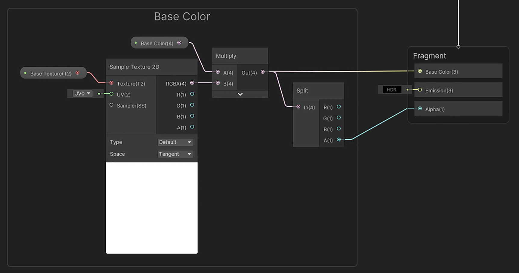
A screenshot of the base color window represents, how the properties of the base color are multiplied and split into output fragments.

Figure 12-6

Outputting the Base Color

The graph is now complete, and you should see results just like those we saw with the code-based version of the shader (see Figure 12-2). Note that as you change the tessellation factor property, Unity will use fractional_odd subdivision behavior when using non-integer values, rather than the “integer” behavior we used with the code-based shader.

As you can see, tessellation is a powerful technique that can achieve things that are impossible with the vertex and fragment shaders we have used throughout the book so far. In the next example of tessellation, we will build a simplified LOD system that uses a high tessellation factor for objects close to the screen and a low tessellation factor when objects are far from the screen.

Level of Detail Using Tessellation

For the wave shader, we used a uniform amount of tessellation for each object – that is, every triangle of each object using a material with this shader used the same tessellation factor. That doesn’t have to be the case. When a mesh is close to the camera, we want to use a high tessellation factor so that we get the most benefits out of the slightly increased processing time. But when a mesh is far away, we can get away with using a far lower tessellation factor. Even for large objects that exist both close to and far away from the camera, it is in our best interest to use lots of tessellations for the closest triangles and not as much for the furthest ones. In this shader example, we’ll forget about waves and see how we can build a tessellation-based LOD system for a basic stationary mesh. Let’s see how to do this in shader code and then in HDRP Shader Graph.

Level of Detail Tessellation in Shader Code

Let’s go over the structure of the file. This time, I’ll just use one vertex function at the start and do all the v2f processing in tessDomain. We’ll be using the same set of functions as the wave shader, but the flow of data between the stages will be slightly different in ways I’ll explain as we go. Start by creating a new shader file and naming it “TessLOD.shader”. Here’s the basic skeleton of the file.
Shader "Examples/TessLOD"
{
      Properties
      {
            _BaseColor ("Base Color", Color) = (1, 1, 1, 1)
            _BaseTex("Base Texture", 2D) = "white" {}
             [Enum(UnityEngine.Rendering.BlendMode)]
            _SrcBlend("Source Blend Factor", Int) = 1
             [Enum(UnityEngine.Rendering.BlendMode)]
            _DstBlend("Destination Blend Factor", Int) = 1
            _TessAmount("Tess. Amount", Range(1, 64)) = 2
      }
      SubShader
      {
            Tags
            {
                  "RenderType" = "Transparent"
                  "Queue" = "Transparent"
            }
            Pass
            {
                  Blend [_SrcBlend] [_DstBlend]
                  HLSLPROGRAM
                  #pragma vertex vert
                  #pragma fragment frag
                  #pragma hull tessHull
                  #pragma domain tessDomain
                  #pragma target 4.6
                  struct appdata
                  {
                        float4 positionOS : Position;
                        float2 uv : TEXCOORD0;
                  };
                  struct tessControlPoint { ... };
                  struct tessFactors
                  {
                        float edge[3] : SV_TessFactor;
                        float inside : SV_InsideTessFactor;
                  };
                  struct v2f
                  {
                        float4 positionCS : SV_Position;
                        float2 uv : TEXCOORD0;
                  };
                  tessControlPoint vert(appdata v) { ... }
                  tessFactors patchConstantFunc( ... ) { ... }
                  [domain("tri")]
                  [outputcontrolpoints(3)]
                  [outputtopology("triangle_cw")]
                  [partitioning("integer")]
                  [patchconstantfunc("patchConstantFunc")]
                  tessControlPoint tessHull(InputPatch<tessControlPoint, 3> patch, uint id : SV_OutputControlPointID)
                  {
                        return patch[id];
                  }
                  [domain("tri")]
                  v2f tessDomain( ... ) { ... }
                  float4 frag(v2f i) : SV_Target
                  {
                        float4 textureSample = tex2D(_BaseTex, i.uv);
                        return textureSample * _BaseColor;
                  }
                  ENDHLSL
            }
      }
      Fallback Off
}
Listing 12-20

The TessLOD shader skeleton

There are a few key similarities between this and the Waves shader. The tessHull and frag functions are identical, and most of the structs are the same. However, we’re going to make changes to the vert, patchConstantFunc, and tessDomain functions, as well as the tessControlPoint struct. I’ve also removed all mentions of the properties related to waves. There are also pipeline-specific changes that must be made:
  • If you’re working in the built-in pipeline, you’ll need to follow Listing 12-4 to add the correct include file.

  • In URP, instead follow Listing 12-5 for the relevant include file and then follow Listings 12-2 and 12-3 to add the correct tags to the shader.

With those small edits out of the way, let’s add properties for this shader. We will need two new Float properties called _TessMinDistance and _TessMaxDistance, which do the following:
  • When the distance of an edge (in Unity units) from the camera is less than _TessMinDistance, those edges use the full tessellation factor, defined in the _TessAmount property.

  • When the distance is above _TessMaxDistance, the mesh uses a tessellation factor of 1, which means there is no tessellation at all.

  • When the distance of an edge is between the two properties, the tessellation factor gets smaller the further from the camera you get.

With these properties, the Properties block looks like the following.
Properties
{
      _BaseColor ("Base Color", Color) = (1, 1, 1, 1)
      _BaseTex("Base Texture", 2D) = "white" {}
       [Enum(UnityEngine.Rendering.BlendMode)]
      _SrcBlend("Source Blend Factor", Int) = 1
       [Enum(UnityEngine.Rendering.BlendMode)]
      _DstBlend("Destination Blend Factor", Int) = 1
      _TessAmount("Tessellation Amount", Range(1, 64)) = 2
      _TessMinDistance("Min Tessellation Distance", Float) = 20
      _TessMaxDistance("Max Tessellation Distance", Float) = 50
}
Listing 12-21

The Properties block

We’ll need to define them inside the HLSLPROGRAM block too. The code is slightly different between the built-in pipeline and URP.
struct v2f { ... };
sampler2D _BaseTex;
float4 _BaseColor;
float4 _BaseTex_ST;
float _TessAmount;
float _TessMinDistance;
float _TessMaxDistance;
Listing 12-22

Adding tessellation LOD properties in the built-in pipeline

struct v2f { ... };
sampler2D _BaseTex;
CBUFFER_START(UnityPerMaterial)
      float4 _BaseColor;
      float4 _BaseTex_ST;
      float _TessAmount;
      float _TessMinDistance;
      float _TessMaxDistance;
CBUFFER_END
Listing 12-23

Adding tessellation LOD properties in URP

With the properties in place, let’s think about what the vertex shader needs to do by working backward. To work out the tessellation factors in patchConstantFunc, we will be working in world space because it makes the calculations far more intuitive. That means the tessControlPoint struct, which patchConstantFunc receives, must contain world-space positions. In turn, that means the vert function needs to calculate those world-space positions in the first place when constructing the tessControlPoint struct.
struct tessControlPoint
{
      float4 positionWS : INTERNALTESSPOS;
      float2 uv : TEXCOORD0;
};
Listing 12-24

The tessControlPoint struct for the tessellation LOD effect

tessControlPoint vert(appdata v)
{
      tessControlPoint o;
      o.positionWS = mul(unity_ObjectToWorld, v.positionOS);
      o.uv = TRANSFORM_TEX(v.uv, _BaseTex);
      return o;
}
Listing 12-25

The vert function for the tessellation LOD effect

The biggest part of this shader is the patchConstantFunc, which calculates the tessellation factors based on the distance of each edge from the camera. To do this, we’ll do the following:
  • Store the position of the three triangles in the patch in variables named triPos0, triPos1, and triPos2. I’ll refer to variables with this naming system as triPosX from now on.

  • Calculate the midpoint of each edge and store the result in variables called edgePosX.

  • Get the world-space position of the camera from the built-in _WorldSpaceCameraPos variable.

  • Calculate the distance of the three edges from the camera and store the result in distX.

  • Use a bit of math to figure out an edge factor value for each edge, stored in edgeFactorX. These values are normalized between 0 and 1, where 0 corresponds to edges past the _TessMaxDistance and 1 corresponds to edges closer than _TessMinDistance.

  • Calculate the actual edge tessellation factors, f.edge[X], by squaring edgeFactorX and multiplying by the original _TessAmount (squaring is optional, but I found it looked better than not squaring). This could result in zero factors, which stop the triangle from being rendered, so take the max of this value and 1 so that the factor is always at least 1.

  • Calculate the inside tessellation factor by taking the mean of the three edge factors.

The code looks like the following.
tessFactors patchConstantFunc(InputPatch<tessControlPoint, 3> patch)
{
      tessFactors f;
      float3 triPos0 = patch[0].positionWS.xyz;
      float3 triPos1 = patch[1].positionWS.xyz;
      float3 triPos2 = patch[2].positionWS.xyz;
      float3 edgePos0 = 0.5f * (triPos1 + triPos2);
      float3 edgePos1 = 0.5f * (triPos0 + triPos2);
      float3 edgePos2 = 0.5f * (triPos0 + triPos1);
      float3 camPos = _WorldSpaceCameraPos;
      float dist0 = distance(edgePos0, camPos);
      float dist1 = distance(edgePos1, camPos);
      float dist2 = distance(edgePos2, camPos);
      float fadeDist = _TessMaxDistance - _TessMinDistance;
      float edgeFactor0 = saturate(1.0f - (dist0 - _TessMinDistance) / fadeDist);
      float edgeFactor1 = saturate(1.0f - (dist1 - _TessMinDistance) / fadeDist);
      float edgeFactor2 = saturate(1.0f - (dist2 - _TessMinDistance) / fadeDist);
      f.edge[0] = max(pow(edgeFactor0, 2) * _TessAmount, 1);
      f.edge[1] = max(pow(edgeFactor1, 2) * _TessAmount, 1);
      f.edge[2] = max(pow(edgeFactor2, 2) * _TessAmount, 1);
      f.inside = (f.edge[0] + f.edge[1] + f.edge[2]) / 3.0f;
      return f;
}
Listing 12-26

The patchConstantFunc function for variable tessellation based on distance

We’re left with only the tessDomain function to fill in now. As with the Waves shader, this function must interpolate each of the new control point properties using the barycentric coordinates supplied to the function. We’ll use similar code to interpolate those properties, except tessControlPoint now uses world-space positions instead of object-space positions. tessDomain must output a v2f, so with that in mind, we’ll use UNITY_MATRIX_VP to transform from world to clip space within tessDomain and populate the v2f struct in-place.
[domain("tri")]
v2f tessDomain(tessFactors factors, OutputPatch<tessControlPoint, 3> patch, float3 bcCoords : SV_DomainLocation)
{
      v2f o;
      float4 positionWS = patch[0].positionWS * bcCoords.x +
            patch[1].positionWS * bcCoords.y +
            patch[2].positionWS * bcCoords.z;
      o.positionCS = mul(UNITY_MATRIX_VP, positionWS);
      o.uv = patch[0].uv * bcCoords.x +
            patch[1].uv * bcCoords.y +
            patch[2].uv * bcCoords.z;
      return o;
}
Listing 12-27

The tessDomain function interpolating properties and outputting v2f

The shader is now complete, and you will see a different number of subdivisions on some triangles as you move the camera closer to or further away from certain meshes, as shown previously in Figure 12-2. Try tweaking the min and max distances to see how the fade-out behavior of the tessellation works. Now let’s see how this works in Shader Graph.

Level of Detail Tessellation in Shader Graph

Believe it or not, you already saw how this works in Shader Graph if you followed along with the Waves example for Shader Graph, as this functionality is built into Shader Graph directly! Remember that tessellation only works in HDRP Shader Graph. When tessellation is enabled for a Shader Graph, then a material that uses that shader will have a handful of tessellation-related options exposed in the Inspector. The relevant ones for us are Start Fade Distance and End Fade Distance, which I briefly explained previously.

When the camera is less than Start Fade Distance from any triangle of the mesh, then that triangle will use the tessellation factor defined in the shader. When the camera gets further away from the triangle than Start Fade Distance, the tessellation factor decreases linearly until it reaches End Fade Distance. When the camera is further than End Fade Distance, the triangle uses a tessellation factor of 1. With certain settings, it is possible to see a mesh that uses different tessellation factors on different parts of the mesh, as in Figure 12-7.

A simulated wave sheet of meshes shaded lightly, is placed over a circular base with its shadow below.

Figure 12-7

The Start Fade Distance for this mesh is 5 units, and the End Fade Distance is 15 units, with a base tessellation factor of 64. This produces an extreme transition between high and low tessellation factors on the mesh

We have now thoroughly explored tessellation factors and have seen how they can be used to increase the resolution of vertex-based effects for higher-quality effects. Next, let’s explore another type of optional shader called geometry shaders.

Geometry Shaders

Geometry shaders are another optional stage in the rendering pipeline – see stage 3b in Figure 12-1. A geometry shader function receives an input primitive (such as a point or triangle) and a stream of all primitives in the mesh, and it can create brand-new primitives (based on the one it received as input) and add those to the stream. The original primitive is not automatically added back to the stream, so you may end up with completely new geometry from what you started with.

Although they are powerful, geometry shaders have some drawbacks. Often, they are quite slow, and many use cases for geometry shaders could be solved more efficiently with tessellation or compute shaders, albeit with potentially more complexity on the programmer’s side. Also, hardware and API support for geometry shaders can be spotty, so be sure to check that your project’s target devices will be able to support geometry shaders before diving into using them. Finally, geometry shaders are not supported by Shader Graph at all as of the writing of this book, so regrettably, we will not be able to create node-based geometry shaders.

There are many things you can do with geometry shaders, and in the following example, I will show you how to add small bits of geometry to any mesh to display the direction of the normals on the surface for that mesh.

Visualizing Normals with Geometry Shaders

Visualizing normals on the surface of an object is primarily useful for debugging, although with a bit of creativity I’m sure you could imagine how the effect could be adapted for spikes on the surface of an object. With this effect, we will generate two small rectangular quads, perpendicular to one another, on each vertex of the mesh in the direction of the normal vector at that point. The quads will use two-sided rendering, and due to using two perpendicular quads, they will be visible from all directions except directly face-on looking at the vertex down its normal vector. This shader will only render the normal vectors, not the original mesh, so you’ll need to add a material with this shader in the second material slot on each object. The result will look like Figure 12-8.

A simulated sphere is shaded lightly with small spikes over the entire surface of the sphere.

Figure 12-8

Each “spike” emanating from the surface is used to visualize the direction of the normal vector at each vertex of the mesh

Start by creating a new shader file called “NormalDebug.shader” and delete the file contents. Replace them with the following skeleton code.
Shader "Examples/NormalDebug"
{
      Properties { ... }
      SubShader
      {
            Tags
            {
                  "RenderType" = "Opaque"
                  "Queue" = "Geometry"
            }
            Pass
            {
                  HLSLPROGRAM
                  #pragma vertex vert
                  #pragma geometry geom
                  #pragma fragment frag
                  struct appdata { ... };
                  struct v2g { ... };
                  struct g2f { ... };
                  v2g vert (appdata v) { ... };
                  g2f geomToClip( ... ) { ... }
                  void geom( ... ) { ... }
                  float4 frag(g2f i) : SV_Target { ... }
                  ENDHLSL
            }
      }
}
Listing 12-28

The NormalDebug skeleton shader code

Already, you can see some of the structure of the file coming together. The appdata struct is used to supply input data to the vertex shader, but instead of a v2f struct, we have two new structs called v2g and g2f, meaning “vertex to geometry” and “geometry to fragment,” respectively. That should make the flow of data through this shader clear! Alongside the familiar vert and frag functions, the geom function is the geometry shader function, and I’ve added a helper function called geomToClip that we’ll explore later.

Before we explore these structs and functions, let’s add three properties to this shader:
  • A Color called _DebugColor, which is the color used to visualize the normal vectors at each point. We’ll just use a block color for all normals.

  • A Float called _WireThickness, which represents the width, in Unity units, of each visualized normal. This should be quite small, so I’ll bound the value between 0 and 0.1.

  • Another Float called _WireLength, which is unsurprisingly the height of each visualized normal. This can be slightly longer, so I’ll bound the value between 0 and 1.

Each of these can be added to the Properties block at the very top of the file.
Properties
{
      _DebugColor("Debug Color", Color) = (0, 0, 0, 1)
      _WireThickness("Wire Thickness", Range(0, 0.1)) = 0.01
      _WireLength("Wire Length", Range(0, 1)) = 0.2
}
Listing 12-29

Properties for the NormalDebug shader

Each of these properties also needs to be declared in the HLSLPROGRAM block. The code differs between the built-in pipeline and URP, so pick the correct version for your pipeline. I’ll place these declarations below the g2f struct definition.
struct g2f { ... };
float4 _DebugColor;
float _WireThickness;
float _WireLength;
Listing 12-30

Properties in HLSL in the built-in pipeline

struct g2f { ... };
CBUFFER_START(UnityPerMaterial)
      float4 _DebugColor;
      float _WireThickness;
      float _WireLength;
CBUFFER_END
Listing 12-31

Properties in HLSL in URP

As we’ve seen with other shader examples, that’s not the only difference between code for these two pipelines. In the built-in pipeline, we need to include the UnityCG.cginc file.
#pragma fragment frag
#include "UnityCG.cginc"
Listing 12-32

The UnityCG.cginc include file for the normal debug effect in the built-in pipeline

In URP, we need to include the RenderPipeline = UniversalPipeline tag in the SubShader Tags block, the LightMode = UniversalForward tag in the Pass Tags block, and the Core.hlsl include file.
SubShader
{
      Tags
      {
            "RenderType" = "Opaque"
            "Queue" = "Geometry"
            "RenderPipeline" = "UniversalPipeline"
      }
      Pass
      {
            Tags
            {
                  "LightMode" = "UniversalForward"
            }
            HLSLPROGRAM
            #pragma vertex vert
            #pragma geometry geom
            #pragma fragment frag
            #include "Packages/com.unity.render-pipelines.universal/ShaderLibrary/Core.hlsl"
Listing 12-33

The Core.hlsl include file and relevant tags for the normal debug effect in URP

Next, let’s make sure the shader uses two-sided rendering so the visualized normals can be seen from all directions. For that, we can use the Cull Off keyword, which prevents Unity from culling the front or back faces of the mesh. Although we don’t care what happens to the original mesh faces, since this shader won’t render them, this culling option applies to all primitives output by the geometry shader. This keyword goes inside the Pass, just above HLSLPROGRAM.
Cull Off
HLSLPROGRAM
Listing 12-34

Using the Cull Off keyword

Now let’s start filling some of the gaps in the code that I left in Listing 12-28, starting with the three structs. The appdata struct needs the vertex positions, as standard, plus the normals (after all, without these, we have nothing to visualize) and the tangents, which help us orient the new quad meshes properly. The normals and tangents use the NORMAL and TANGENT semantics, respectively.
struct appdata
{
      float4 positionOS : POSITION;
      float3 normalOS : NORMAL;
      float4 tangentOS : TANGENT;
};
Listing 12-35

The appdata struct for the normal debug effect

Next is the v2g struct, which we use to relay data from the vertex shader to the geometry shader. As we will see, the geometry shader will operate in world space because it makes calculations much easier, so the v2g struct just needs to contain the same data as appdata, but in world space instead. The normal and tangent vectors can use the same semantics as in appdata, but the position should use the SV_POSITION semantic instead.
struct v2g
{
      float4 positionWS : SV_POSITION;
      float3 normalWS : NORMAL;
      float4 tangentWS : TANGENT;
};
Listing 12-36

The v2g struct

Finally, the g2f struct is used to send data from the geometry shader to the fragment shader. The fragment shader won’t be doing any texturing, so the only variable it requires is the clip-space position of each vertex, which needs the SV_POSITION semantic.
struct g2f
{
      float4 positionCS : SV_POSITION;
};
Listing 12-37

The g2f struct

With the structs out of the way, let’s move on to the vertex shader. As I alluded to before, the vertex shader needs to transform the contents of appdata from object space to world space. For the positions and tangents, there’s no built-in function to do this easily, so we should multiply those two inputs by the unity_ObjectToWorld matrix. For the normals, there is a built-in function called UnityObjectToWorldNormal in the built-in pipeline and TransformObjectToWorldNormal in URP.
v2g vert (appdata v)
{
      v2g o;
      o.positionWS = mul(unity_ObjectToWorld, v.positionOS);
      o.normalWS = UnityObjectToWorldNormal(v.normalOS);
      o.tangentWS = mul(unity_ObjectToWorld, v.tangentOS);
      return o;
}
Listing 12-38

The vert function in the built-in pipeline

v2g vert (appdata v)
{
      v2g o;
      o.positionWS = mul(unity_ObjectToWorld, v.positionOS);
      o.normalWS = TransformObjectToWorldNormal(v.normalOS);
      o.tangentWS = mul(unity_ObjectToWorld, v.tangentOS);
      return o;
}
Listing 12-39

The vert function in URP

Next in the pipeline comes the geometry shader. As I briefly mentioned, it receives two parameters: one is a single primitive shape – in our case, a point – and a triangle stream, which we can append triangles to. An important observation to make here is that the primitives we receive can be different from the primitives we create. Although we’re receiving individual vertices, we will build triangles and add them to the stream. We must also specify what the maximum number of vertices each run of the geometry shader can create. We’re going to generate a cross-patterned pair of quads pointing in the direction of the vertex normal, which means we’ll generate eight new vertices each time, because each quad has four vertices. We specify this value with an attribute called maxvertexcount.
[maxvertexcount(8)]
void geom(point v2g i[1], inout TriangleStream<g2f> triStream) { ... }
Listing 12-40

The geom function signature

Now let’s create those triangles inside the function body. First, we need to normalize the normal and tangent vectors and then use the cross product between them to obtain the bitangent vector, which is perpendicular to both. Using those vectors, we can create eight offset vectors that represent how far, in world space, the vertices of the new quads should be from the original point.
[maxvertexcount(8)]
void geom(point v2g i[1], inout TriangleStream<g2f> triStream)
{
      float3 normal = normalize(i[0].normalWS);
      float4 tangent = normalize(i[0].tangentWS);
      float3 bitangent = normalize(cross(normal, tangent.xyz) * tangent.w);
      float3 xOffset = tangent * _WireThickness * 0.5f;
      float3 yOffset = normal * _WireLength;
      float3 zOffset = bitangent * _WireThickness * 0.5f;
      float3 offsets[8] =
      {
            -xOffset,
             xOffset,
            -xOffset + yOffset,
             xOffset + yOffset,
            -zOffset,
             zOffset,
            -zOffset + yOffset,
             zOffset + yOffset
      };
      ...
}
Listing 12-41

Calculating the normal, tangent, bitangent, and eight offset vectors

Using these offset values, we’ll create new vertices and add them to the triangle stream, triStream, with the Append function. When we add vertices in this way, Unity will generate a triangle strip, which means the first three additions to the stream constitute a single triangle and every subsequent addition of a vertex results in the creation of one more triangle that shares two vertices with the previous triangle. Since we intend to create two quads, we’ll append two sets of four vertices and separate the two groups with a call to triStream.RestartStrip, which stops building the current triangle strip and starts a new one when you add vertices afterward. The triStream requires instances of g2f, so we will use the geomToClip helper function, which takes the original vertex position and an offset vector as its two parameters, to build those. With that in mind, the rest of the geom function looks like the following.
      float3 offsets[8] = { ... };
      float4 pos = i[0].positionWS;
      triStream.Append(geomToClip(pos, offsets[0]));
      triStream.Append(geomToClip(pos, offsets[1]));
      triStream.Append(geomToClip(pos, offsets[2]));
      triStream.Append(geomToClip(pos, offsets[3]));
      triStream.RestartStrip();
      triStream.Append(geomToClip(pos, offsets[4]));
      triStream.Append(geomToClip(pos, offsets[5]));
      triStream.Append(geomToClip(pos, offsets[6]));
      triStream.Append(geomToClip(pos, offsets[7]));
      triStream.RestartStrip();
}
Listing 12-42

Building two quads using triangle strips

The geomToClip function takes the original vertex position of the point that was input to the geometry shader and one of the offset vectors we calculated inside that shader, adds them together, converts the result from world to clip space, and outputs a g2f struct instance containing that position. Although URP has a helper function called TransformWorldToHClip for the transformation step, the built-in pipeline does not, so we can make this function work on both pipelines by using UNITY_MATRIX_VP instead.
g2f geomToClip(float3 positionOS, float3 offsetOS)
{
      g2f o;
      o.positionCS = mul(UNITY_MATRIX_VP, positionOS + offsetOS);
      return o;
}
Listing 12-43

The geomToClip helper function

Finally, we come to the fragment shader. This is the easiest function in the entire file because it just needs to output _DebugColor.
float4 frag (g2f i) : SV_Target
{
      return _DebugColor;
}
Listing 12-44

The frag function for the normal debug effect

Now we have seen a handful of use cases for both geometry and tessellation shaders in Unity. Next, we’ll explore another type of shader that exists outside the typical graphics pipeline, as it can be used for non-graphics purposes.

Compute Shaders

Compute shaders are a special type of shader, distinct from the rest, that exists outside the graphics pipeline in Figure 12-1. Compute shaders can be used for arbitrary code execution on the GPU, meaning that we don’t have to use them for graphics purposes. With compute shaders, we can run a massively parallel application on the GPU, which is much better suited to certain tasks than the CPU. The best use cases are when you have thousands of small tasks that can run independently to each other – does that sound like vertex or fragment processing to you?

Compute shaders are a broad enough topic that they could fill an entire book by themselves. I will show you one example of how compute shaders can be used, even in a graphics context, to illustrate their power. I encourage you to take what you learn and explore other ways compute shaders can be used. In this example, we will take a terrain mesh and use a compute shader to generate data on each triangle of the terrain. Then, with scripting help, we will create a grass mesh instance on top of each terrain triangle using a second (non-compute) shader, using the parameters generated by the compute shader. The result can be seen in Figure 12-9.

An illustration of simulated base topography depicts a 3 D mesh of grasses over it, in a dark background.

Figure 12-9

A base terrain mesh with grass blades being generated on each triangle

Grass Mesh Instancing

There are a couple of typical workflows related to compute shaders. The first involves sending data from the CPU (a C# script) to the GPU (the compute shader), doing some processing on the GPU, then reading the results on the CPU side, and doing something with those results. The second involves sending data from CPU to GPU, running the compute shader, and then reading the results inside a separate shader without needing to copy any data back to the CPU – both the shaders can share the same GPU memory. This second approach is useful because copying data between the CPU and GPU and back is time-consuming, so it’s best to minimize the frequency of copying data back and forth as possible.

The grass effect is going to require the following:
  • A terrain mesh and a grass blade mesh.

  • A C# script to read data from both meshes and set up the data that needs to be sent to the compute shader.

  • A compute shader that will receive a list of vertices and triangles of the terrain mesh and then generate a transformation matrix for each triangle.

  • A “regular” shader for rendering each grass blade. The vertex shader reads one of the transformation matrices generated by the compute shader; applies it to the grass mesh to position, scale, and rotate it in object space; and then applies the MVP matrix to transform to clip space. The fragment shader blends two colors between the base and tip of the grass blade.

A trio of pictures represents the simulated meshes of a terrain sheet, a cone with a flat base for a grass blade, and the U V s for the grass blade mesh.

Figure 12-10

From left to right: the high-poly terrain mesh, the low-poly grass blade mesh, and the UVs for the grass blade mesh. The base and tip of the grass blade mesh are at the bottom and top of the UV space, respectively

Figure 12-10 shows the terrain and grass blade meshes that I am using for this effect, both of which were created in Blender. You can use a lower-poly terrain mesh if you want, but since we’re going to generate a grass blade on every triangle of the terrain, I wanted mine to be high enough poly so that the grass would appear thick.

Before we can start the effect, we must ensure that reading and writing mesh data is enabled on both meshes – without doing so, the script will throw errors as it will be unable to read the mesh data. To enable read/write, select the mesh and tick the Read/Write option in the Model tab. It should be about halfway down the list of options, as seen in Figure 12-11.

A screenshot of an inspector window lists the options under the model tab of grass blade import settings. The options under scene and meshes are edited.

Figure 12-11

Tick the Read/Write box in the mesh import settings; otherwise, the script will fail

Now that we can read data from both meshes, let’s start creating the effect by writing the C# script.

The ProceduralGrass C# Script

Create a new C# script and name it “ProceduralGrass.cs”. There are many moving parts to this script, so I will go through them one at a time. Here is the script we will start with.
using UnityEngine;
public class ProceduralGrass : MonoBehaviour
{
      private void Start() { ... }
      private void RunComputeShader() { ... }
      private void Update() { ... }
      private void OnDestroy() { ... }
}
Listing 12-45

The ProceduralGrass C# script

Next, let’s deal with the member variables of this class.

ProceduralGrass Properties
There are quite a lot of them, so I’ll start by explaining what the unfamiliar types do. Then I’ll outline the variables we’ll need:
  • The ComputeShader type is, unsurprisingly, the base type for all compute shaders. It’s like the Shader type that we’ve seen previously. We will use a variable of this type to set parameters with which to run the compute shader.

  • The GraphicsBuffer type is like another type, ComputeBuffer, which is typically used in compute applications. Both types of buffer store data in a format that can be sent to a compute shader, and they can contain most primitive types and even structs. The GraphicsBuffer type is specifically for graphics-related data, whereas ComputeBuffer is for arbitrary data.

  • The Bounds type is used for bounding boxes that are used when culling objects. Unity won’t be able to calculate this automatically with the technique we’re using, so we will manually calculate the bounds.

Those are the types, so now let’s see the variables we’ll need:
  • A ComputeShader object to store the compute shader used for the effect.

  • Two Mesh objects to store the terrain mesh and the grass blade mesh. These are both meshes I created in Blender. The grass blade mesh must be assigned from the Editor, but the terrain mesh should be assigned to a MeshFilter component attached to the same object the script is on.

  • A float to control the scale and a Vector2 to control the minimum and maximum height of the grass blades.

  • Six different GraphicsBuffer objects – I’ll explain these as I go through the code.

  • A Bounds object for the combined bounding box of all the grass blade meshes, which will be generated on the terrain.

  • Three integers related to the compute shader. I’ll also explain these as I go.

Here are all the member variables we’ll be needing.
public class ProceduralGrass : MonoBehaviour
{
      public ComputeShader computeShader;
      private Mesh terrainMesh;
      public Mesh grassMesh;
      public Material material;
      public float scale = 0.1f;
      public Vector2 minMaxBladeHeight = new Vector2(0.5f, 1.5f);
      private GraphicsBuffer terrainTriangleBuffer;
      private GraphicsBuffer terrainVertexBuffer;
      private GraphicsBuffer transformMatrixBuffer;
      private GraphicsBuffer grassTriangleBuffer;
      private GraphicsBuffer grassVertexBuffer;
      private GraphicsBuffer grassUVBuffer;
      private Bounds bounds;
      private int kernel;
      private uint threadGroupSize;
      private int terrainTriangleCount = 0;
      private void Start() { ... }
      private void RunComputeShader() { ... }
      private void Update() { ... }
      private void OnDestroy() { ... }
}
Listing 12-46

Member variables for the ProceduralGrass script

Let’s now move on to the Start method.

ProceduralGrass Start Method
Inside Start, we will set up most of the data structures used by the compute shader. First, let’s get a reference to the compute shader kernel using the FindKernel method. A kernel, in this context, is a function inside a compute shader. Compute shaders can contain several of these kernels, and we’re able to pick a specific one to run. For this effect, I will be creating a kernel named “TerrainOffsets”.
private void Start()
{
      kernel = computeShader.FindKernel("TerrainOffsets");
Listing 12-47

Accessing the kernel function

Next, let’s start filling some of those buffers. Before we can do that, we need to understand what kind of data makes up a mesh. To simplify, a mesh is made up of a list of vertices, which are just three-dimensional vectors representing the position of each vertex in object space. Then, there is a list of triangles, where each entry is an index into the vertex list, and each set of three entries to the triangle list makes up one triangle. Figure 12-12 illustrates this idea. Meshes may also store up to eight sets of UV coordinates, normals, tangents, and colors associated with each vertex.

A workflow illustrates; The process of importing the stack of vertical bars of the triangle or the index list into the vertex list, and involves the resulting mesh with four vertices.

Figure 12-12

Indexing into the vertex array. With meshes that share many vertices between multiple faces, this technique saves space over storing all shared vertices as duplicated three-component vectors in the vertex array

We’ll start with the terrain mesh, which we can get from the MeshFilter component attached to the object. First, we can access the vertex array through terrainMesh.vertices. Each entry in the list is a Vector3 representing the object-space position of a vertex. Then, we’ll create a GraphicsBuffer for this array. There are three parameters to the GraphicsBuffer constructor:
  • A target. This is just a type that tells Unity what we’re using the buffer for. We’ll use Target.Structured, because we will be using StructuredBuffer in the compute shader (more on that later).

  • The number of entries in the buffer. For us, this is the same size as the vertex array.

  • A stride value. The “stride” refers to the number of bits each entry in the array takes up, which we use to ensure Unity can pack all the data into the buffer without gaps. We can use the sizeof method to get the size of a float and then multiply by 3 because it’s a Vector3.

We then use the SetData method on the buffer to bind the vertex array to the buffer, followed by the SetBuffer method on the compute shader to bind the buffer to a specific variable name in the compute shader. I’ll use the name _TerrainPositions.

We’ll do a similar thing for the triangle array, which we access through terrainMesh.triangles. This time, each entry is one integer, so we’ll tweak the stride accordingly. The name of the buffer on the compute shader side will be _TerrainTriangles. We’ll also keep a reference to the overall number of triangles, which is the size of the triangle array divided by three, in the terrainTriangleCount variable.
kernel = computeShader.FindKernel("TerrainOffsets");
terrainMesh = GetComponent<MeshFilter>().sharedMesh;
Vector3[] terrainVertices = terrainMesh.vertices;
terrainVertexBuffer = new GraphicsBuffer(GraphicsBuffer.Target.Structured, terrainVertices.Length, sizeof(float) * 3);
terrainVertexBuffer.SetData(terrainVertices);
computeShader.SetBuffer(kernel, "_TerrainPositions", terrainVertexBuffer);
int[] terrainTriangles = terrainMesh.triangles;
terrainTriangleBuffer = new GraphicsBuffer(GraphicsBuffer.Target.Structured, terrainTriangles.Length, sizeof(int));
terrainTriangleBuffer.SetData(terrainTriangles);
computeShader.SetBuffer(kernel, "_TerrainTriangles", terrainTriangleBuffer);
terrainTriangleCount = terrainTriangles.Length / 3;
Listing 12-48

The terrain vertex and triangle buffers

Next comes similar data for the grass blade mesh. There’s not much that’s different, except that we won’t need to bind any of this data onto the compute shader because the grass mesh doesn’t ever interact with the compute shader directly and we’ll be getting UV data too.
terrainTriangleCount = terrainTriangles.Length / 3;
Vector3[] grassVertices = grassMesh.vertices;
grassVertexBuffer = new GraphicsBuffer(GraphicsBuffer.Target.Structured, grassVertices.Length, sizeof(float) * 3);
grassVertexBuffer.SetData(grassVertices);
int[] grassTriangles = grassMesh.triangles;
grassTriangleBuffer = new GraphicsBuffer(GraphicsBuffer.Target.Structured, grassTriangles.Length, sizeof(int));
grassTriangleBuffer.SetData(grassTriangles);
Vector2[] grassUVs = grassMesh.uv;
grassUVBuffer = new GraphicsBuffer(GraphicsBuffer.Target.Structured, grassUVs.Length, sizeof(float) * 2);
grassUVBuffer.SetData(grassUVs);
Listing 12-49

The grass vertex, triangle, and UV buffers

Next, let’s deal with the output of the compute shader. As I mentioned, it will output one transformation matrix per terrain triangle (i.e., per three entries in the triangle array). We’ll need to set up the buffer here on the CPU side, although we won’t fill it with any data. We can then bind it to the variable _TransformationMatrices on the compute shader using SetBuffer. Each matrix is 4 × 4 in size, so for the stride, we’ll use sizeof(float) multiplied by 16.
grassUVBuffer.SetData(grassUVs);
transformMatrixBuffer = new GraphicsBuffer(GraphicsBuffer.Target.Structured, terrainTriangleCount, sizeof(float) * 16);
computeShader.SetBuffer(kernel, "_TransformMatrices", transformMatrixBuffer);
Listing 12-50

Creating the transformation matrix buffer

Now we’ll deal with the bounds. When Unity is culling objects that are outside of the camera’s view, it compares against a bounding box around the object rather than the exact shape of the object, as it is efficient to calculate whether the bounding box is in view. Unity usually creates these automatically, but in this case, it can’t know where the bounding box should be because we’re generating the positions of the grass in a compute shader, so we must supply the bounds manually. This singular bounding box should cover all the grass geometry we create, so we’ll take the terrain’s bounds and expand them by the max grass height along the y-axis.
computeShader.SetBuffer(kernel, "_TransformMatrices", transformMatrixBuffer);
bounds = terrainMesh.bounds;
bounds.center += transform.position;
bounds.Expand(minMaxBladeHeight.y);
Listing 12-51

Creating the bounding box for the grass blade meshes

The final thing to do in the Start method is run the compute shader, which I’ve separated into another method called RunComputeShader. Where you call this method depends on what the compute shader is doing. If the terrain mesh moves at runtime or you’re doing any animation inside the compute shader, then call it in Update instead. However, for the effect I’m writing, I’ll assume the terrain doesn’t move so the transformation matrices only need to be calculated once at the start.
      bounds.Expand(minMaxBladeHeight.y);
      RunComputeShader();
}
Listing 12-52

Calling the RunComputeShader method

Let’s now look at the RunComputeShader method.

ProceduralGrass RunComputeShader Method
This method binds all the remaining data to the compute shader before dispatching it. The compute shader requires the following data:
  • The object-to-world matrix for the transform, which helps us put the grass blades in the correct preliminary position.

  • The number of triangles in the mesh (i.e., the number of times the compute shader should run).

  • The minimum and maximum height of each grass blade.

  • The scale of the grass meshes. If we just used a scale of 1, the grass blades I made in Blender would be about 1 meter in height.

private void RunComputeShader()
{
      computeShader.SetMatrix("_TerrainObjectToWorld", transform.localToWorldMatrix);
      computeShader.SetInt("_TerrainTriangleCount", terrainTriangleCount);
      computeShader.SetVector("_MinMaxBladeHeight", minMaxBladeHeight);
      computeShader.SetFloat("_Scale", scale);
Listing 12-53

Setting parameters on the compute shader

In addition to sending these parameters, let’s think about how many triangles the compute shader runs at a time and how many sets it will run in total. When we get to writing the compute shader itself, we will specify how many threads are contained in a work group. A single thread runs through the compute shader once, so if we specify, say, 64 threads to a work group, then that group runs through the compute shader 64 times in parallel, with slightly different inputs for each thread. We can divide a work group across one, two, or three dimensions, but we’ll be sticking to one for this shader. We’ll get on to setting the size of a work group later when we write the compute shader, but it’s important to know this information for now.

On the C# scripting side, we must partition the data into work groups. The GetKernelThreadGroupSizes method will get us the number of threads in each group (we’ll be setting this later). We can divide the number of terrain triangles by the number of threads per group to get the number of work groups – if these values do not perfectly divide, then the final group will contain some overshoot threads, which we’ll deal with in the compute shader. Finally, we use the Dispatch method to create the work groups and invoke the compute shader. The first parameter to the function is the kernel ID, and the last three are the numbers of work groups in each dimension (we’re only using one dimension).
      computeShader.SetFloat("_Scale", scale);
      computeShader.GetKernelThreadGroupSizes(kernel, out threadGroupSize, out _, out _);
      int threadGroups = Mathf.CeilToInt(terrainTriangleCount / threadGroupSize);
      computeShader.Dispatch(kernel, threadGroups, 1, 1);
}
Listing 12-54

Work groups and dispatching the compute shader

After the compute shader has finished running, the _TransformMatrices buffer will be full of usable data. This data can be shared between the compute shader and the conventional grass mesh shader. In the Update method, we will create those grass blades using GPU instancing.

ProceduralGrass Script Update Method

Unlike the compute shader, which we can run just once at the start of the game (if you don’t want to move the terrain mesh or animate the grass in any way), we must tell Unity to render the grass blades every frame, so we’ll do it in Update. Although you are familiar with setting properties on materials by this point, we will be doing things in a slightly different way, because we’ll be using GPU instancing. Conventional rendering issues a draw call for every mesh in the scene, whereas GPU instancing can be used to draw multiple instances of the same mesh in a single draw call, removing a lot of overhead, and those instances can even use different properties as we will see. The only additional consideration in URP is that GPU instancing is incompatible with the SRP Batcher, so we won’t need to include shader variables in a constant buffer – we’ll deal with that later. Let’s see how to run an instanced shader.

We’ll start by creating a RenderParams object to contain all the settings for the rendering batch. This includes the bounds, which we already created, and a MaterialPropertyBlock, which contains all the buffers required by the shader. This includes the _TransformMatrices buffer, which is shared with the compute shader, plus the grass blade vertex and UV buffers, which will be referenced with the variable names _Positions and _UVs, respectively. Finally, we run the shader with the Graphics.RenderPrimitivesIndexed method. It takes the following arguments:
  • The RenderParams object we just created.

  • The topology of the mesh. This can be either Triangles, Quads, Lines, LineStrip, or Points – we’ll choose Triangles.

  • The index buffer. That’s another name for the triangle buffer that is commonly used in computer graphics.

  • The number of indices to get from the index buffer. We’ll be using the entire buffer.

  • The number of instances to render. This is the number of grass blades we’ll have, equal to the number of transformation matrices inside _TransformMatrices.

private void Update()
{
      RenderParams rp = new RenderParams(material);
      rp.worldBounds = bounds;
      rp.matProps = new MaterialPropertyBlock();
      rp.matProps.SetBuffer("_TransformMatrices", transformMatrixBuffer);
      rp.matProps.SetBuffer("_Positions", grassVertexBuffer);
      rp.matProps.SetBuffer("_UVs", grassUVBuffer);
      Graphics.RenderPrimitivesIndexed(rp, MeshTopology.Triangles, grassTriangleBuffer, grassTriangleBuffer.count, instanceCount: terrainTriangleCount);
}
Listing 12-55

The Update method

With this method, Unity will render several grass blades. This could mean hundreds, thousands, or even millions of vertices being rendered with surprising efficiency. The final method to write in this script is OnDestroy.

ProceduralGrass Script OnDestroy Method
As with many graphics-related structures in Unity like compute buffers or temporary render textures, we must clear the memory used for the buffers on the CPU side manually. In our case, we’ll do this when the terrain object is destroyed, since we need the buffers to be active for the entire life of the terrain. The Dispose method will do just what we need.
private void OnDestroy()
{
      terrainTriangleBuffer.Dispose();
      terrainVertexBuffer.Dispose();
      transformMatrixBuffer.Dispose();
      grassTriangleBuffer.Dispose();
      grassVertexBuffer.Dispose();
      grassUVBuffer.Dispose();
}
Listing 12-56

The OnDestroy method

The script is now complete, but if you attach it to an object right now, then nothing will happen (except maybe a flurry of errors and warnings) since we haven’t written either of the shaders required for the effect. Let’s start by writing the compute shader.

The ProceduralGrass Compute Shader

Compute shaders, which we write with HLSL syntax, are used for arbitrary computation on the GPU. Although this compute shader will serve a graphics purpose in the end, it won’t be displaying any graphics on-screen in and of itself. Create a new compute shader via Create ➤ Shader ➤ Compute Shader, and name it “ProceduralGrass.compute”. I’ll remove all the contents for now, and we’ll write the file from scratch.

First, we need to add a kernel function, which is the code we’ll call from the C# scripting side. The kernel will be named TerrainOffsets, and it is a normal HLSL function with parameters and a return type, which is void. It takes one parameter, which is the float3 ID of the thread currently being run on one invocation of the function. For our shader, only the x-component of the ID will change. This parameter needs a semantic called SV_DispatchThreadID. We’ll also specify the size of a work group with the numthreads attribute – I’ll use the values (64, 1, 1), meaning each group has 64 threads in a 1D structure. Finally, we declare that this function is a kernel function using #pragma kernel TerrainOffsets at the top of the file.
#pragma kernel TerrainOffsets
[numthreads(64, 1, 1)]
void TerrainOffsets(uint3 id : SV_DispatchThreadID)
{ ... }
Listing 12-57

Starting off the compute shader

Note

The best number of threads in each work group and in each dimension depends heavily on the nature of the problem you are trying to solve. If the problem is 2D in nature, such as a 2D fluid simulation, then splitting your work groups across the x- and y-axes makes sense. You’d be tempted to see our problem as 2D or even 3D given the shape of the terrain mesh, but in reality, all we’re receiving is 1D lists of vertices and triangles, so that’s why I’m only using threads across one dimension. That said, you can try changing the value to see if performance increases – the optimal values are often hardware-dependent.

Let’s also add a few properties. These are the same properties we set up on the C# scripting side, but we’ll see a couple of unfamiliar types. The first type is StructuredBuffer, which is analogous to the GraphicsBuffer types we declared on the scripting side. A StructuredBuffer<T> is a read-only buffer that contains some number of T types (where T is a primitive type or a struct). The second type is RWStructuredBuffer, which is a read-write version of StructuredBuffer. By enabling read-write, this will make the buffer readable on the second shader that we will write later. The terrain triangle and vertex position buffers can use StructuredBuffer, but the _TransformMatrices buffer needs to be read-write.
#pragma kernel TerrainOffsets
StructuredBuffer<int> _TerrainTriangles;
StructuredBuffer<float3> _TerrainPositions;
RWStructuredBuffer<float4x4> _TransformMatrices;
uniform int _TerrainTriangleCount;
uniform float _Scale;
uniform float2 _MinMaxBladeHeight;
uniform float4x4 _TerrainObjectToWorld;
Listing 12-58

Compute shader properties

Before we dive into the TerrainOffsets kernel function, we need a couple of helper functions. The first function, randomRange, will accept three parameters – a seed, a min value, and a max value – and return a random float between the min and max. The seed is a float2, and I’ll take a code snippet from Unity’s RandomRange Shader Graph node for the body of the function. The second function, rotationMatrixY, will accept an angle parameter and return a rotation matrix that rotates a point around the y-axis by that angle, in radians (recall from Chapter 2 how rotation matrices are constructed). For that, I’ll include a definition for TWO_PI just above the function definitions. All this should be defined just below the existing properties.
uniform float4x4 _TerrainObjectToWorld;
#define TWO_PI 6.28318530718f
float randomRange(float2 seed, float min, float max)
{
      float randnum = frac(sin(dot(seed, float2(12.9898, 78.233)))*43758.5453);
      return lerp(min, max, randnum);
}
float4x4 rotationMatrixY(float angle)
{
      float s, c;
      sincos(angle, s, c);
      return float4x4
      (
             c, 0, s, 0,
             0, 1, 0, 0,
            -s, 0, c, 0,
             0, 0, 0, 1
      );
}
Listing 12-59

The randomRange and rotationMatrixY functions

Note

The HLSL sincos function, which you may not have seen before, takes three parameters. The first is the angle in radians. The latter two are output variables; this function simultaneously returns the sine and cosine of the input angle through those latter two parameters, respectively.

Now we can fill in the TerrainOffsets kernel function. Here’s what the function will do:
  • Any invocations with an ID higher than _TerrainTriangleCount should end immediately (recall that I talked about the possibility of overshooting if the number of triangles does not divide nicely by the size of each work group).

  • Find the positions of the three vertices for the current triangle and calculate its center point (triangleCenterPos). This is the “base” position for placing the grass mesh.

  • Generate two random seeds based on the ID. They are float2 seeds, so we’ll shift the ID components around to get different seeds.

  • Generate a scaleY value, which represents the height of the grass blade on the current triangle. We’ll use the _MinMaxBladeHeight values to randomize the height.

  • Generate a random offset value in the x- and z-directions using the two random seeds. This helps ensure the grass does not look too uniform.

  • Create an initial transformation matrix, grassTransformMatrix, using the scale and offset values described previously. Recall from Chapter 2 how translation and scale can be represented in a 4 × 4 matrix.

  • Create a random rotation matrix using the rotationMatrixY function. This will rotate each grass blade around the y-axis such that the direction they face is random.

  • Multiply the randomRotationMatrix, grassTransformMatrix, and _TerrainObjectToWorld matrices together to obtain a single transformation matrix, which transforms one grass blade from object space to world space, adds an offset, scales it, and rotates it. This is stored in the _TransformMatrices buffer.

[numthreads(64, 1, 1)]
void TerrainOffsets(uint3 id : SV_DispatchThreadID)
{
      if (id.x > _TerrainTriangleCount)
      {
            return;
      }
      int triStart = id.x * 3;
      float3 posA = _TerrainPositions[_TerrainTriangles[triStart]];
      float3 posB = _TerrainPositions[_TerrainTriangles[triStart + 1]];
      float3 posC = _TerrainPositions[_TerrainTriangles[triStart + 2]];
      float3 triangleCenterPos = (posA + posB + posC) / 3.0f;
      float2 randomSeed1 = float2(id.x, id.y);
      float2 randomSeed2 = float2(id.y, id.x);
      float scaleY = _Scale * randomRange(randomSeed1, _MinMaxBladeHeight.x, _MinMaxBladeHeight.y);
      float offsetX = randomRange(randomSeed1, -0.2f, 0.2f);
      float offsetZ = randomRange(randomSeed2, -0.2f, 0.2f);
      float4x4 grassTransformMatrix = float4x4
       (
            _Scale, 0, 0, triangleCenterPos.x + offsetX,
            0, scaleY,    0, triangleCenterPos.y,
            0, 0, _Scale, triangleCenterPos.z + offsetZ,
            0, 0, 0, 1
      );
      float4x4 randomRotationMatrix = rotationMatrixY(randomRange(randomSeed1, 0.0f, TWO_PI));
      _TransformMatrices[id.x] = mul(_TerrainObjectToWorld, mul(grassTransformMatrix, randomRotationMatrix));
}
Listing 12-60

The TerrainOffsets kernel

The compute shader gets run once per terrain triangle, so the _TransformMatrices buffer will contain one transformation matrix per terrain triangle. As we saw, our C# code then spawns one grass blade mesh instance for each of those transformation matrices. With that in mind, let’s see the shader that is used to draw those grass blades.

The Grass Blade Shader

Start by creating a new shader file called “Grass.shader” and remove all its contents. Although this is a “conventional” graphics shader, it won’t work the same as the other code shaders we have seen throughout the book. Typically, code shaders accept inputs to the vertex shader through the appdata struct (or similar), which we have created in each code shader so far. Unity automatically populates the members of that struct based on the vertex data attached to the mesh – positions, normals, UVs, and so on. However, we are passing these attributes inside StructuredBuffer instead, so we won’t have any input struct. Let’s see how it works. This shader still uses most of the same syntax as other HLSL code shaders, so let’s set up a skeleton file to work from and then fill in the gaps.
Shader "Examples/Grass"
{
      Properties { ... }
      SubShader
      {
            Tags
            {
                  "RenderType" = "Opaque"
                  "Queue" = "Geometry"
            }
            Pass
            {
                  HLSLPROGRAM
                  #pragma vertex vert
                  #pragma fragment frag
                  struct v2f
                  {
                        float4 positionCS : SV_Position;
                        float2 uv : TEXCOORD0;
                  };
                  v2f vert ( ... ) { ... }
                  float4 frag (v2f i) : SV_Target { ... }
                  ENDHLSL
            }
      }
      Fallback Off
}
Listing 12-61

Grass shader skeleton code

As you can see, we still use the same v2f struct as usual, as we are still passing data from the vertex shader to the fragment shader. It contains clip-space positions and UV coordinates, but you could add other variables such as normals if you wanted to incorporate lighting into this shader.

Next, let’s add the properties. We’ll use two Color properties for the base and tip of each grass blade, which we can declare in the usual way: declare them once inside the Properties block and then again in the HLSLPROGRAM block.
Properties
{
      _BaseColor("Base Color", Color) = (0, 0, 0, 1)
      _TipColor("Tip Color", Color) = (1, 1, 1, 1)
}
Listing 12-62

Declaring properties inside the Properties block

Declaring the properties inside HLSLPROGRAM looks slightly different between the built-in pipeline and URP. On top of the properties from the Properties block, we’ll also add the three StructuredBuffer objects for the vertex positions, UVs, and transformation matrices that we received from the C# script and from the compute shader. They should be defined underneath the v2f struct.
struct v2f { ... };
StructuredBuffer<float3> _Positions;
StructuredBuffer<float2> _UVs;
StructuredBuffer<float4x4> _TransformMatrices;
float4 _BaseColor;
float4 _TipColor;
Listing 12-63

Declaring properties in HLSL in the built-in pipeline

struct v2f { ... };
StructuredBuffer<float3> _Positions;
StructuredBuffer<float2> _UVs;
StructuredBuffer<float4x4> _TransformMatrices;
CBUFFER_START(UnityPerMaterial)
      float4 _BaseColor;
      float4 _TipColor;
CBUFFER_END
Listing 12-64

Declaring properties in HLSL in URP

We’ll also need to add tags and include files depending on which pipeline you are using. In the built-in pipeline, we’ll only need to add the UnityCG.cginc include file.
#pragma fragment frag
#include "UnityCG.cginc"
Listing 12-65

The UnityCG.cginc include file for the grass blade effect in the built-in pipeline

When using URP, we’ll need to include the RenderPipeline = UniversalPipeline tag in the SubShader Tags block, the LightMode = UniversalForward tag in the Pass Tags block, and the Core.hlsl include file.
SubShader
{
      Tags
      {
            "RenderType" = "Opaque"
            "Queue" = "Geometry"
            "RenderPipeline" = "UniversalPipeline"
      }
      Pass
      {
            Tags
            {
                  "LightMode" = "UniversalForward"
            }
            HLSLPROGRAM
            #pragma vertex vert
            #pragma fragment frag
            #include "Packages/com.unity.render-pipelines.universal/ShaderLibrary/Core.hlsl"
Listing 12-66

The Core.hlsl include file and relevant tags for the grass blade effect in URP

Let’s move on to the vert function. Unlike the other vertex shader functions we’ve seen so far, this one won’t take an appdata as a parameter. Instead, it will have two parameters: the vertexID, which is unique for each vertex within a mesh and uses the SV_VertexID semantic, and the instanceID, which is different for each mesh being rendered and uses the SV_InstanceID semantic. These values will be used as indices to access the StructuredBuffer objects.

The vertex shader is surprisingly straightforward. Here’s what it does:
  • Access a transformation matrix from the compute shader via _TransformMatrices[instanceID]. There is one transformation matrix per instance.

  • Create a v2f object.

  • Access the vertex position from the _Positions buffer using vertexID as the index. Convert from float3 to float4 by adding a w component with a value of 1.

  • Multiply the position by the transformation matrix. The position is now in world space.

  • Convert from world space to clip space by multiplying the position by UNITY_MATRIX_VP.

  • Get the correct UV coordinates from the _UVs buffer using vertexID as the index.

  • Return the v2f.

v2f vert (uint vertexID : SV_VertexID, uint instanceID : SV_InstanceID)
{
      float4x4 mat = _TransformMatrices[instanceID];
      v2f o;
      float4 pos = float4(_Positions[vertexID], 1.0f);
      pos = mul(mat, pos);
      o.positionCS = mul(UNITY_MATRIX_VP, pos);
      o.uv = _UVs[vertexID];
      return o;
}
Listing 12-67

The vert function for the grass blade effect

The last thing to do is the fragment shader. Rasterization still happens between the vertex and fragment shaders, and we don’t need to do anything different from usual to make this part of the shader work. The only thing the fragment shader does is use the UV’s y-coordinate to interpolate between the _BaseColor and _TipColor.
float4 frag (v2f i) : SV_Target
{
      return lerp(_BaseColor, _TipColor, i.uv.y);
}
Listing 12-68

The frag function for the grass blade effect

With that, you should see grass blades appear on your terrain mesh. On my computer, with a well-used and aging Nvidia GTX 1070 graphics card, I was able to add many terrain meshes to the scene, each of which is running the C# script. In Figure 12-13, you will see 89.5 million vertices being rendered at over 100 frames per second (less than 10ms processing time per frame) – that would be completely overkill for any project, but I hope that is indicative of the power of instancing!

A photograph of a simulated base resembles a lightly shaded quadrilateral in a dark background.

Figure 12-13

Although it is difficult to tell apart the grass blades at this distance, this screenshot contains millions of them

There are many directions you could take this effect in, such as making the grass sway in the wind, which would require recalculating the transformation matrices every frame and providing a different matrix on any vertices touching the ground. You could also try mixing and matching different grass blade meshes, which would require multiple calls to RenderPrimitivesIndexed. This effect should give you a starting point, but the possibilities are endless!

Summary

Beyond the standard vertex and fragment shaders, there is a world of possibilities. Tessellation shaders help us increase the resolution of vertex-based effects by subdividing existing mesh geometry and creating new vertices between the old ones. Geometry shaders, while often limited by hardware or API support, are powerful shaders that can generate entirely new bits of geometry based on the properties of the existing geometry. Finally, compute shaders can be used for arbitrary processing of data on the GPU, but that doesn’t mean they can’t still be used for graphics purposes. Together with GPU instancing, we can generate data about thousands or even millions of vertices and generate new meshes on those vertices. Here’s a rundown of what we learned in this chapter:
  • The tessellation and geometry shader stages are optional stages that lie between the vertex and fragment shader stages.

  • Tessellation involves creating new vertices between the existing ones, thereby subdividing the mesh into a higher-polygon version of itself. There are three major components:
    • The hull shader sets up the control points for the tessellator.

    • The patch constant function calculates the tessellation factors for the edges and the inside of each primitive.

    • The domain shader takes the new control points from the tessellator and interpolates vertex attributes from the original control points.

  • The geometry shader takes a primitive shape and a stream of primitives and generates new primitives based on the properties of the input primitive and then adds them to the stream.

  • Compute shaders can be used for arbitrary processing of large volumes of data on the GPU. They are best used for tasks where there are thousands or millions of small, similar tasks that are independent of one another. Graphics is an excellent example of such a problem.
    • Compute shaders can still be used for graphics-related problems, such as reading large amounts of mesh data and generating new data related to the mesh.

    • The Graphics.RenderPrimitivesIndexed method can be used to create thousands or millions of instances of a mesh, provided each instance uses the same shader.

..................Content has been hidden....................

You can't read the all page of ebook, please click here login for view all page.
Reset
3.19.56.114