
People learn in different ways. While many people reading this book will want to learn every single bit of math related to shader development before jumping into making shaders, others will be happy to skim-read the important bits and pick up the rest as they go along. In this book, I’ve opted to give you a comprehensive look at shader math early on, with the understanding that you can skip the chapter and flick back here whenever you see fit. Throughout the book, I will provide references back to the appropriate section of this chapter whenever a new concept is introduced for those who want to pick up the important bits as they go.
In this chapter, I will introduce you to the fundamental math that you will encounter when making shaders: from vectors and matrices to trigonometry and coordinate spaces and everything in between.
Vectors
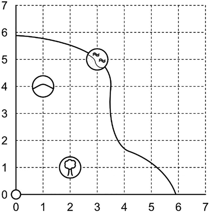
A grid graph plots a curve line with 3 marked landmarks. The tree is at (2, 1), the rocky hill is at (1, 4), and the sandy beach is at (3, 5). Values are approximate.
A map containing a few landmarks
Position and Direction Vectors
We can use vectors to represent the offset between our starting point and each of those three locations – the vector between our starting point and the tree is (2, 1), because it’s two miles to the east, or the x-direction, and one mile to the north, the y-direction. In fact, vectors are great at representing the offset between any two points simply because that’s what a vector is: a quantity that has a length and a direction. That’s the one-line description almost every textbook gives, at least! In this example, the direction is pointing toward the tree, and the length is about 2.24 miles. You might have noticed that the vector starting at the rocky hill and ending at the sandy beach is also (2, 1).
There are a few things to grasp already. Firstly, we can represent any position using its offset from some origin point, which in 2D is (0, 0) – that’s why I conveniently chose that as the starting point on our map. A vector containing only zeroes is always special, as it’s the only vector with a length of zero and without a particular direction – both properties will become relevant as we explore operations on vectors. It’s got a special name too: the zero vector. Secondly, vectors can start at any point on the map. Not only are they useful at telling us where some point is in relation to the origin point but they can tell us about the displacement between two points that are not (0, 0). This is important because saying “the vector (2, 1)” could mean several different things on the same map.
Vector Addition and Subtraction

A grid graph plots a solid line. The journey point starts with a point vector from the origin (0, 0) and goes to the point (1, 4), and ends at (2, 1).
The first leg of the journey
Vectors can easily be added to one another by taking each of the numbers inside the first vector and adding them to the corresponding numbers from the other vector (although both vectors must have the same dimension). Each of the values inside a vector is called a component, and they’re named like the axes of a graph: the first is the x-component, then y, then in higher dimensions z, and then w. Adding two vectors in 2D, then, is just a case of adding the x-components together and then the y-components. To figure out our position vector on the beach, let’s add up the components of the journey we took.

The sandy beach is indeed at (3, 5). Subtraction works the same way. We found a clue on the beach that’s directing us toward the tallest object in the area, so we’ll head over to the tree next – amazingly, there’s a perfectly straight concrete path that passes just by the tree. Whoever built these paths sure knows how to set up contrived math questions. Given the beach is at (3, 5) and the tree is at (2, 1), what’s the vector from the beach to the tree?
Remember that vectors have direction. We can get the answer by taking the destination vector and subtracting the starting vector. The same logic applies here: apply the subtractions component-wise.

In the context of our map, the vector (−1, −4) means “–1 miles east and –4 miles north” or, more simply, “one mile west and four miles south.”
Scalar Multiplication

A grid graph plots a solid line with 3 landmarks. The journey point starts from the origin (0, 0) and ends at (3, 5) and (2, 1) with a vector of 2 points.
Point vectors for the start and end positions of the next leg of the journey

This is an example of multiplication by a scalar. If a vector has several components, then a single number by itself is called a scalar, and they are helpful when it comes to vector math. Multiplication can be used to change the length of a vector – for example, multiplying the vector (2, 1) by 3 results in the vector (6, 3), which is three times longer, and multiplying by 0.5 instead results in (1, 0.5), which is half as long. Multiplying by 1 always results in the same vector; for that reason, 1 is called the multiplicative identity, just as the vector (0, 0) is the additive identity. Multiplying a vector by –1, like we just did, will always reverse the vector’s direction but preserve its length. Multiplying by other negative numbers will reverse the direction, but the length will change. And multiplying by 0 always results in the zero vector, which we discussed before. Dividing is the same thing as multiplication – just multiply by the reciprocal instead.


Vector Magnitude

A grid graph plots a right angled triangle. Its vector is represented by (2, 1), and the two other side lengths of 1 and 2 are used to calculate the longest side length.
The longest side length of a right-angled triangle can be calculated using the other two side lengths
You’ll likely be familiar with the Pythagorean Theorem, which is exactly what we use to calculate vector length (or, as it’s often called, magnitude). I’ll use the terms length and magnitude interchangeably throughout the book. With vectors, we’ll take the square of each component of the vector, add them together, and then take the square root of the result. We represent magnitude of a vector in formulas by putting vertical bars around it. So, for the vector (−2, −1), its length is represented by ∣(−2, −1)∣ and calculated like so:

So there you have it: when your teachers said Pythagoras would be useful in later life, this is what they meant. Now we know that the last leg of our treasure hunt was about 2.24 miles long, which is quite the trek. In fact, the total distance we walked throughout the day was 12.72 miles, so I hope we can afford a shower and a long rest using all that treasure.
Vector Normalization

A grid graph plots two point vectors at (0, 5) and (0, 1) with lengths of 5 and 1, respectively.
A vector of length 4 and its normalized counterpart, which has length 1
To normalize a vector, all we need to do is divide by its magnitude; we’ve seen how to do each bit before, so let’s put them together. I’m going to start with the vector (3, 4), which I’m going to call A. The corresponding unit vector is denoted  .
.

If we were to relate this back to the treasure hunt, then if we had set off from base camp toward the hill at (1, 4), got tired after exactly one mile of walking, and took a rest,then we’d be at  .
.
Basis Vectors and Linear Combinations
So far we’ve been discussing the properties of the vectors themselves, but now it’s time to talk about the map as a whole. Earlier, I mentioned that there are infinite vectors that point in the same direction as a given nonzero vector, but what does that mean? Our map is in 2D, and as a physical object, it will have a certain size. Let’s imagine the map extends infinitely in each direction. We can represent any position on this infinite map using a real number in each of the vector’s two components. We call the map a vector space (in fact, this space in particular is called ℝ2 because it’s two-dimensional and it’s made up of real numbers, ℝ).
In many contexts we’ll see throughout the book, it will be useful to represent position vectors as a combination of vectors that are perpendicular to each other. For example, the point (1, 1, 1) in 3D (in the space ℝ3) can be obtained by adding (1, 0, 0), (0, 1, 0), and (0, 0, 1) together. We say that the vectors (1, 0, 0), (0, 1, 0), and (0, 0, 1) form a basis for the vector space ℝ3, because these three vectors have the following properties: they are linearly independent, because we can’t add multiples of any two of those vectors to form the third one; and they span the entire space, because we can form any vector in ℝ3 by combining multiples of these three vectors. We may not use these terms very often in computer graphics, but we will see how sets of perpendicular vectors become important in later sections.
Dot Product
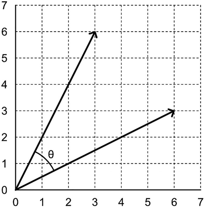
A grid graph plots two point vectors with origin at (0,0) and the angle between two vectors is theta.
The angle between two vectors
There are plenty of contexts where the angle between two vectors becomes useful, such as lighting, where the angle between a light ray and a surface normal vector influences the amount of illumination falling on the object. In these contexts, we use an operation called the dot product, denoted by a ⋅ b for the vectors a and b.


Recall that ∣a∣ and ∣b∣ are the magnitudes of a and b, respectively. θ is the angle between the two vectors. There are two ways of calculating the dot product, and both ways result in a scalar value. Neat! For that reason, the dot product is sometimes called the scalar product. So what can we do with the dot product? Well, it provides an extremely efficient way of evaluating the angle between two vectors. If we combine the preceding two formulas and rearrange them, then we have a good way of calculating the cosine of the angle between the two vectors.


We can evaluate the angle between the two vectors using just the cosine of the angle. For instance, if cos θ equals zero (and therefore if the dot product equals zero), the two vectors are at right angles to each other – they are perpendicular. In the lighting example I mentioned previously, the amount of light would be zero. Else, if cos θ equals 1, then the two vectors are parallel – they have the same direction. –1 means they are still parallel but point in opposite directions. We can see this if we calculate the dot product between (2, 1) and (−2, −1):


Any values of cos θ between 0 and 1 mean θ is between 0° and 90°, and when cos θ is between –1 and 0, θ is between 90° and 180°. However, you will notice we had to do quite a bit of rearranging to get a formula for the cosine. What if we could avoid needing to do that? You’ll see that the denominator in Equation 2-8 relates to the length of both vectors – if that equals 1, then the dot product is exactly equal to the cosine. We have already seen a method for making sure the input vectors have a length of 1: normalization! In many of the operations we’ll be doing throughout the book, it will be important to make sure all vectors are normalized first so that we don’t need to divide after doing the dot product. Since normalization involves dividing by the length anyway, this will only be more efficient if we use the dot product on the vectors more than once, but it’s a good habit to get into regardless.
Cross Product
We’ve seen a type of vector multiplication that results in a scalar value. What if we wanted to get a vector result instead? What would that look like? Enter the cross product, also known as the vector product. For two vectors in 3D space, the cross product between them will produce a third vector, which is perpendicular to both original vectors. There are a few caveats. Firstly, the cross product of any vector with the zero vector always results in the zero vector – perpendicularity isn’t well-defined for the zero vector. Secondly, the cross product of a vector with any vector parallel to it (including itself) also results in the zero vector. In this instance, there isn’t a single direction perpendicular to both input vectors – in fact, there are infinite directions such a vector could point in. Also, the cross product isn’t defined in 2D because you can never obtain a third vector perpendicular to both input vectors. For two vectors in 3D, the cross product looks like this:


In the first equation, n is the unit vector perpendicular to both a and b, and θ is the angle between a and b. A useful property of the cross product equation is that if both a and b are unit vectors and are themselves perpendicular to one another, then ∣a∣, ∣b∣, and sin θ all equal zero, and the equation becomes a × b = n. In most cases when calculating the cross product inside shaders, we can just normalize the output if we are certain that the resulting n is not the zero vector.
Matrices
We have seen how vectors work, but they are not expressive enough for us to carry out every operation that computer graphics demands of us. To get the best performance out of our graphics card, we will be using matrices for some of the most expensive calculations in the graphics pipeline. Let’s start with the most obvious question: what are matrices?
A matrix (the singular form of the word – the plural is matrices) is a rectangular array of numbers organized into rows and columns. They can have any size, and we refer to the matrix size by saying a matrix is m by n, where m is the number of rows and n is the number of columns. They’re kind of like tiny Excel spreadsheets.

Each number inside the matrix – each element of the matrix – is usually a real number in shaders. Matrices are usually denoted by a capital letter (in this example, we have matrices A and B), whereas individual matrix elements are denoted by a lowercase letter and subscripts to indicate which row and column of the matrix an element is from. For example, a1, 2 is the element of A in the first row and the second column, which is 4. b2, 1 is in the second row and first column of matrix B, which is –8. Unlike many programming languages, matrices are one-indexed – sorry.
As we will see later, matrices are used heavily in computer graphics to represent transformations required for taking data from a mesh and converting it into positions on-screen. If you are writing basic shaders, it is not necessary to know how each and every matrix operation works, because Unity will provide helper functions for us – in which case, you might wish to skip to a later section on space transformations to see how matrices generally help us in the computer graphics pipeline. However, some of the shaders we will see later rely on matrix operations, so I believe it is still useful to understand how to manipulate matrices ourselves.
Sometimes, it takes a while for matrices to stick in your brain if it’s your first time using them. If you need extra worked examples or if you’d like to go further with matrices than this chapter does, then cuemath.com/algebra/solve-matrices/ is a great resource.
Matrix Addition and Subtraction
There are many operations we can do with matrices, so let’s start with the basics. The size of the matrix is crucial because some operations become incompatible between matrices of certain sizes. Let’s take addition as an example. To add two matrices, they must be the same size. Adding is simple – just take each element from the first matrix and add it with the element in the same position from the second matrix.

Subtracting two matrices works in a similar way – both matrices must be the same size. We can think of subtracting a matrix as adding the negative of that matrix; finding the negative of a matrix is as easy as negating each element of the matrix.

Scalar Multiplication
Just like we could with vectors, we can multiply a matrix by a scalar value. We take every element of the matrix and multiply each one by the scalar value, resulting in a new matrix the same size as the original one.

This is called scalar multiplication. We will see how matrix multiplication works in a bit, but first, let’s look at some operations and terminology that are unique to matrices.
Square, Diagonal, and Identity Matrices
We saw how matrices are rectangular, but there is a special type of matrix called a square matrix, where there is the same number of rows as columns, such as a 2 × 2, 3 × 3, or 4 × 4 matrix. A diagonal matrix is even more special – it is a square matrix where every element must equal zero, except the elements on the diagonal line from the top left to the bottom right (this is called the leading diagonal). The elements on the leading diagonal could still equal zero. We’ll see later that these kinds of matrix have different behavior under certain operations.

An extremely important kind of matrix, the identity matrix, denoted I, is a diagonal matrix where all elements on the leading diagonal equal one. There is only one identity matrix for any given matrix dimension – here are the 2 × 2, 3 × 3, and 4 × 4 identity matrices:

Matrix Transpose
These are all interesting types of matrices, but let’s see some other matrix operations. First, there is the matrix transpose operation, denoted with a superscript T, such as AT (sometimes A′ is used), which effectively mirrors the matrix in the leading diagonal (remember – this is a diagonal line that starts in the top-left corner). The element a1, 2 in the new transposed matrix is equal to element a2, 1 in the original matrix. For the matrix A, which was 2 × 3, the matrix AT is 3 × 2.

There are a few properties of the matrix transpose operation to note. The transpose of the transpose of a matrix will return the original matrix. This makes sense – if we mirror a matrix in the leading diagonal and then mirror again, we expect to get back what we had originally.

We also find that if we add two matrices together and then take the transpose, the result is the same as if we had taken the transpose of the two matrices individually and then added them. Intuitively, this also makes sense if you think of the transpose as just moving the matrix elements to a new position: it doesn’t matter if we add elements and then move them or if we move elements and then add them – we are still adding exactly the same elements together.

If we multiply a matrix by a scalar value and then take the transpose, we get the same result as if we had taken the transpose of the matrix and then multiplied by the scalar. If you think about this in the same way as the previous example involving addition, the transpose is just moving elements around, so we are multiplying the elements by the same value in either scenario.

Matrix Determinant
Transposing is not the only useful matrix operation of course! We can also calculate the matrix determinant, denoted det(A) or ∣A∣ for the matrix A. The determinant only exists for square matrices – those with the same number of rows as columns. We rarely need to calculate this ourselves, but I will include the process here for completion. Let’s start with the determinant of a 2 × 2 matrix:


There are a few methods for calculating the determinant, but we will use the Laplace expansion, which is recursive and uses the 2 × 2 matrix determinant as its base case. The process is like this: We will take any given column or row of the 3 × 3 matrix. Let’s choose the top row. For each element of the row, if we “cross out” the row and column containing that element temporarily, we are left with a 2 × 2 submatrix, which we will calculate the determinant of using the preceding equation. Then, multiply by the element you started with.
In our case, we will be left with three values: a(ei − hf); b(di − gf); and c(dh − ge). We will combine these like so: add the value corresponding to the leftmost element, then subtract the next one, and then add the last one. Therefore, the determinant of this 3 × 3 matrix is a(ei − hf) − b(di − gf) + c(dh − ge).
In fact, if we were carrying out this process for a 4 × 4 matrix, the same rules would apply: calculate the determinant of the submatrices you obtain through “crossing out” each element of the row, then add the first, subtract the second, add the third, and subtract the fourth. This + − + − pattern extends to any size matrix. Don’t worry too much about needing to remember all this – it’s helpful to know what’s happening under the hood, but there are shader functions that do this for you.
So far, we’ve looked at some great matrix operations, but none are quite as useful as the next one we’ll look at. This one is the backbone of the entire graphics pipeline, and without it, we would struggle to build an efficient method of transforming data onto the screen.
Matrix Multiplication

If we were to calculate A × BT, then this would work because A has three columns and BT has three rows. The resulting matrix will be 2 × 2. On the other hand, A × B is not a valid operation, because B only has two rows. Before even seeing how matrix multiplication works, we can already make an interesting observation: by the same rules, BT × A is also a valid multiplication, but it will result in a 3 × 3 matrix. Matrix multiplication is said to be noncommutative because the order of the inputs matters. This is different from multiplying real numbers, which is commutative – for example, 3 × 9 = 9 × 3. On the other hand, matrix multiplication is associative like real number multiplication – that is, for three matrices L, M, and N, it doesn’t matter which order we resolve the following chain of multiplications: L × M × N = (L × M) × N = L × (M × N).

How do we carry out the multiplication operation? Let’s calculate A × BT. We already know this will be a 2 × 2 matrix. To calculate the top-left element, z1, 1, we will perform a product of the first row of the first matrix with the first column of the second matrix. Similarly, the bottom-left element, z2, 1, is the product of the second row of matrix A and the first column of matrix BT. The product works by taking the first element of the row and the first element of the column and multiplying them, then moving across the row and down the column and adding their product, and so on until you’ve reached the end of both the row and the column, resulting in a single scalar value to put in the result matrix. In fact, it works the same way as the dot product for vectors that we saw earlier.

Earlier, I introduced identity matrices. Recall that an identity matrix is square and has ones down the leading diagonal, with zeroes everywhere else. If we multiply any matrix by an identity matrix, then it is left unchanged by the operation. It doesn’t matter if the identity is first or second (as long as the sizes are compatible).

One last property of matrix multiplication is that taking the transpose after matrix multiplication is the same as taking the transpose of the individual matrices and then multiplying in the opposite order.

Matrix Inverse
The final major matrix operation we will explore is the inverse of a matrix. I briefly mentioned that a matrix is invertible if its determinant is nonzero. But what is the inverse of a matrix? If we multiply a matrix, E, by its inverse, denoted E−1, then the result will be an identity matrix. The order of multiplication does not matter – an identity matrix is always the result, and it will have the same size as E. Let’s say that E is a 3 × 3 matrix.

And how do we calculate the inverse? For a 2 × 2 matrix, this is not too complicated to do by hand. It requires us to calculate the determinant first. Recall that the determinant of a matrix only exists if the matrix is square; this means that non-square matrices do not have an inverse. Matrices that do not have an inverse are also sometimes called singular or degenerate.

As you can see, we are dividing by the determinant of the matrix to obtain the result. Inside the matrix, we have swapped the positions of a and d and negated b and c. Let’s try an example.

And what about inverting a 3 × 3 or 4 × 4 matrix? Calculating the inverse gets longer and more complicated the larger the matrix is, and it’s not worth learning how to do it, since shaders provide a function to do this for you. I’ve shown you the example for 2 × 2 matrices because they are more manageable, but the process for 3 × 3 matrices and beyond will take a lot of space to explain with little payoff.
We have now seen the basic building blocks of math we will need for the rest of the book. Vector and matrix operations will form the building blocks upon which we will build the next bit of knowledge. So far, we have considered both vectors and matrices in a general sense, but now we are going to see how we can use both for purposes that are directly relevant to computer graphics.
Matrix Transformations
I mentioned previously that matrices are going to be powerful enough for us to use them in the graphics pipeline. Usually, we represent points (or vertices) in space using vectors. As it turns out, and as I have hinted toward slightly, we can consider vectors to be a special case of matrix, which has only one column or one row, depending on which way round it is written. We’ll call them column vectors and row vectors. With that in mind, it becomes possible to manipulate point vectors using matrix multiplications – there are certain operations we can represent easily using matrices, and we’re going to see how they all work, starting with scaling.
If you need an extra resource to get to grips with matrix transformations, then I recommend learnopengl.com/Getting-started/Transformations. Although the website is geared toward learning OpenGL, this section is applicable to learning computer graphics in general.
Scaling Matrices
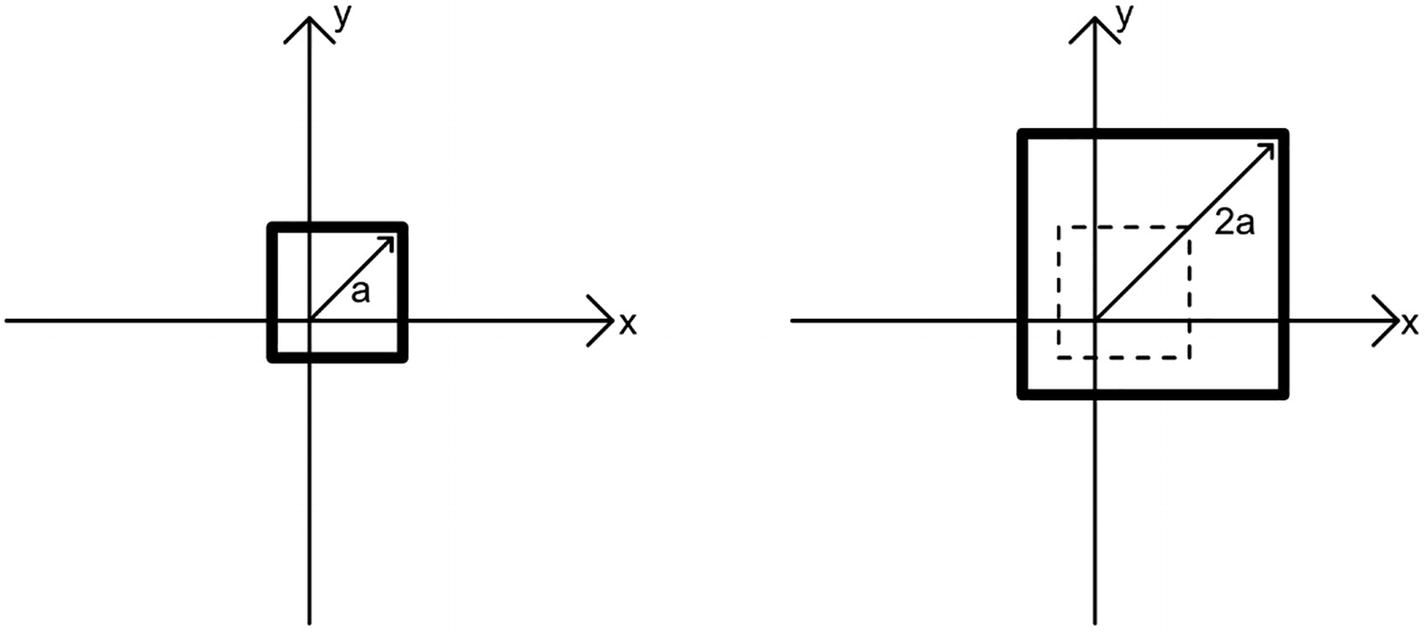
A graph with an X-axis and Y-axis represents the scaling up of a 2 D cube with the point vector by a factor of 2, with a uniform amount.
Scaling an object in 2D by a uniform amount in each axis
Of course, we can choose to scale in any of the x-, y-, or z-axis independently. Let’s say we have a vector v = (vx, vy, vz) that we want to scale in each axis. If we wish to represent this using just vectors, we can define another vector s = (sx, sy, sz) to represent the scaling factor in each axis (if we want to uniformly scale in all axes, then sx = sy = sz). Then, we can multiply the two together component-wise. This operation is called the Hadamard product, which isn’t often discussed alongside other vector operations – we’ll denote it as v ◦ s.

This is an efficient way to perform a scaling operation, but there’s a drawback: it’s not easy to combine this with other operations. In computer graphics, we often need to apply several transformations to an object at once (e.g., translation, rotation, and scaling). If we have a thousand vertices on our object, then we can do each of those operations one after the other on all vertices, or we can combine the operations into a single matrix via matrix multiplication and perform one pass over the vertices. The latter is far more efficient, and that’s why we use matrices. So how do we represent scaling using a matrix? If you recall, the identity matrix has ones down the diagonal. If we multiply a vector by the identity matrix, it is the same as scaling by 1. Hence, if we swap out those ones for other values, we can scale by different amounts.

Remember the rules for matrix multiplication: we have a 3 × 1 matrix (or column vector), and we wish to get another 3 × 1 matrix back out, so we need a 3 × 3 matrix for the scaling operation, and we need it to be on the left of the vector. I’ll note here that, for brevity, I’ve only described how to scale about the origin. You could, theoretically, scale relative to any point in 3D space, but the math gets a lot trickier. One trick we can use in this case is to translate all points in space so that the origin is now at the desired scaling point, perform the scale, and then undo the original translation (we will see how translation works soon). Of course, scaling is not the only transformation we can apply to vertices. Let’s also see how rotation works.
Rotation Matrices

A graph with an X-axis and Y-axis depicts the anticlockwise rotation of a 2 D cube around the origin at an angle theta.
Rotating counterclockwise by θ around the origin
Let’s see how a rotation around the z-axis works in 3D. A rotation around z will preserve the z-component of any point vector while changing the x- and y-components. A nice corollary of that fact is that any rotation in 2D can be thought of as a rotation around z, because you can think of 2D points as 3D points that have forgotten they have a z-axis (i.e., z = 0). If we wanted to carry out a rotation by angle θ around the z-axis, then conventionally the rotation would happen anticlockwise (or counterclockwise depending on where in the world you’re reading this), and it looks like this when working solely with vectors:

And, for completion, here are the similar rotations of angle θ around the y-axis and x-axis:


How would we represent these as matrices? As we can see, it’s trickier to work out than the scaling matrix was because each output vector component sometimes depends on multiple input components. For example, when rotating about the z-axis, if the input x-component is vx, then the output x-component is vx cos θ − vy sin θ. The rotation matrices, then, are not diagonal. In order, the rotations around the z-axis, y-axis, and x-axis by angle θ are represented by a matrix as such:


Take a few minutes to try out a few example rotations by yourself by multiplying a vector by any of these matrices. If you follow the matrix multiplication steps, take note of which calculations you’re doing – it’s the Hadamard product we saw earlier in the scaling step. And what if we wanted to rotate by angle θ about an arbitrary axis other than the x-, y-, or z-axis? Like we saw with scaling, we need to transform the entire world so that the desired rotation axis aligns with one of those three, then perform the rotation around that axis, and then undo the transformations we did in the first place. In this case, we can perform rotations around the x-axis by angle ψ and y-axis by angle φ to do the initial alignment such that the desired rotation axis lies on the z-axis, then rotate around the z-axis by angle θ, and then rotate around the y-axis by angle (−φ) and the x-axis by angle (−ψ). Let’s call the arbitrary rotation Rnew.

This is a great example of how matrix multiplication can help us. Instead of needing to perform each of these rotations on each and every vertex one after the other, we can combine all five rotations into a single matrix via multiplication like this so we only need to multiply each vertex by one matrix. Note the order of rotations – since matrix multiplication is commutative, we must put the matrices in this order. That said, matrix multiplication is associative, so it doesn’t matter which order we resolve each multiplication operation in once they’ve been written out like this. If we want to rotate about an arbitrary point other than the origin, then the process is like scaling – you can translate the entire space such that the arbitrary point lies at the origin, perform your desired rotation, and then undo the translation. On that note, it’s time to see how translation in 3D space works.
Translation Matrices
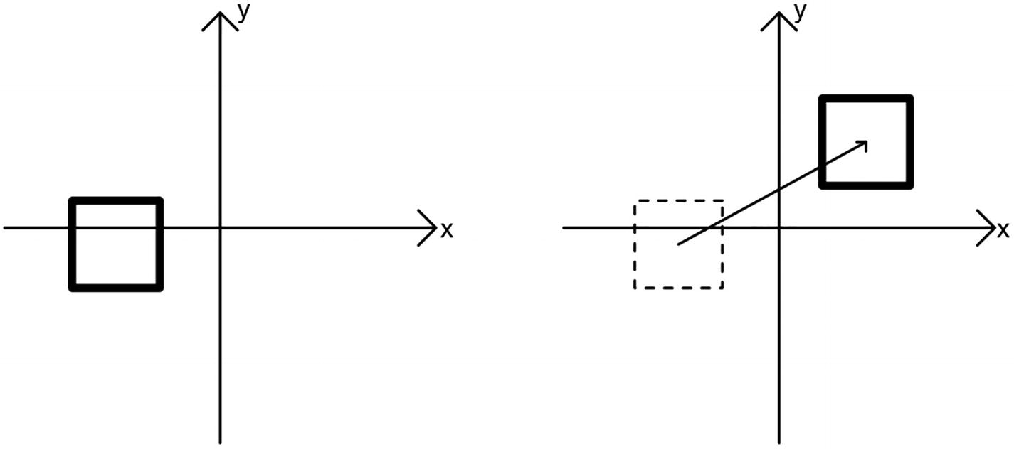
A graph with an X-axis and Y-axis represents; a 2 D cube at one location, and transforms a point vector to another location using translation.
Translation moves all vertices of a shape by the same offset
With vectors, this is very easy to represent using vector addition; if we wish to move a point vector v = (vx, vy, vz) by an offset t = (tx, ty, tz), then we can represent that like so:

Since it’s so easy to represent translation using vector addition, we can now go ahead and do the same thing we did with rotation and scaling and turn this into a matrix. But wait – we run into a problem if we try. With a 3 × 3 matrix, putting any value other than 1 along the leading diagonal will scale the points, which we don’t want, and putting any value other than 0 in any of the other positions means that the output value for one of the components will depend in part on the input value of a different component, which we also don’t want. That’s because the rotation and scaling matrices we wrote assume that we are rotating or scaling around the origin, but translation is moving the origin. Unfortunately for us, we really need to represent translation as a matrix operation if we are to harness the full benefit of using matrices, so we are going to need more information.
Homogeneous Coordinates
Let’s rethink the way we represent points using vectors. Right now, if we wish to represent a 2D point using a vector, we use a vector with two elements, x and y. For 3D, we add the component z. This is the most intuitive way to represent points (and directions) because we can separate out each component and see exactly where a point is along each axis. But this is not the only way of representing points. Let’s say we have the point (x, y, z) in Cartesian coordinates (the system we’ve been implicitly using until now). I could just as easily represent it using the vector (x, y, z, 1), which has four components instead of three. These are called homogeneous coordinates, and the fourth component is usually labeled w.
There are some quirks to using the new system over the old one. Firstly, any two vectors that are scalar multiples of one another represent the same point in 3D space. The vectors (1, 2, 3, 1) and (2, 4, 6, 2) represent the same point because each element of the second is twice the corresponding element of the first. This won’t be relevant just yet, but we will revisit this fact later. For now, all we will do is set the w component to 1. It’s also worth noting that we can get back to Cartesian coordinates by dividing each component by w and then removing the fourth component.
Now, what impact does this have on the hypothetical translation matrix? Since we are now using four-element vectors (which could be considered 4 × 1 matrices), we will need to use a 4 × 4 matrix. As we established previously, the translation values can’t be inside the upper-left 3 × 3 part of the matrix, and we have the added constraint that we need the w component to stay as 1 after the transformation. Let’s see what such a matrix looks like – I’ll include my working out for the intermediate steps.

Fantastic! Now we have a matrix for translation. Take a couple of minutes to step through each bit of the multiplication to understand why this wasn’t possible with just a 3 × 3 matrix. On that note, we won’t be able to multiply the 3 × 3 transformation matrices for rotation and scaling that we previously worked out by the new 4 × 4 translation matrix, because the sizes are now incompatible. We need to pad out the matrices with something – in each case, we add a fourth column and fourth row containing zeroes, apart from the lower-right element, which is always 1.


By now, we are armed with the basic knowledge we’ll need for tackling the computer graphics pipeline. It’s time to see how each piece of the puzzle we’ve seen so far fits into the pipeline as a whole and understand how the math we’ve seen helps us move data from one stage of the pipeline to the next.
Space Transformations

A three dimensional cubic object with 6 vertices and the object pivot (0, 0, 0). Three point vectors at the x, y, and z-axes are on the left side.
In object space, all vertices of the object are defined relative to the pivot point of the object

A cluster of 3 D cubic objects on the right side has individual object pivots and a camera. On the left, 3 point vectors at the x, y, and z-axes have an origin as world origin.
In world space, objects appear relative to a world origin point
Learn OpenGL has a dedicated section about coordinate transforms at learnopengl.com/Getting-started/Coordinate-Systems.
Object-to-World Space Transformation
Relating this to Unity in particular, each GameObject in your scene has a Transform component, which specifies the position, rotation, and scale of the object. The model matrix – the one that transforms from object to world space – contains each of these transformations inside a single matrix. Thankfully, we’ve covered each of these transformations already, so we will work through an example using what we learned previously.
We are going to transform the point v = (vx, vy, vz) by translating it by t = (tx, ty, tz) and scaling it by a factor of s = (sx, sy, sz), and, for the sake of simplicity, we’ll rotate only around the z-axis by an angle of θ (the real graphics pipeline can rotate around an arbitrary axis or perform multiple rotations). Matrix multiplication is noncommutative, so the order of each operation is important – which order should we do them in? In general, it shouldn’t matter if we are consistent. However, in this context, we know that the scaling and rotation operations assume that our point is relative to the origin, so it will be best if we leave the translation as the final operation. Let’s work through the example. Remember that we’re using homogeneous coordinates, so we’ll be transforming a slightly modified point v′ = (vx, vy, vz, 1).


We won’t only be transforming this single point, however. These matrices operate on every point in the mesh, but as I mentioned, we will multiply all the matrices together once and use that on every vertex. There is an extra wrinkle involved – what if the GameObject under consideration is a child object of some other GameObject? In that case, we can just evaluate from the bottom of the hierarchy upward: we apply the model for the object under consideration, then apply the model matrix of its parent, and so on until you reach the topmost object. This process can be optimized by calculating the model matrix for each GameObject only once and keeping it in memory, since the model matrix of any one object might be used several times.
Now that every vertex is in world space, let’s think about the next step. When rendering objects to the screen, we need some viewpoint within the world to use as our frame of reference, and we usually call this the camera. You can see it in Figure 2-11. Unity provides a Camera component we can attach to a GameObject for this reason; although we can have more than one, for the sake of simplicity, let’s assume there is only one and that it will render to the full screen. The next step is to transform everything relative to the camera.
World-to-View Space Transformation

A cluster of cubes from the camera's point of view depicts the object on the X-axis and Y-axis with individual object pivots.
A representation of view space from the camera’s point of view. Objects seen in this view have a z-position greater than 0. View space is like world space, but the origin is at the camera’s position. Not all objects represented here will necessarily be rendered
View-to-Clip Space Transformation
Game cameras come in two flavors: orthographic and perspective (although strawberry and chocolate would be better in my opinion). Each type dictates the shape of the view volume of the camera – in other words, objects outside this volume will not be “seen” by the camera.
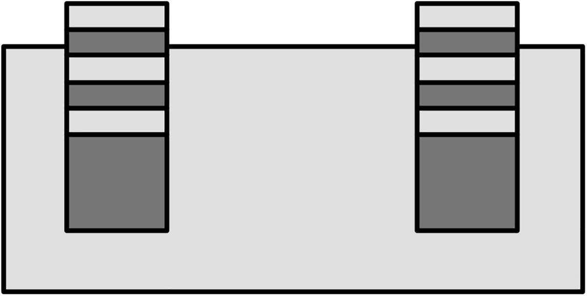
A rectangular plane has six lit cubes in repeating colors on each side at the top.
Six lit cubes on top of a plane, as captured by an orthographic camera

A rectangular plane has a linear arrangement of three lit cubes on each side.
The same six lit cubes on a plane, as captured by a perspective camera with the same position and orientation

A figure depicts; The changes in the camera's view space to the clip space; A cluster of cubes with box shaped dimensions, with inside objects as dark and outside objects as light colors.
Clip space places all objects inside a virtual box. Gray objects are inside the box; white ones are outside. Although the box dimensions are bounded between –1 and 1 in each direction, the box can still be a cuboid when visualized in world space. Objects are “stretched” to fill the clip volume
The projection matrix for an orthographic camera is constructed differently from one for a perspective camera. The orthographic variant is easier to create, and it looks like the following:


An orthographic camera captures the rectangular plane from the center with far clip and near clip distances.
A top-down view of an orthographic camera view volume
We can discern a lot about what the orthographic projection matrix is doing just by looking at it. On the right-hand side, we can see classic signs of a translation – this is repositioning each vertex such that the center of the view volume becomes (0, 0). The values along the leading diagonal represent a scaling operation such that the edges of the viewing volume are bounded between –1 and 1 in each axis. This matrix will also preserve the value of the w component of the point vector – if it is 1 before the multiplication, it will be 1 afterward.

A perspective camera captures an object in a view volume from the field of view with a far clip and near clip distance.
A top-down view of a perspective camera view volume
The perspective projection matrix is calculated like so:

Applying the perspective projection matrix also ends up with each vertex position inside a bounded box, but it must account for the field of view of the camera. We define the top, bottom, left, and right values relative to the vertical field of view (or FOV) in radians and aspect ratio using a bit of trigonometry like so:


The most interesting part of the matrix is that it will set the w component of the output vector to the z component of the input vector, which will be important later. For the first time, we will see values of w other than 1.
These transformations are the backbone of the vertex shader stage, which we will see in the next chapter, and there is another trick we can do to make the pipeline run as efficiently as possible. The view and projection matrices are based on the camera’s properties, which usually stay consistent while drawing a frame – that means we can multiply the two together. On top of that, the model matrix stays consistent for every vertex of an object, so we can multiply the model, view, and projection matrices together for drawing each object. The combination model-view-projection (MVP) matrix, as it’s called, is used in vertex shaders to perform all transformations in one fell swoop. It looks like this:

There is one last step after each transformation has been performed. We are still in homogeneous coordinates, so we need to transform back into Cartesian coordinates. At the same time, we need to collapse our 3D points onto a 2D screen.
Perspective Divide

A perspective camera and a screen are placed at z, equal to 0 and 1, respectively. Two points with the same coordinates are projected at different points on the screen.
Two points with the same (x, y) coordinates may not be projected onto the same point on the screen if they have a different z coordinate, due to the way perspective projection collapses points onto the screen (i.e., the z = 1 plane)
By dividing homogeneous coordinates by the w component, we end up with the vector  . Since we had previously set w = z, this is equivalent to
  , which puts all positions on the plane z=1, like we wanted. Once we have divided by w, we can ignore the last two components of the vector to end up with the final normalized screen position of the point: this is called normalized device coordinates, a 2D representation that maps the top edge of your screen to y = 1, the lower edge to y = − 1, the left edge to x = − 1, and the right edge to x = 1. The perspective divide happens automatically between the vertex and fragment shader stages.
Summary
Vectors can be used to represent points in any dimension.
There are many operations you can carry out on vectors, such as addition, scalar multiplication, normalization, dot product, and cross product.
Matrices are 2D arrays of numbers with a number of rows and columns.
Some matrix operations, such as determinant and inverse, only exist on square matrices. Some matrices do not have an inverse, and they are called singular.
Homogeneous coordinates add a fourth component to facilitate matrix transformations that would otherwise be impossible, such as translating 3D points.
A series of matrix transformations operate on vertex data, taking it from object space to world space, to view space, to clip space, and to normalized device coordinates.