
Chapter 3
Conducting an Onsite Site Survey
This chapter covers the following topics:
Performing a Walkthrough Survey: This section will help you assess the environment and discover, before the actual survey, areas that need special attention.
Performing a Layer 1 Survey: This section will show you how to detect non-802.11 transmitters, map their position, and assess their possible impact on your WLAN design.
Performing a Layer 2 Survey: This section will guide you through the site survey process, from the methodology to sample tools, for data coverage, voice or real-time application, and location deployments.
Performing a Post-Deployment Onsite Survey: This section will show you how to verify the deployment and make sure that the APs offer the performances projected during the pre-deployment survey.
This chapter covers the following ENWLSD exam topics:
1.3 Perform and analyze a Layer 1 site survey
1.4 Perform a pre-deployment site survey
1.5 Perform a post-deployment site survey
Once you have performed an offsite site survey, you likely have an estimation of possible access point positions and densities. Now, it is time to go onsite and perform an actual site survey. A common saying among wireless professionals is “you should do an onsite site survey every time you plan to deploy more than one AP.” This is because an offsite survey, although extremely valuable, cannot account for the realities of the environment and their influence on RF propagation.
However, you should not rush onsite with an AP on a tripod and start measuring cell sizes. The onsite survey process is composed of three phases, each of them aimed at saving your time for the phase that follows.
Therefore, this chapter will guide you through these different phases, starting with the walkthrough. This first phase can happen any time before the RF survey and aims at finding areas that will require particular care. These areas are often difficult to survey or likely to present challenges for your intended Wi-Fi coverage. The next phase is the actual survey, but its goal is not to design Wi-Fi cells. Rather, the Layer 1 survey phase is a critical step to determine the presence and position of any other RF transmitter that may affect your design or your future Wi-Fi coverage.
Then comes the actual Wi-Fi site survey that most experts refer to. In order for this phase to be fast, you need a systematic methodology, and this chapter will show you standard methods.
Last, once your network is deployed, you should go back onsite and verify the AP positions and configurations. You should also run specific tests to validate that the performance of the deployed network matches your design. This chapter will help you design and perform these tests.
“Do I Know This Already?” Quiz
The “Do I Know This Already?” quiz allows you to assess whether you should read this entire chapter thoroughly or jump to the “Exam Preparation Tasks” section. If you are in doubt about your answers to these questions or your own assessment of your knowledge of the topics, read the entire chapter. Table 3-1 lists the major headings in this chapter and their corresponding “Do I Know This Already?” quiz questions. You can find the answers in Appendix D, “Answers to the ‘Do I Know This Already?’ Quizzes and Review Questions.”
Table 3-1 “Do I Know This Already?” Section-to-Question Mapping
Foundation Topics Section |
Questions |
|---|---|
Performing a Walkthrough Survey |
1 |
Performing a Layer 1 Survey |
2–3 |
Performing a Layer 2 Survey |
4–5 |
Performing a Post-Deployment Onsite Survey |
6 |
1. A customer has hired you to site-survey a factory but asks that you skip the walkthrough to save time and money. What would be your position?
Walkthroughs are nice to have but can be skipped if the customer is familiar enough with the building.
The walkthrough can simply be performed after the actual survey.
Without a walkthrough, the survey will likely take longer and cost more money.
The walkthrough is needed but can be performed by a local factory worker to save on cost and time.
2. During your Layer 1 sweep in an office building, you find RF traces near a desk showing low power as well as multiple spikes across the 2.4GHz band. Which transmitter is most likely to produce this pattern?
A wireless security camera
An old 802.11b access point
A microwave oven
A Bluetooth headset
3. An engineer reports the detection of a DECT phone on channels 4 to 5 and wonders what is the best way to design around the interferer. What would you answer?
The phone may jump to other frequencies, and designing around it will be difficult.
As the transmitter does not affect channels 1, 6, and 11 that Wi-Fi uses, it can be ignored.
The admin needs to avoid channel 6 in this area.
The admin should set the nearby AP to channel 6 so as to cover the interference.
4. Your junior associate wants to start surveying a cubicle space in an office building. Where should the associate position the first AP to start the AP-on-a-stick survey?
At the corner of the building floor
At the geometric center of the floor
At the center of one cubicle block
Over the corridor between two cubicle blocks
5. You need to perform a site survey for voice and real-time application support. What is the correct way to proceed?
Perform a data site survey first. Then multiply the AP density by 1.3.
Perform a data site survey, using a phone to measure the AP signal.
Perform a voice survey, testing calls to evaluate each cell edge.
Perform a standard survey, using voice RF parameters.
6. Which of the following is a good way to confirm good roaming performance during a post-deployment survey?
Fewer than three channels scanned before the client associates to the next AP
50 ms or less between the last data packet on the previous AP and the first data packet on the next AP
30 ms or less between the probe request and the association request on the next AP
Less than 10 percent packet loss in the roaming area between APs
Foundation Topics
Performing a Walkthrough Survey
Before jumping to your site survey equipment, and often before even conducting the offsite site survey described in Chapter 2, “Conducting an Offsite Site Survey,” one of your first tasks is to go onsite and perform a walkthrough survey. This initial walkthrough is often a phase that is misunderstood by customers and networking professionals alike. You need to go to the site to survey, but without any site survey tool, just to assess what has to be done. The main purpose of the initial walkthrough may be summarized as “to answer questions that were not asked” (that is, to verify the required coverage by assessing the location with a professional look). Four types of areas can be identified, for each type of service needed (data, voice, or location, each with its relevant throughput target):
Areas where complete coverage and full performances are needed.
Areas where coverage is optional. Covering these areas is a plus, but no specific performance targets are set for these zones.
Areas where coverage is not needed. There may be some signal and partial coverage in these areas as a side effect of the deployment in other areas, but these zones are not to be covered.
Areas where coverage should not be present. There may be zones where coverage would be an issue. Typical areas may be parking lots, where visitors may try to eavesdrop or attack the network, research labs, and specific rooms in a healthcare environment, where the RF signal may disturb any existing Industrial, Scientific, and Medical (ISM) equipment.
Walking through the facility will allow you to identify precisely each of these areas. One additional benefit of the walkthrough is to verify the map you were provided. If the map is not recent, you may face unexpected surprises: wrong scale or wrong dimensions for some rooms, repurposed areas in which layout is now different from what the map indicates, or walls that were added or removed since the map was drawn. You do not need to verify the map and measure each room dimension down to the inch, but a quick look and comparison between what you see and what the map indicates will alert you if anything does not “look right.”
Verifying the areas to cover is also an important objective. In most cases, your customer will have indicated on a map the zones where coverage was needed. This indication takes the form of a line surrounding the area to cover. This coverage area definition is usually not very precise, and many details are often left to be determined. For example, do you need to cover the stairwell? For data coverage, this type of area is typically optional. For voice coverage, users commonly expect to be able to place or receive a call while transiting between floors, and stairwell coverage, along with efficient roaming from the main floor area (stairwells often feature a heavy firewall door) is a must. This notion of roaming path is critical for the walkthrough survey. As you design AP positions, you will find that observing a map blueprint is not sufficient. You need to be onsite and observe the floor layout and people’s behavior. You will see that people often use shortcuts through empty meeting rooms, avoid walking through certain areas (for example, open spaces where the local culture discourages disrupting people’s work by walking through). These observations will cause you to rethink roaming paths and best AP positions.
User behavior is also critical when examining user density. From a map, you may see cubicles. But are users using wired connections for all of their devices and performing basic browsing tasks, or are they on the other end of the spectrum, in an all-wireless office, using wireless headsets, taking voice calls, and pacing around? Are the cubicle walls thin or thick? Are they high or low? Can you cover the area from one AP in the ceiling, or will you need a different strategy? The initial walkthrough will still be enough to alert you if the structure seems to be different from what the map indicated. A typical example is a sample area with plaster walls, whereas other areas, not to be surveyed, use thick glass windows instead of plaster walls. As a wireless professional, you immediately know that the multipath and absorption parameters will be very different in both areas and that they should both be surveyed. The map and your customer may simply see them both as “having walls.”
Another goal of the structure examination is to evaluate constraints on AP placements. In many cases, APs will be installed at ceiling level. Thick concrete will be likely to provide some degree of RF isolation between floors, whereas thin structure with wood beams will most likely let the signal bleed from one floor to the next. This may cause devices on one floor to roam to the AP on the upper or lower floor, and such roaming may affect your ability to isolate floors or construct simple roaming paths, forcing you to think in three dimensions instead of on a floor-by-floor basis. Additionally, in buildings with decorative ceilings, positioning APs at ceiling level may not be possible, or it may be very expensive because the APs would need to be hidden above ceiling level and the decoration recreated. Some buildings also have hard ceilings of painted concrete, and positioning APs may be difficult or impossible, especially if there is a requirement to hide the AP or the Ethernet cable. Thick walls may introduce the same concerns for cabling. Some of these walls may have been built at a time when asbestos was used for insolation. There may be additional costs required to simply bring the cable to the AP intended location. Some buildings have atriums or high ceilings, too far from the floor level to provide good coverage without directional antennas and the risk of power mismatch between the AP and the clients. Last, there may be areas that will require special access considerations for the site survey, and the walkthrough should help you identify them. For example, many industrial environments have hazardous areas, because of chemicals or moving machinery, that require you to wear special attire or be accompanied by personnel. Some areas may not be always accessible (hospital cleanrooms or surgical blocks, occupied bedrooms in a hotel, and so on) and will require careful access-window planning.
During the walkthrough survey, you can also spot devices that may require closer examination, such as DECT phones, wireless cameras, and so on. In general, any device that seems to communicate with radio waves should be noted, so you can research what they are and what frequencies they use. This recommendation also applies to any detected AP. You need to know why this access point is here and if it is intended to stay. If you are planning for a wireless network upgrade, you need to clearly identify the existing deployment. The walkthrough can also help you assess the type of antennas and access points in use, which may provide useful information on specific building challenges that were identified during the previous survey.
During the walkthrough, another important item to monitor is the existing wired infrastructure. APs and Wireless LAN Controller (WLC) will connect to switches. These may be part of the deployment or upgrade plan. If you are expected to reuse some of the existing equipment, you will need to check for port availability and Power over Ethernet (PoE) budget. The walkthrough is a great time to reconcile the network map theory with the Intermediate Distribution Frame (IDF)’s reality. Another concern is cable length. The distance between the switch and the AP should not exceed 100 meters (328 feet). Distances may be short when calculated on a map, but a building is a three-dimensional environment. By looking at the switch positions, you may realize that some areas will be out of range because of the added distance due to high ceilings, pillars, or other obstacles. This environment may force you to install some mesh APs or request additional switches, in both cases adding to the deployment cost.
At the end of the walkthrough, you should have a clear initial idea on the complexity of the survey, but also on special considerations relative to the building structure or its occupancy that will have consequences on your WLAN design. The walkthrough can be performed at the beginning of the site survey phase. However, identified special conditions may force you to get special authorizations or equipment, and these may take time. As much as possible, it is therefore preferable to perform the walkthrough early in the design cycle, to ensure that your surveying time onsite will be as efficient as possible.
Performing a Layer 1 Survey
Once you have good information about the building particularities, and after you have performed an offsite survey to estimate possible AP locations, you are ready to go back onsite and survey the RF environment. This phase does not start with AP placement but with an evaluation of the RF environment itself. During the walkthrough, you may have visually identified non-802.11 devices. There are probably others, and most of them are likely not visible. The best way to assess their presence, and their possible impact on your WLANs, is to walk throughout the entire location while scanning the RF environment for any energy in the frequencies you plan to use. This activity is called a Layer 1 sweep, because you sweep the Physical Layer (the RF itself) in the frequencies you plan to use, without caring about what modulation and what protocol non-802.11 devices send. All that matters to you is the amount of energy they send (that is, how much they are likely to disrupt your WLAN).
However, this likelihood may not be easy to establish from a single sweep. Some non-802.11 devices are intermittent transmitters, sending different amounts of energy at different points in time. Therefore, the tool you need to use for this phase not only needs to detect RF energy, but it should also be able to inform you about the type of energy detected. At least it should identify the interferer’s general type. At best, it will give you detailed information about the device, sometimes down to product name and characteristics. Armed with this information, you can evaluate the likely effect of the interferer on your WLAN. You can then decide if you can design around it or if you will need to find ways to remove it (for example, by replacing it with Wi-Fi-based equivalent objects).
L1 Sweep Tool Essentials
Many tools allow you to capture the raw RF and analyze the detected energy. These tools are grouped under the general name “spectrum analyzer.” Many of them are laboratory devices, with a high-precision scanner, and are fairly expensive. They also offer many functions that are not needed for a simple site survey. You will also find programs that can run on a laptop and that can connect to a specialized card or device. When choosing such a tool, keep in mind that an application that uses your laptop Wi-Fi card will necessarily be limited by the low-level filter implemented by the card manufacturer, attempting to discard non-Wi-Fi waveforms. The application will have to extrapolate from the noise that was admitted through the low-level filters to attempt to guess what interferer and what energy may have reached the card from the energy that the filter admitted. Such an application will therefore produce less accurate results than an application that mandates specialized hardware to capture the entirety of the energy. Tools that require such a card include WiPry-Pro Spectrum Analyzer, WiFi Surveyor, CommView for WiFi, and MetaGeek Chanalyzer. You do not need to be an expert in any of these tools, but understanding their basic principles will go a long way when you perform a survey or analyze a source of interference.
In particular, Chanalyzer has the advantage of being able to capture from a specialized USB card but can also connect to a Cisco AP running CleanAir and capture raw data detected by the AP Spectrum Analysis Engine (SAgE). Although such a setup may not be the easiest for a site survey (because it supposes an AP, and thus a switch and a WLC, that you will have to power and carry around), it is definitely a solution that Cisco professionals are expected to know about. To enable such a mode, you can keep your AP in a normal (Local) mode, but you will then only be able to see that AP channel. If you want the AP to sweep the entire band, you need to set your AP to SE-Connect (in AireOS from Wireless > AP > Select AP > General > AP Mode > SE-Connect, and in C9800 from Configuration > Wireless > Access Point > Select AP > General > AP Mode > SE-Connect).
Then, on Chanalyzer, use the CleanAir menu and select Connect to CleanAir AP. Enter the AP name, the NSI key, and choose the slot (radio 0, 2.4GHz, radio 1, 5GHz or Monitor, to observe both radios) that you want to observe. This Network Spectrum Interface (NSI) key is a hash found in the WLC, on the AP General tab that you used to switch the AP to SE-Connect mode (the NSI key is also available in that same tab, if you choose to use the AP in local mode) and that encrypts the information exchanged with the AP. This method prevents eavesdroppers from intercepting and observing your exchanges with the AP. As you click Connect, you will see the energy reported by the radio(s) appear in the Chanalyzer GUI.
Whether you use Chanalyzer with an AP or a local module or another spectrum analyzer tool, you need to master some common concepts. The energy reported is commonly expressed in decibels. The decibel measures the power of a signal as a function of its ratio to another standardized value. The abbreviation for decibel is often combined with other abbreviations in order to represent the values that are compared. In the world of Wi-Fi, where energy is commonly expressed in milliwatts (mW), you will see the symbol dBm, representing the power level compared to 1 milliwatt (mW). A 0 dBm value is the same amount of energy as a direct 1 mW current. This would be an extremely high amount of energy for Wi-Fi. In most cases, you will see negative numbers (for example, −70 dBm and −80 dBm). On this negative scale, −80 dBm represents a smaller amount of energy than −70 dBm. The dBm scale is also used to express AP powers. For example, an AP set to a 1mW power level (this is pretty low) is set to a 0 dBm power level (because 1 mW is exactly the reference value, nothing more or nothing less). An AP set to 10 mW is set to 10 dBm, and an AP set to 20 mW is set to 13 dBm (10 dBs to get from 1 mW to 10 mW, then twice that power [that is, + 3 dB] to get to 20 mW; always start with the tens, then the threes).
When you compare two amounts of energy, expressed against the same reference unit, you remove the reference unit and only use the decibel term. For example, comparing interferer 1 detected at −70 dBm to interferer 2 detected at −80 dBm, you can say that interferer 2 is 10 dB weaker than interferer 1. The “milliwatt” symbol would not make sense here, as you are not comparing the energies against the 1 mW reference point, but you are comparing the interferers against one another. They happen to both be detected and measured against the mW reference point, but interferer 2 is 10 dB weaker than interferer 1, regardless of the unit against which they were measured. It is for the same reason that the signal’s received signal strength indicator (RSSI) is expressed in dBm (compared to the energy obtained by receiving a direct 1 mW current), but the signal-to-noise ratio (SNR) is expressed in dB, because you compare the signal to the noise (not to the effect of a 1mW current). This comparison only makes sense if both signal and noise are expressed in the same unit (dBm), but their relative strength is independent from the unit in which they are both expressed.
The decibel scale is logarithmic and therefore its scale is not linear. An easy-to-remember rule is that adding 3 dB doubles the power. Removing 3 dBs halves the power. Adding 10 dB multiplies the power by 10 (and removing 10 dB divides the power by 10). This rule is an approximation, but it is sufficient to compare powers you measure. Thus, above interferer 2 is 10 dB weaker than interferer 1 and therefore 10 times weaker. If interferer 3 is detected at −76 dBm, it would be four times weaker (70−3 to get “twice,” and −3 again to get “four times”) than interferer 1, and a bit more than twice as powerful as interferer 2 (they are 4 dB apart, whereas “two times” would be 3 dB apart). This scale logic is valid irrespective of the unit you are comparing against (strictly dB, dBm, or dB measured against another reference).
Therefore, the amount of energy detected from each interferer will be presorted in your spectrum analysis tool with the power at which the energy was received (in dBm) and the frequency (in the spectrum) where the energy was detected, as shown in Figure 3-1. It is clear that a stronger signal will likely affect your WLANs more than a weaker signal. However, the effect is a bit more complex. Most RF devices send bursts of energy and then stop. For example, your Wi-Fi card will send a frame and then stop. Even within the frame transmission, your card sends small bursts of energy of slightly different intensity, to represent the 0s and the 1s. The complexity of this variation depends on the signal modulation (for example, BPSK or QPSK, DSSS or OFDM, and so on). The same logic applies to any RF transmitter. Therefore, your spectrum analyzer will also report another metric called the Duty Cycle. This metric shows, within each second, what the percentage of time was when the interferer was detected. If the interferer was detected for 20 ms over each second interval, then its duty cycle is 2 percent (1,000 milliseconds divided by 20). The interferer may have a strong energy (high reported dBm), but it will affect your network only 2 percent of the time. This may be less disrupting than a weaker interferer present 60 percent of the time. In the end, there is a fine balance between power strength and the amount of time where this power was detected that will determine the impact of the interferer on your WLAN. Smart spectrum analyzer tools will give you guidance on how to evaluate these metrics together. Most tools will also allow you to display the average amount of energy, the maximum amount observed, or a real-time plot. The plot is often called FFT, for Fast Fourier Transform, which is a method to represent the captured energy in both the frequency domain and the time domain.

Figure 3-1 View of a Wireless (Non-802.11) Camera in MetaGeek Chanalyzer
NOTE
The 20 ms in our example may be grouped in a single burst or over many small bursts. Here, your ability to measure the duty cycle depends on the speed at which the spectrum analyzer card sweeps the band, and how granular it makes measurements. This is where the card price starts to matter, and you will read about resolution and rate. The resolution represents the amount of frequency, the channel size, that the card is able to capture at a time. If the card only captures 1MHz at a time, it may not see very narrow signals within that range (for example, a 12kHz signal), because they are too small to be distinguished from larger transmitters in that same chunk of the band, if both are transmitting at the same time. Therefore, a card with a good resolution will capture small chunks of band (for example, 72kHz) so as to be able to detect reliably narrow transmitters, even if they are sending energy in the same frequency as another larger transmitter. However, if your card needs to scan a 20MHz Wi-Fi channel, capturing only 72kHz may mean that the card might take a long time to sweep the entire channel, and its evaluation of the duty cycle may be coarse. The card may report a 10 percent duty cycle, but if it swept the channel once per second and averages over 10 seconds, its report will be less reliable than if it swept the channel 10 times during the last second. Therefore, cards will report the sweep rate, which is the amount of time in which they can sweep each chunk of frequency per second. This ability may depend on the width of the channel, and you may read metrics such as “10 sweeps per second over 40MHz.”
Interferer Types and Effects
You do not need to be an RF expert to pass the CCNP exams. However, there are a few very common interferer types you will encounter often during your surveys. While managing your networks, you will also see them often in your WLC Monitor page or in Cisco Prime Infrastructure (see Chapter 16, “Monitoring and Troubleshooting WLAN Components,” for more details on interferer management in deployed networks). In fact, they are so common that tools like Chanalyzer display their wave form in the main Interferers window. At the bottom of Figure 3-1, you see the shape of an 802.11b signal and the shape of an OFDM (802.11g/a/n/ac/ax) signal. A 20MHz-wide signal is shown in the 802.11g/n section. In the lower left part of the picture, you see a flat and wide signal, representing the same OFDM signal over 40MHz, as shown, along with other signals identified in Chanalyzer, in Figure 3-2.

Figure 3-2 Well-Known Signal Types in MetaGeek Chanalyzer
802.11 transmitters are reported but are typically not considered as non-802.11 interferers. However, the following interferers are also common:
Bluetooth: Present in 2.4GHz, BT transmitters are typical because of their spikes. There are frequency hoppers (they hop frequently between narrow channels spread across the entire 2.4GHz band). They are often low power. Many Bluetooth devices, or one very loud Bluetooth device, will negatively impact the wireless network. BLE (Bluetooth Low Energy) devices have an advertisement mode where only three channels outside of Wi-Fi channels 1, 6, and 11 are used. With BLE, you will see only three spikes until a connection is established, where all BT channels come back in use.
Video cameras (and A/V transmitters): These transmitters become less and less common, as more cameras tend to use Wi-Fi. They are still present on the lower end of the video surveillance market. These cameras typically allow up to four channels that partially overlap with Wi-Fi channels in 2.4GHz, as show in Figure 3-1 (two cameras, affecting channels 4–5 and 8–9). Being continuous transmitters, their effect on Wi-Fi is typically severe.
Narrow transmitters: In this category, you will find cordless phones, soundcast audio, and ZigBee. These transmitters use different protocols, but their channel is typically narrow (5MHz) and their Fast Fourier Transform (FFT )plots look similar, with a different signal strength. They all operate in the 2.4GHz band. Although some of these transmitters may use a fixed channel, allowing you to design around them, they also often implement some smart channel operations and may jump from one channel to another. They are therefore usually highly disruptive for the neighboring APs operating on the same band.
Microwave ovens: Microwave ovens definitely interfere with Wi-Fi networks. The interference is short-lived but can be very complete. Microwaves typically impact channels 6 to 11, but mostly channel 11. Microwave ovens are prevalent in healthcare facilities. In many cases, older microwave ovens can be damaged and produce unhealthy levels of emissions. Leakage can be caused by a broken microwave oven door or simply by the seal being damaged or dirty.
Jammers: Although they should not be expected in normal networks, jammers are cheap devices and easily bought online. Their characteristic is a continuous signal with a high duty cycle across the entire affected band. They may operate in 2.4GHz or 5GHz. The presence of a jammer signal is reflective of an attack against your network. Many jammers operate in the 2.4GHz band because this band is categorized as Industrial, Scientific, and Medical (ISM) and can be used by any transmitter (under some relaxed regulatory conditions). Most of the 5GHz band is not ISM, which makes it less susceptible to interferences from non-802.11 devices. However, different countries have different rules, and you may see in non-ISM 5GHz channels devices that were designed for a country where such operation is allowed.
Surveying for Interferers
As you perform your site survey, your first task is to walk the floor with a scanner and document any interferer detected. As your spectrum analyzer tool will report the signal strength, walk around to attempt to locate each interferer location. You may not visually locate the device (especially if it is embedded in another object or behind ceiling tiles), but you can document the location where the device was detected with the loudest signal. Also document the device type.
At the end of the process, you should have a map of the interferers, along with their expected severity and transmission profile. You can then evaluate their zone of impact as well as whether you can design your channel plan around the interferers or need to discuss with the Wi-Fi project sponsor to evaluate if the worst interferers can be removed (swapped for Wi-Fi-enabled, or Wi-Fi-friendly, equivalents).
Performing a Layer 2 Survey
Once you know what channels are available, your next step is to perform a Layer 2 site survey. This term is used to contrast against the Layer 1 sweep of the previous section, but its real meaning is simply a Wi-Fi survey (that is, a survey where you will determine the position of each intended AP).
The Site Survey Process
Depending on your user density model, you may design small cells or large cells. You may survey for simple data coverage, voice coverage, location, or all of them. Chapter 6, “Designing Radio Management,” will help you make those decisions. However, regardless of your deployment model, the site survey principles are the same: Set a test AP to a target power level, enable all data rates and Modulation and Coding Schemes (MCS) (you will use your survey adapter to determine the data rate boundary), and then try to position the AP on the floor and estimate its coverage cell. If you use a Cisco AP, you can enable “Aironet IE” on the WLAN configuration. This allows your AP to send its name and power level in beacons and probe responses. Most professional survey tools can read these elements. They are very useful when you review your survey results.
In most cases, you will want to use a site survey tool. This tool allows you to upload a map of your floor, click your position on the map, and then capture the signal from one or all the detected APs. At the end of the process, the tool can display the resulting RF signal map. By moving APs around and combining such captures, you can evaluate the best AP position and density for your coverage intent. Several such tools exist. The main contenders are AirMag-net and Ekahau for professional surveys, but you will find many other products, including VisiWave, NetSpot, and MetaGeek Map-Plan. You are not supposed to be an expert in any of them to pass the CCNP exams, but some familiarity with AirMagnet or Ekahau Pro will go a long way in helping you understand questions about the general survey process.
All tools allow you to upload a floor map, define its scale, and also configure some target parameters, such as expected client count per cell or minimum cell signal or data rate. These elements are useful for the tool to define audio warnings where the matching thresholds are reached, thus helping you define cell edges more efficiently. Also keep in mind that you can perform two types of surveys:
With AP-on-a-stick (APoS), you position an AP (usually on a tripod) and test the signal from the AP. This test can be done by simply listening to the AP messages (beacons and such) or by associating the wireless network card with the selected access point SSID (service set identifier) and then sending and receiving RF packets to and from the access point. The second method is only useful if you need to increase the number of 802.11 messages exchanged with the target AP.
In a validation survey mode, the wireless network card does not associate to any particular access point or SSID. Instead, it simply listens to the 802.11 frames as you move through the site. At the end of the process, the site survey tool allows you to select which APs cell coverage you want to analyze.
Note
The validation survey is sometimes called a “passive survey.” The APoS survey is sometimes called an “active survey” (because you actively associate your adapter to an AP). However, these terms have different meanings in different tools. For example, in Ekahau Pro on a laptop, the Ekahau adapter (attached to your laptop USB port) never associates to an AP. However, you can use your laptop internal adapter to associate to the AP. If you do so, you can also activate an “active” mode to continuously ping the gateway, thus testing both the RF connection and the gateway connectivity performances at the same time.
You should start with the validation survey to assess the existing Wi-Fi environment before your deployment. This step is useful not only in detecting existing Wi-Fi APs on the floor of your survey but also in discovering neighboring networks and which channel plan and power level may have consequences on your design.
You will also perform a validation survey after your deployment is completed (to verify the coverage). During the initial Layer 2 survey phase of a new deployment, you will carry APoS surveys in most cases. The steps of this phase can be summarized as follows:
Determine the possible locations where an access point should be placed.
Place the access point in the most desirable location (APoS) and conduct as many surveys as needed to ensure that the access point intended coverage area is fully monitored, and that you did find the best location for that AP. In a survey tool, you may need to perform several surveys to examine the AP cell in multiple directions. Save the survey data at the end of each survey; you may end up merging (and associating) several survey data files for the access point at one location in order to get a full picture of the cell.
Repeat until the facility is covered.
Save the survey data at the end of each survey.
As your site survey should include overlaps between cells, it is best to use several access points in the process. Three APs is a common quantity. In places where carrying three APs is a challenge (each AP needs a power source, a pole, and so on, which adds to the overall volume of equipment to carry), you can use two or one access point instead. The difficulty in that case is to evaluate the overlap between cells.
To start your site survey, identify a large obstacle, such as the building edge or a large heavy wall through which signal will not bleed. Working from there, your job is to find the position of the first AP. Taking the edge of the building as an example, as illustrated in the left part of Figure 3-3, place the access point at location 1 to start. Perform a site survey to determine the signal strength of the coverage area. Mark where the data rate falls to the minimum acceptable value until you have traced a semicircular pattern on the floor, which will determine the coverage boundary. Move the original access point to a centrally located position on the coverage boundary 2, as shown on the right part of Figure 3-3, to create the first coverage area. The logic is that if you get coverage up to point 2 when the AP is at position 1, then you should get coverage down to point 1, which is the corner of the building, when the AP is at position 2. Position 2 is located along the coverage boundary determined when the AP was in position 1, preferably at equal distances from each building wall, which places the AP toward the center of the building.

Figure 3-3 The Site Survey Process—Positioning the First AP
Once the AP is moved to position 2, perform a site survey to determine the signal strength of the new coverage area. Mark where the data rate falls to the minimum acceptable value until you have traced a circular pattern on the floor that will determine the coverage boundary. This is the position where the cell application performance would decrease to the point where your client device will search for a better AP. However, you should also continue capturing the AP signal beyond that point to evaluate the RF footprint of the AP. This will help you evaluate areas where APs on the same channel may interfere with each other.
This position 2 is expected to be the final position of the AP for this zone, and the coverage area should represent the expected useful coverage (the zone where a client can actively and efficiently perform data communication with the AP) when the final AP is deployed at this position. You may have to move the AP if the measured coverage area does not match your expectation because of obstacles or interfering objects.
Now place another access point adjacent to the first coverage area to determine another coverage area with appropriate overlap of the two areas, as shown in Figure 3-4. Continue through the facility until all areas needing coverage are accounted for and you have acquired the appropriate overlap between cells for client roaming purposes.

Figure 3-4 The Site Survey Process—Positioning More APs
Keep in mind the cell edge and the cell overlaps. If you decide that the cell edge is at −67 dBm, then this design means that at the position where the client detects the AP at −67 dBm, the client can also detect another AP at −67 dBm or higher. This does not mean, of course, that the client will roam at that point. Each client has its own internal algorithm and threshold structure to decide on roaming points. However, this design means that, as the client continues to move away from the first AP, the next AP signal becomes even stronger. At any point in space and time where the client decides to roam as you keep moving, the next AP will offer a good signal, sufficient for the client to make a fast roaming decision. Also keep in mind that the AP RF footprint does not stop at that cell edge. In theory, the AP signal reaches infinity. Practically speaking, the AP signal will be detectable way beyond the intended cell edge. You should continue surveying the AP coverage until you have assessed the full AP footprint (that is, to the point where the AP signal reaches the noise floor, typically around −94 dBm in a standard building).
If you work in an open space, or if the wall structure is fairly homogeneous, you can use shortcuts. In open space propagation, a common rule is “6 dB = twice the distance” and “the first meter loss is at least 50 dB with omnidirectional antennas.” In other words, if you position an AP and set its power to 100 mW (20 dBm [that is, 10 dB to get from 1 mW to 10 mW, and another 10 dB to get from 10 to 100 mW]), you should expect at best −30 dBm at 1 meter from the AP (20–50). We say “at best” because imperfection in the antenna radiation pattern may cause the power to be even lower. Supposing an imperfect antenna and a signal at −36 dBm at 1 meter, you should then expect 6 dB less each time you double the distance (that is, −42 dBm at 2 meters, −48 dBm at 4 meters, −54 dBm at 8 meters, and so on). Keeping this ratio in mind can help you save time by converting distances into likely signal levels.
For example, suppose you deploy two APs in an open space. Suppose that you stand at the midpoint between these two APs, and you positioned them so that their signal reaches your client at −67 dBm at this position. If, from this point, you walk to any of the APs, you double the distance to the other AP (as you were standing midpoint). Therefore, that other AP’s signal should now be around −73 dBm, or −67 − (−6). This also means that if you deploy one AP and then stand at that AP position while a colleague moves away another test AP, you can be confident that the other AP is at the right distance when you detect its signal at about −73 dBm. This model is, of course, only valid in open spaces. In most buildings, however, you will find walls and obstacles on your path that will make this shortcut more complex to apply, but the same principles can be applied with small variations. Refer to Chapter 2 for a list of common obstacles and their attenuation.
A more cautious approach is to position each AP individually and then systematically walk the floor around the AP so as to precisely find the cell edge. In most professional site survey tools, you can choose to emulate a particular client type. Then, as you walk, you can see the signal level in real time (or the data rate, the SNR, or other RF quantity you need to measure) for your target AP. To draw the contours of your AP heat map, click where you are on the map, walk a few steps, and then click your new position (some tools allow you to click a starting and ending points, then walk at a steady pace in a straight line between these two points, without having to click intermediate locations). In the end, the tool will display the heat map of the detected AP. Most of the those tools will also attempt to position the AP automatically, assuming that the direction of the strongest signal is likely to point to the AP. After repeating this exercise with a few APs, you can combine the views in a single heat map, as illustrated in Figure 3-5 for Ekahau Site Survey Pro.

Figure 3-5 Ekahau Site Survey Pro
Click the Survey tab to start the data collection, and click the Planning tab to work with existing data or make coverage predictions. From this mode, you can move the APs (green circles on the map) if the tool incorrectly assumed their position. You can see the recorded path in green, with green points that mark the positions that were clicked on the path. The current view includes all recorded APs (called “My Access Points”). You can add or remove APs to or from this list as you try and then keep or discard different AP positions. As you will likely carry fewer APs than the entire floor will need for full coverage, you will probably have to rename each AP as you move it to a new position. At the bottom of the screen, a real-time view of the RF environment allows you to monitor the current detected APs along with their channel and RF characteristics.
As you design your network, keep roaming in mind. If you expect your users to move while connected, you need to ensure optimal roaming conditions. This means that the client should always detect the next AP while moving. This principle is illustrated in Figure 3-6. A user walks along the path from points A to B and then C. APs are represented as green points. On the left side, as the user, associated to AP 1, turns at point B and walks toward point C, the elevator banks (represented by squares with crosses) on each side suddenly obfuscate the signal from AP 1. The client may have detected AP 2 before deciding to associate to AP 1, but AP 2 is now also not detectable. As a result, the client needs to undergo a panic scan before discovering and joining AP 3. This creates disruptions during the roaming phase. By contrast, on the right side, the client can jump to AP 2, because that AP is still accessible on the B-to-C segment. As the client scans to discover and join AP 2, it also discovers AP 3, which will be a possible jumping point when the user reaches the end of the corridor.
This principle illustrates that the view from the ceiling should match the view from the floor. As your client moves between APs, your design should ensure that a client associating to one AP always has RF reachability to the next AP on the path (even if that AP is farther away and therefore not chosen by the client). This principle has to work regardless of the walking direction. As you will learn in Chapter 8, “Designing for Client Mobility,” the APs can send signals (using the 802.11v and 802.11k protocols) to help the client discover the next AP. This means that the APs visible to the client should also be visible to the APs (thus making the view from the ground the same as the view from the ceiling, as much as possible).
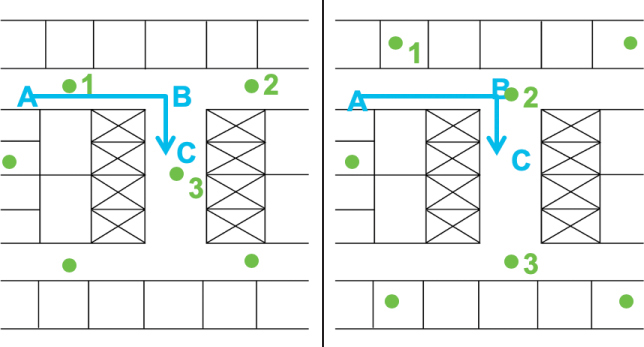
Figure 3-6 Positioning the Next AP
These general principles, along with the surveying method, should allow you to build your way through the floor, designing as you go to determine best AP location and AP density. At the end of the floor survey process, you should be able to build a complete view of the floor coverage by combining the heat maps of your different APs and their various expected best positions. You will use this outcome to produce a site survey report. This report lists the APs used, their power settings, channels, coverage target assumptions, and the expected resulting coverage heat map. This report will be used to deploy the APs. In most cases, it is also useful to take actual pictures of the spots (possibly marked with a piece of tape) where you project that the APs should be positioned.
Data vs. Voice vs. Location Deployments
The density of APs will depend on the application you intend to deploy. Data coverages are typically done with larger AP cells and low data rates at the edge, thus maximizing the cell size (and minimizing the AP count). Such deployment offers poor performance for time-sensitive applications (for example, voice). When designing for real-time applications, you will want smaller cells, with APs at lower power, so as to ensure that clients always have a high data rate. Chapter 5, “Applying Wireless Design Requirements,” will give you additional details on these various requirements. In all cases, the survey process is to choose the target signal level at the cell edge, choose a target minimum data rate for that cell edge, and then position APs to find the cell contours. Here are some points to keep in mind:
Start by deciding on the AP power level. This element primarily depends on the client type you expect in your cell. Most smartphones have power limited to 11 dBm or 14 dBm. Larger tablets and laptops can reach 16 or 20 dBm. If you know your target client, verify its capability. In most cases, the AP has a better receive sensitivity than the client, so you can set the AP power higher than the client. For a voice deployment, you can set the AP to 14 dBm, and 17 dBm for a data deployment. This value accounts for the fact that radio resource management (RRM) may be able to increase or decrease the AP power wherever needed.
Think redundancy. If one AP gets disabled, you will want RRM tools to dynamically compensate for the gap by increasing the neighboring APs’ power. Use the 6 dB rule to evaluate if you would still have coverage from neighboring APs, should one AP be disabled.
Decide on the expected AP signal level (as measured by the client) at the cell edge. For data coverage only, a typical target is −72 dBm. For voice, it’s −65 dBm to −67 dBm. As most indoor networks today expect to see voice traffic, −67 dBm is a good target.
Decide the minimum data rate allowed to that cell edge location. For basic data coverage, 6Mbps is common. For voice or real-time application support, 12Mbps is common, and 24Mbps is expected if real-time video applications (for example, video conferencing) are your target. Here again, as most cells carry both data and voice, designing around 12Mbps minimum has become common even for data-only support, in anticipation of occasional voice activity. To ensure this boundary, configure your site survey tool to stop displaying the heat map below your data rate target (when displaying the data rate view). Most tools can emulate the signal level at which each client would use a particular data rate.
Decide the minimum acceptable SNR for your cell. This parameter goes along with the RSSI and will dictate how close APs on the same channel can be to one another, as each AP will be a cause of noise (thus lower SNR) to the clients connecting to the other AP. A common value is 12 dB or more for basic data, and 25 dB or more for real-time applications.
Note
This SNR requirement means that if your cell edge is set to −67 dBm, at that position the noise floor should be at −92 dBm or lower, which is easily achieved in indoor environments. However, in high-density environments, you may have to position other APs in range on the same channel. In that case, the rule can be bent to 19 dBm isolation. This means that at the −67 dBm edge, the signal from the next AP on the same channel should be heard at −86 dBm or lower. This value is higher than the noise recommendation and is possible because the APs can recognize the 802.11 transmission and accommodate for it. This recommendation is for the next AP on the same channel. Of course, the neighboring AP will be heard much louder, as you want to ensure seamless roaming between APs. But that neighboring AP will be on a different channel.
These requirements are default templates for data and voice deployments. Your particular deployment needs may dictate different values. You will also find older recommendations that suggest to keep the 5GHz band for voice and real-time traffic and keep data in the 2.4GHz band. This scheme was valid at times when SSIDs were specialized (voice SSID, data SSID, and so on). Today, the same SSID carries all traffic. As such, you should design your WLAN in the 5GHz band, if it is allowed in your regulatory domain. Some deployments completely ignore the 2.4GHz band. Some others use it to carry IoT traffic (data from Wi-Fi sensors, with a different SSID than on 5GHz). Others use it as a backup, to allow coverage in zones where the 5GHz coverage may be weak. This logic is based on the fact that antenna sizes (for clients and APs) have a direct inverse relationship with the frequency of the signal. The 2.4GHz signal uses antennas about twice as large as the 5GHz signal, and therefore 2.4GHz transmissions appear to be about twice as powerful as 5GHz transmissions (as 2.4GHz antennas collect about twice as much energy as 5GHz antennas because they are about twice as large). A direct effect is that 2.4GHz cells expand to larger areas than 5GHz cells and can still provide coverage at distances where the 5GHz signal is too weak to be used. This gain is often accompanied by more noise, more interference, and more collisions, and this is why a larger 2.4GHz cell is only a backup in these scenarios. However, a 5GHz-only design is more common.
For location deployments, a few considerations need to be added:
Location uses trilateration, which means that you need several APs around each point of your floor so that a location engine in the infrastructure can combine the signal these APs receive from each client and compute the client location. For each point of the floor, you need at least three surrounding APs, in different directions (in different “quadrants”), and preferably four or more. At least three of these APs should be less than 70 feet (21 meters) away and should read any client signal coming from this point with a level of −75 dBm or more (−72 dBm recommended).
As much as possible, try to scatter the APs. In other words, do not set the APs in a long straight line. For example, in a hospital or a hotel where there are bedrooms and a central corridor, do not put the APs in a line in the corridor. Rather, try to position the APs in the rooms. This scatter disposition helps the trilateration computation.
As much as possible, try to create a “convex hull.” This means that there should be APs at the edge of the floor, so as to make sure that the first recommendation applies everywhere and that each point where location is needed is surrounded by APs. Deploying APs near the building walls may not make sense from a pure data or voice coverage standpoint. For this reason, the APs at the edge are often set to Monitor mode. In this mode, the APs do not support any client service, and they only receive the client signals. In most cases, you would perform a survey for data or voice and then add at the edge of the floor additional APs set to Monitor mode.
Do not put your AP antennas too high. As the antennas get higher, the minimum distance from the client to the antenna increases. All clients start to appear as “far” regardless of their actual position, and the location accuracy gets degraded. A common recommendation is to place the antennas no higher than 20 feet (6 meters) above the clients’ location. A typical ceiling height is 10 feet (3 meters), which is a good height. The maximum height recommendation is primarily intended for large indoor spaces, like warehouses or atriums.
These considerations are illustrated in Figure 3-7 and apply for location services based on RSSI (that is, when the infrastructure uses the client signal for location purposes). The convex hull is set for the upper part of the floor.
For other location technologies, like Fine Timing Measurement (FTM), Bluetooth Low Energy (BLE), and Angle of Arrival (AoA), other considerations may apply. Although these modes are too advanced for the CCNP exam, make sure to look up the vendor documentation if you plan on deploying these other location solutions.
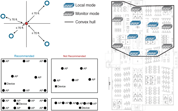
Figure 3-7 Location Deployment Recommendations
Performing a Post-Deployment Onsite Survey
Once your recommendations have been applied, there should be APs positioned on the floor at correct locations. However, deployment complexities are always possible (for example, A/C conduit behind a ceiling tile, preventing cabling from reaching your exact intended AP position). Additionally, you likely surveyed with a subset of the APs eventually deployed. Therefore, once installation is complete, you should always come back onsite and perform a post-deployment survey to verify coverage and performances.
Start by conducting a validation survey of the entire deployed environment (divided into several shorter surveys, if necessary) and compare the results to those generated during the pre-deployment survey. They should look nearly identical. Pay special attention to the areas that you identified, during the walkthrough or the survey, as difficult areas. These are typically areas where positioning APs and ensuring proper coverage are challenging (high ceiling, presence of strong multipath sources, and so on). A visual review of the deployment should help you identify those APs. The post-deployment survey will also reveal them by showing areas where coverage is inconsistent. In all these identified areas, perform a client performance test with a “poor” client, as defined later in this chapter, testing for the client and AP RSSI and SNR.
If the client performances do not match your expectations for those difficult areas, you may use several factors to mitigate the issue. One first and obvious possible action is to determine if the AP can be moved to a more “RF-friendly” location. In many cases, APs were deployed by insufficiently trained personnel, and the mis-location of the AP has no other cause than the installer being unaware of the detrimental effect of the environment on the AP performances. Relocating the AP may not be a major issue in that case. In some other cases, the AP location results from a conscious decision, based on aesthetical issues or other constraints, and the AP cannot be moved anymore. The second possible action is to work with the AP power level to help mitigate the performance issues. If the AP is behind an obstacle, manually raising the AP power level may help the AP signal get through the obstacle. Increasing the AP power level is not the best option, though, as “good configuration does not compensate for poor deployment,” as the saying goes. As you increase the AP power, you also increase the issues related to reflections and multipath. The result is that the AP signal may be stronger at the client level, but multipath issues may be worse. Increasing the power also does not change the AP Rx sensitivity, and your client link may become asymmetric.
Testing real applications, with a real client, allows you to verify that the real-world network traffic (for example, physical data rate, packet loss or packet retry, uplink or downlink data) meets user requirements. Survey by SSID and by AP to ensure that smooth roaming is taking place. Walk both sides of all access points to ensure you stay connected. This task should preferably be done with a typical client or the client expected to perform the most poorly. (“Most poorly” in this context means the client that displays the lowest performances.) This can be measured by positioning several clients next to one another, connected to the same AP. The client displaying the lowest RSSI from the AP and the lowest data rate is likely the best candidate for testing. You should also attempt to measure the performances of the application most sensitive to roaming delays. This is typically a real-time application (for example, voice). A good test procedure is as follows:
Associate with each access point in the WLAN.
Make stationary calls and verify the audio quality.
Verify that you can make roaming phone calls with good-quality audio and no disconnections.
Place multiple calls, especially in areas that are designated for high-density use.
Make sure to test and identify rate-shifting points. During your site survey, you determined roaming paths and know that wireless client data rates are going to shift down as clients move away from the access points. If your deployment uses delay-sensitive applications, you may want to test how going through these rate-shifting points affects the client performances. You probably will not test each rate-shifting point for each AP but will focus on specific areas where rate shifting might be an issue. Those are any areas where brutal rate shifting is expected. For example, if a roaming path goes through self-closing doors, you know that the data rate will shift down brutally as soon as the door closes (if the connected AP is still on the other side of the door). The same issue may occur at any location where a sudden change in the AP signal is expected. This change may be due to the physical layout of the facility (angle in a corridor, pillar or wall section between the client and the AP, and so on). The change may also be due to the environment (areas with sources of multipath, reflection, or interferences). For delay-sensitive applications, you may want to test those areas and verify the roaming delay in both directions to ensure that the user experience will be seamless even through those difficult areas. In some cases, you may have to reconsider some APs’ position or power level (for example, reducing an AP’s power in order to make the client attempt to roam sooner).
Note
You cannot manipulate the clients’ parameters. Most clients will start scanning for the next AP when the current AP signal falls below a target threshold. What you can do is measure the client behavior, determine the threshold, and set the AP to bring the roaming phase to an area where connection interruption will be shorter. Each client is different, but you will find common behaviors. For example, Apple iOS phones scan when the AP signal falls below −70 dBm. Samsung phones and most laptops (including macOS) scan when the AP signal falls below −75 dBm. Most clients need the alternate AP signal to be at least 6 to 8 dB better than the current AP to make the roaming decision.
As you test roaming, you can measure performances. Beyond measuring RSSI, SNR, and retries, the most accurate way to evaluate roaming efficiency is to measure the interval between the last data packet on the previous AP and the first data packet on the next AP. A roaming delay of 50 ms or less will likely not be noticed by any client or application. A delay of 100 ms may be detected by an audio application (causing one or a few packets to be lost and resulting in a short metallic texture to the sound or a click). Longer delays are obviously more impactful.
At the end of the post-deployment survey, you should be able to validate if the deployment matches your expectations. Document discrepancies so as to set correct expectations but also to plan for the next phase of the network lifecycle and future upgrades.
Summary
This chapter examined the process of an onsite site survey and its different phases. In this chapter you have learned the following:
How to perform a walkthrough survey to identify problematic areas
How to perform a Layer 1 survey and how to detect, map, and evaluate the effect of non-802.11 transmitters
How to perform a Layer 2 site survey for data, real-time applications, and location coverage
How to perform a post-deployment site survey and assess the network performances
References
For additional information, refer to these resources:
Cisco site survey guidelines:
VoWLAN site survey and validation: https://www.cisco.com/c/en/us/td/docs/wireless/technology/vowlan/troubleshooting/vowlan_troubleshoot/8_Site_Survey_RF_Design_Valid.html
Location-based services RF design: https://www.cisco.com/en/US/docs/solutions/Enterprise/Mobility/emob30dg/Locatn.html
Cisco WLANs for iOS design guide: https://www.cisco.com/c/dam/en/us/td/docs/wireless/controller/technotes/8-6/Enterprise_Best_Practices_for_iOS_devices_and_Mac_computers_on_Cisco_Wireless_LAN.pdf
Cisco 8821 design guide (coverage and redundancy recommendations): https://www.cisco.com/c/dam/en/us/td/docs/voice_ip_comm/cuipph/8821/english/Deployment/8821_wlandg.pdf
Exam Preparation Tasks
As mentioned in the section “How to Use This Book” in the Introduction, you have a few choices for exam preparation: the exercises here, Chapter 18, “Final Preparation,” and the exam simulation questions in the Pearson Test Prep Software Online.
Review All Key Topics
Review the most important topics in this chapter, noted with the Key Topic icon in the outer margin of the page. Table 3-2 lists these key topics and the page numbers on which each is found.
Table 3-2 Key Topics for Chapter 3
Key Topic Element |
Description |
Page Number |
|---|---|---|
Paragraph |
Perform a walkthrough survey |
46 |
Paragraph |
Layer 1 essentials |
49 |
Paragraph |
Interferer types and effects |
52 |
Paragraph |
The site survey process |
54 |
Positioning the first AP |
56 |
|
Paragraph |
Data vs. voice vs. location deployments |
59 |
Define Key Terms
Define the following key terms from this chapter and check your answers in the glossary: