
Chapter 12. Risk Assessment
Risk assessment includes incident identification and consequence analysis. Incident identification describes how an accident occurs. It frequently includes an analysis of the probabilities. Consequence analysis describes the expected damage. This includes loss of life, damage to the environment or capital equipment, and days outage.
The hazards identification procedures presented in Chapter 11 include some aspects of risk assessment. The Dow F&EI includes a calculation of the maximum probable property damage (MPPD) and the maximum probable days outage (MPDO). This is a form of consequences analysis. However, these numbers are obtained by some rather simple calculations involving published correlations. Hazard and operability (HAZOP) studies provide information on how a particular accident occurs. This is a form of incident identification. No probabilities or numbers are used with the typical HAZOP study, although the experience of the review committee is used to decide on an appropriate course of action.
In this chapter we will
• Review probability mathematics, including the mathematics of equipment failure,
• Show how the failure probabilities of individual hardware components contribute to the failure of a process,
• Describe two probabilistic methods (event trees and fault trees),
• Describe the concepts of layer of protection analysis (LOPA), and
• Describe the relationship between quantitative risk analysis (QRA) and LOPA.
We focus on determining the frequency of accident scenarios. The last two sections show how the frequencies are used in QRA and LOPA studies; LOPA is a simplified QRA. It should be emphasized that the teachings of this chapter are all easy to use and to apply, and the results are often the basis for significantly improving the design and operation of chemical and petrochemical plants.
12-1. Review of Probability Theory
Equipment failures or faults in a process occur as a result of a complex interaction of the individual components. The overall probability of a failure in a process depends highly on the nature of this interaction. In this section we define the various types of interactions and describe how to perform failure probability computations.
Data are collected on the failure rate of a particular hardware component. With adequate data it can be shown that, on average, the component fails after a certain period of time. This is called the average failure rate and is represented by μ with units of faults/time. The probability that the component will not fail during the time interval (0, t) is given by a Poisson distribution:1
where R is the reliability. Equation 12-1 assumes a constant failure rate μ. As t → ∞, the reliability goes to 0. The speed at which this occurs depends on the value of the failure rate μ. The higher the failure rate, the faster the reliability decreases. Other and more complex distributions are available. This simple exponential distribution is the one that is used most commonly because it requires only a single parameter, μ. The complement of the reliability is called the failure probability (or sometimes the unreliability), P, and it is given by
The failure density function is defined as the derivative of the failure probability:
The area under the complete failure density function is 1.
The failure density function is used to determine the probability P of at least one failure in the time period to to t1:
The integral represents the fraction of the total area under the failure density function between time to and t1.
The time interval between two failures of the component is called the mean time between failures (MTBF) and is given by the first moment of the failure density function:
Typical plots of the functions μ, f, P, and R are shown in Figure 12-1.
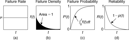
Figure 12-1. Typical plots of (a) the failure rate μ, (b) the failure density f(t), (c) the failure probability P(t), and (d) the reliability R(t).
Equations 12-1 through 12-5 are valid only for a constant failure rate μ. Many components exhibit a typical bathtub failure rate, shown in Figure 12-2. The failure rate is highest when the component is new (infant mortality) and when it is old (old age). Between these two periods (denoted by the lines in Figure 12-2), the failure rate is reasonably constant and Equations 12-1 through 12-5 are valid.
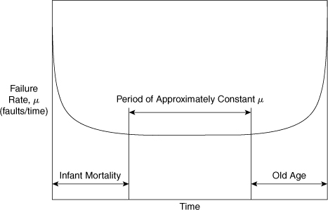
Figure 12-2. A typical bathtub failure rate curve for process hardware. The failure rate is approximately constant over the midlife of the component.
Interactions between Process Units
Accidents in chemical plants are usually the result of a complicated interaction of a number of process components. The overall process failure probability is computed from the individual component probabilities.
Process components interact in two different fashions. In some cases a process failure requires the simultaneous failure of a number of components in parallel. This parallel structure is represented by the logical AND function. This means that the failure probabilities for the individual components must be multiplied:
where
n is the total number of components and
Pi is the failure probability of each component.
This rule is easily memorized because for parallel components the probabilities are multiplied.
The total reliability for parallel units is given by
where Ri is the reliability of an individual process component.
Process components also interact in series. This means that a failure of any single component in the series of components will result in failure of the process. The logical OR function represents this case. For series components the overall process reliability is found by multiplying the reliabilities for the individual components:
The overall failure probability is computed from
For a system composed of two components A and B, Equation 12-9 is expanded to
The cross-product term P(A)P(B) compensates for counting the overlapping cases twice. Consider the example of tossing a single die and determining the probability that the number of points is even or divisible by 3. In this case
P(even or divisible by 3) = P(even) + P(divisible by 3) – P(even and divisible by 3).
The last term subtracts the cases in which both conditions are satisfied.
If the failure probabilities are small (a common situation), the term P(A)P(B) is negligible, and Equation 12-10 reduces to
This result is generalized for any number of components. For this special case Equation 12-9 reduces to
Failure rate data for a number of typical process components are provided in Table 12-1. These are average values determined at a typical chemical process facility. Actual values would depend on the manufacturer, materials of construction, the design, the environment, and other factors. The assumptions in this analysis are that the failures are independent, hard, and not intermittent and that the failure of one device does not stress adjacent devices to the point that the failure probability is increased.
Table 12-1. Failure Rate Data for Various Selected Process Componentsa
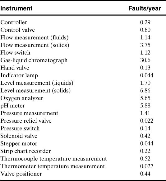
a Selected from Frank P. Lees, Loss Prevention in the Process Industries (London: Butterworths, 1986), p. 343.
A summary of computations for parallel and series process components is shown in Figure 12-3.
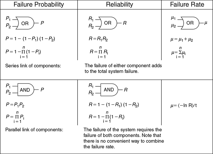
Figure 12-3. Computations for various types of component linkages.
The water flow to a chemical reactor cooling coil is controlled by the system shown in Figure 12-4. The flow is measured by a differential pressure (DP) device, the controller decides on an appropriate control strategy, and the control valve manipulates the flow of coolant. Determine the overall failure rate, the unreliability, the reliability, and the MTBF for this system. Assume a 1-yr period of operation.
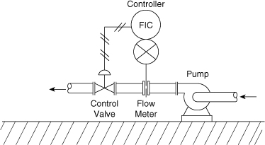
Figure 12-4. Flow control system. The components of the control system are linked in series.
These process components are related in series. Thus, if any one of the components fails, the entire system fails. The reliability and failure probability are computed for each component using Equations 12-1 and 12-2. The results are shown in the following table. The failure rates are from Table 12-1.
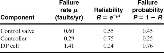
The overall reliability for components in series is computed using Equation 12-8. The result is
The failure probability is computed from
P = 1 – R = 1 – 0.10 = 0.90/yr.
The overall failure rate is computed using the definition of the reliability (Equation 12-1):
0.10 = e–μ
μ = –ln(0.10) = 2.30 failures/yr.
The MTBF is computed using Equation 12-5:
This system is expected to fail, on average, once every 0.43 yr.
A diagram of the safety systems in a certain chemical reactor is shown in Figure 12-5. This reactor contains a high-pressure alarm to alert the operator in the event of dangerous reactor pressures. It consists of a pressure switch within the reactor connected to an alarm light indicator. For additional safety an automatic high-pressure reactor shutdown system is installed. This system is activated at a pressure somewhat higher than the alarm system and consists of a pressure switch connected to a solenoid valve in the reactor feed line. The automatic system stops the flow of reactant in the event of dangerous pressures. Compute the overall failure rate, the failure probability, the reliability, and the MTBF for a high-pressure condition. Assume a 1-yr period of operation. Also, develop an expression for the overall failure probability based on the component failure probabilities.
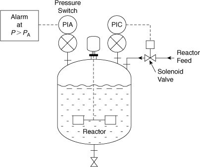
Figure 12-5. A chemical reactor with an alarm and an inlet feed solenoid. The alarm and feed shutdown systems are linked in parallel.
Failure rate data are available from Table 12-1. The reliability and failure probabilities of each component are computed using Equations 12-1 and 12-2:
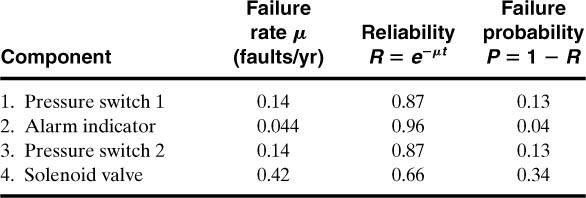
A dangerous high-pressure reactor situation occurs only when both the alarm system and the shutdown system fail. These two components are in parallel. For the alarm system the components are in series:
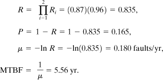
For the shutdown system the components are also in series:
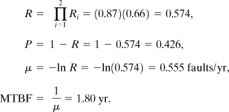
The two systems are combined using Equation 12-6:
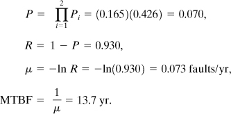
For the alarm system alone a failure is expected once every 5.5 yr. Similarly, for a reactor with a high-pressure shutdown system alone, a failure is expected once every 1.80 yr. However, with both systems in parallel the MTBF is significantly improved and a combined failure is expected every 13.7 yr.
The overall failure probability is given by
P = P(A)P(S),
where P(A) is the failure probability of the alarm system and P(S) is the failure probability of the emergency shutdown system. An alternative procedure is to invoke Equation 12-9 directly. For the alarm system
P(A) = P1 + P2 – P1P2.
P(S) = P3 + P4 – P3P4.
The overall failure probability is then
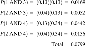
P = P(A)P(S) = (P1 + P2 – P1P2)(P3 + P4 – P3P4).
Substituting the numbers provided in the example, we obtain
P = [0.13 + 0.04 – (0.13)(0.04)][0.34 + 0.13 – (0.34)(0.13)]
= (0.165)(0.426) = 0.070.
This is the same answer as before.
If the products P1P2 and P3P4 are assumed to be small, then
P(A) = P1 + P2,
P(S) = P3 + P4,
and
P = P(A)P(S) = (P1 + P2)(P3 + P4)
= 0.080.
The difference between this answer and the answer obtained previously is 14.3%. The component probabilities are not small enough in this example to assume that the cross-products are negligible.
Revealed and Unrevealed Failures
Example 12-2 assumes that all failures in either the alarm or the shutdown system are immediately obvious to the operator and are fixed in a negligible amount of time. Emergency alarms and shutdown systems are used only when a dangerous situation occurs. It is possible for the equipment to fail without the operator being aware of the situation. This is called an unrevealed failure. Without regular and reliable equipment testing, alarm and emergency systems can fail without notice. Failures that are immediately obvious are called revealed failures.
A flat tire on a car is immediately obvious to the driver. However, the spare tire in the trunk might also be flat without the driver being aware of the problem until the spare is needed.
Figure 12-6 shows the nomenclature for revealed failures. The time that the component is operational is called the period of operation and is denoted by τo. After a failure occurs, a period of time, called the period of inactivity or downtime (τr), is required to repair the component. The MTBF is the sum of the period of operation and the downtime, as shown.
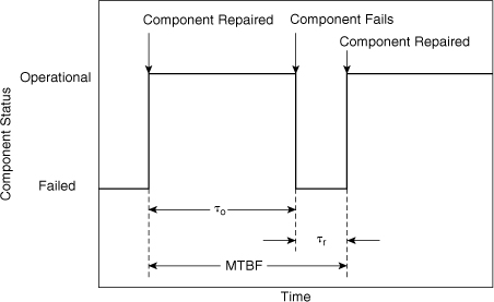
Figure 12-6. Component cycles for revealed failures. A failure requires a period of time for repair.
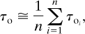
For revealed failures the period of inactivity or downtime for a particular component is computed by averaging the inactive period for a number of failures:
where
n is the number of times the failure or inactivity occurred and
τri is the period for repair for a particular failure.
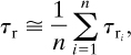
Similarly, the time before failure or period of operation is given by
where τoi is the period of operation between a particular set of failures.
The MTBF is the sum of the period of operation and the repair period:
It is convenient to define an availability and unavailability. The availability A is simply the probability that the component or process is found functioning. The unavailability U is the probability that the component or process is found not functioning. It is obvious that
The quantity τo represents the period that the process is in operation, and τr + τo represents the total time. By definition, it follows that the availability is given by
and, similarly, the unavailability is
By combining Equations 12-16 and 12-17 with the result of Equation 12-14, we can write the equations for the availability and unavailability for revealed failures:

For unrevealed failures the failure becomes obvious only after regular inspection. This situation is shown in Figure 12-7. If τu is the average period of unavailability during the inspection interval and if τi is the inspection interval, then
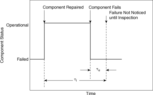
Figure 12-7. Component cycles for unrevealed failures.
The average period of unavailability is computed from the failure probability:
Combining with Equation 12-19, we obtain
The failure probability P(t) is given by Equation 12-2. This is substituted into Equation 12-21 and integrated. The result is
An expression for the availability is
If the term μτi ![]() 1, then the failure probability is approximated by
1, then the failure probability is approximated by
and Equation 12-21 is integrated to give, for unrevealed failures,

This is a useful and convenient result. It demonstrates that, on average, for unrevealed failures the process or component is unavailable during a period equal to half the inspection interval. A decrease in the inspection interval is shown to increase the availability of an unrevealed failure.
Equations 12-19 through 12-25 assume a negligible repair time. This is usually a valid assumption because on-line process equipment is generally repaired within hours, whereas the inspection intervals are usually monthly.
Compute the availability and the unavailability for both the alarm and the shutdown systems of Example 12-2. Assume that a maintenance inspection occurs once every month and that the repair time is negligible.
Both systems demonstrate unrevealed failures. For the alarm system the failure rate is μ = 0.18 faults/yr. The inspection period is 1/12 = 0.083 yr. The unavailability is computed using Equation 12-25:
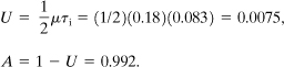
The alarm system is available 99.2% of the time. For the shutdown system μ = 0.55 faults/yr. Thus
The shutdown system is available 97.7% of the time.
Probability of Coincidence
All process components demonstrate unavailability as a result of a failure. For alarms and emergency systems it is unlikely that these systems will be unavailable when a dangerous process episode occurs. The danger results only when a process upset occurs and the emergency system is unavailable. This requires a coincidence of events.
Assume that a dangerous process episode occurs pd times in a time interval Ti. The frequency of this episode is given by
For an emergency system with unavailability U, a dangerous situation will occur only when the process episode occurs and the emergency system is unavailable. This is every pdU episodes.
The average frequency of dangerous episodes λd is the number of dangerous coincidences divided by the time period:
For small failure rates ![]() and pd = λTi. Substituting into Equation 12-27 yields
and pd = λTi. Substituting into Equation 12-27 yields
The mean time between coincidences (MTBC) is the reciprocal of the average frequency of dangerous coincidences:
For the reactor of Example 12-3 a high-pressure incident is expected once every 14 months. Compute the MTBC for a high-pressure excursion and a failure in the emergency shutdown device. Assume that a maintenance inspection occurs every month.
The frequency of process episodes is given by Equation 12-26:
λ = 1 episode/[(14 months)(1 yr/12 months)] = 0.857/yr.
The unavailability is computed from Equation 12-25:
The average frequency of dangerous coincidences is given by Equation 12-27:
λd = λU = (0.857)(0.023) = 0.020.
The MTBC is (from Equation 12-29)
It is expected that a simultaneous high-pressure incident and failure of the emergency shutdown device will occur once every 50 yr.
If the inspection interval τi is halved, then U = 0.023, λd = 0.010, and the resulting MTBC is 100 yr. This is a significant improvement and shows why a proper and timely maintenance program is important.
Redundancy2
Systems are designed to function normally even when a single instrument or control function fails. This is achieved with redundant controls, including two or more measurements, processing paths, and actuators that ensure that the system operates safely and reliably. The degree of redundancy depends on the hazards of the process and on the potential for economic losses. An example of a redundant temperature measurement is an additional temperature probe. An example of a redundant temperature control loop is an additional temperature probe, controller, and actuator (for example, cooling water control valve).
Common Mode Failures
Occasionally an incident occurs that results in a common mode failure. This is a single event that affects a number of pieces of hardware simultaneously. For example, consider several flow control loops similar to Figure 12-4. A common mode failure is the loss of electrical power or a loss of instrument air. A utility failure of this type can cause all the control loops to fail at the same time. The utility is connected to these systems via OR gates. This increases the failure rate substantially. When working with control systems, one needs to deliberately design the systems to minimize common cause failures.
12-2. Event Trees
Event trees begin with an initiating event and work toward a final result. This approach is inductive. The method provides information on how a failure can occur and the probability of occurrence.
When an accident occurs in a plant, various safety systems come into play to prevent the accident from propagating. These safety systems either fail or succeed. The event tree approach includes the effects of an event initiation followed by the impact of the safety systems.
The typical steps in an event tree analysis are3
1. Identify an initiating event of interest,
2. Identify the safety functions designed to deal with the initiating event,
3. Construct the event tree, and
4. Describe the resulting accident event sequences.
If appropriate data are available, the procedure is used to assign numerical values to the various events. This is used effectively to determine the probability of a certain sequence of events and to decide what improvements are required.
Consider the chemical reactor system shown in Figure 12-8. A high-temperature alarm has been installed to warn the operator of a high temperature within the reactor. The event tree for a loss-of-coolant initiating event is shown in Figure 12-9. Four safety functions are identified. These are written across the top of the sheet. The first safety function is the high-temperature alarm. The second safety function is the operator noticing the high reactor temperature during normal inspection. The third safety function is the operator reestablishing the coolant flow by correcting the problem in time. The final safety function is invoked by the operator performing an emergency shutdown of the reactor. These safety functions are written across the page in the order in which they logically occur.
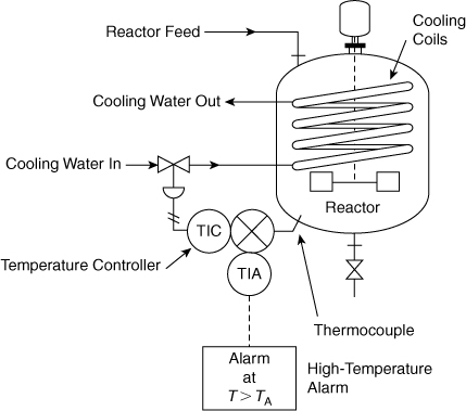
Figure 12-8. Reactor with high-temperature alarm and temperature controller.
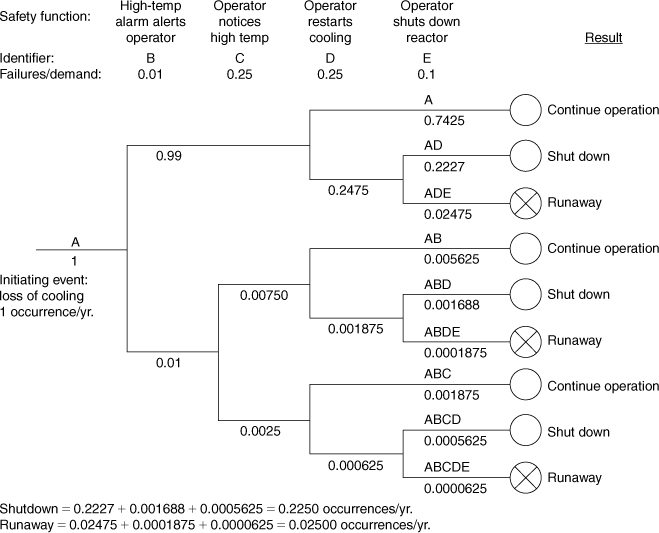
Figure 12-9. Event tree for a loss-of-coolant accident for the reactor of Figure 12-8.
The event tree is written from left to right. The initiating event is written first in the center of the page on the left. A line is drawn from the initiating event to the first safety function. At this point the safety function can either succeed or fail. By convention, a successful operation is drawn by a straight line upward and a failure is drawn downward. Horizontal lines are drawn from these two states to the next safety function.
If a safety function does not apply, the horizontal line is continued through the safety function without branching. For this example, the upper branch continues through the second function, where the operator notices the high temperature. If the high-temperature alarm operates properly, the operator will already be aware of the high-temperature condition. The sequence description and consequences are indicated on the extreme right-hand side of the event tree. The open circles indicate safe conditions, and the circles with the crosses represent unsafe conditions.
The lettering notation in the sequence description column is useful for identifying the particular event. The letters indicate the sequence of failures of the safety systems. The initiating event is always included as the first letter in the notation. An event tree for a different initiating event in this study would use a different letter. For the example here, the lettering sequence ADE represents initiating event A followed by failure of safety functions D and E.
The event tree can be used quantitatively if data are available on the failure rates of the safety functions and the occurrence rate of the initiation event. For this example assume that a loss-of-cooling event occurs once a year. Let us also assume that the hardware safety functions fail 1% of the time they are placed in demand. This is a failure rate of 0.01 failure/demand. Also assume that the operator will notice the high reactor temperature 3 out of 4 times and that 3 out of 4 times the operator will be successful at reestablishing the coolant flow. Both of these cases represent a failure rate of 1 time out of 4, or 0.25 failure/demand. Finally, it is estimated that the operator successfully shuts down the system 9 out of 10 times. This is a failure rate of 0.10 failure/demand.
The failure rates for the safety functions are written below the column headings. The occurrence frequency for the initiating event is written below the line originating from the initiating event.
The computational sequence performed at each junction is shown in Figure 12-10. Again, the upper branch, by convention, represents a successful safety function and the lower branch represents a failure. The frequency associated with the lower branch is computed by multiplying the failure rate of the safety function times the frequency of the incoming branch. The frequency associated with the upper branch is computed by subtracting the failure rate of the safety function from 1 (giving the success rate of the safety function) and then multiplying by the frequency of the incoming branch.
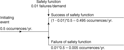
Figure 12-10. The computational sequence across a safety function in an event tree.
The net frequency associated with the event tree shown in Figure 12-9 is the sum of the frequencies of the unsafe states (the states with the circles and x’s). For this example the net frequency is estimated at 0.025 failure per year (sum of failures ADE, ABDE, and ABCDE).
This event tree analysis shows that a dangerous runaway reaction will occur on average 0.025 time per year, or once every 40 years. This is considered too high for this installation. A possible solution is the inclusion of a high-temperature reactor shutdown system. This control system would automatically shut down the reactor in the event that the reactor temperature exceeds a fixed value. The emergency shutdown temperature would be higher than the alarm value to provide an opportunity for the operator to restore the coolant flow.
The event tree for the modified process is shown in Figure 12-11. The additional safety function provides a backup in the event that the high-temperature alarm fails or the operator fails to notice the high temperature. The runaway reaction is now estimated to occur 0.00025 time per year, or once every 400 years. This is a substantial improvement obtained by the addition of a simple redundant shutdown system.
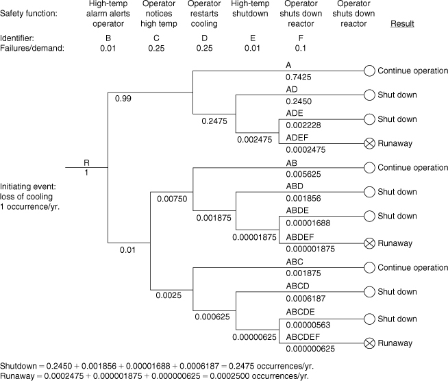
Figure 12-11. Event tree for the reactor of Figure 12-8. This includes a high-temperature shutdown system.
The event tree is useful for providing scenarios of possible failure modes. If quantitative data are available, an estimate can be made of the failure frequency. This is used most successfully to modify the design to improve the safety. The difficulty is that for most real processes the method can be extremely detailed, resulting in a huge event tree. If a probabilistic computation is attempted, data must be available for every safety function in the event tree.
An event tree begins with a specified failure and terminates with a number of resulting consequences. If an engineer is concerned about a particular consequence, there is no certainty that the consequence of interest will actually result from the selected failure. This is perhaps the major disadvantage of event trees.
12-3. Fault Trees
Fault trees originated in the aerospace industry and have been used extensively by the nuclear power industry to qualify and quantify the hazards and risks associated with nuclear power plants. This approach is becoming more popular in the chemical process industries, mostly as a result of the successful experiences demonstrated by the nuclear industry.
A fault tree for anything but the simplest of plants can be large, involving thousands of process events. Fortunately, this approach lends itself to computerization, with a variety of computer programs commercially available to draw fault trees based on an interactive session.
Fault trees are a deductive method for identifying ways in which hazards can lead to accidents. The approach starts with a well-defined accident, or top event, and works backward toward the various scenarios that can cause the accident.
For instance, a flat tire on an automobile is caused by two possible events. In one case the flat is due to driving over debris on the road, such as a nail. The other possible cause is tire failure. The flat tire is identified as the top event. The two contributing causes are either basic or intermediate events. The basic events are events that cannot be defined further, and intermediate events are events that can. For this example, driving over the road debris is a basic event because no further definition is possible. The tire failure is an intermediate event because it results from either a defective tire or a worn tire.
The flat tire example is pictured using a fault tree logic diagram, shown in Figure 12-12. The circles denote basic events and the rectangles denote intermediate events. The fishlike symbol represents the OR logic function. It means that either of the input events will cause the output state to occur. As shown in Figure 12-12, the flat tire is caused by either debris on the road or tire failure. Similarly, the tire failure is caused by either a defective tire or a worn tire.
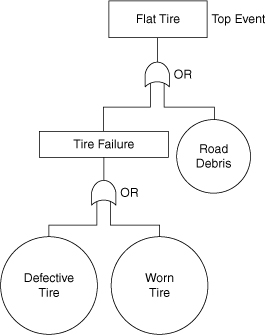
Figure 12-12. A fault tree describing the various events contributing to a flat tire.
Events in a fault tree are not restricted to hardware failures. They can also include software, human, and environmental factors.
For reasonably complex chemical processes a number of additional logic functions are needed to construct a fault tree. A detailed list is given in Figure 12-13. The AND logic function is important for describing processes that interact in parallel. This means that the output state of the AND logic function is active only when both of the input states are active. The INHIBIT function is useful for events that lead to a failure only part of the time. For instance, driving over debris in the road does not always lead to a flat tire. The INHIBIT gate could be used in the fault tree of Figure 12-12 to represent this situation.
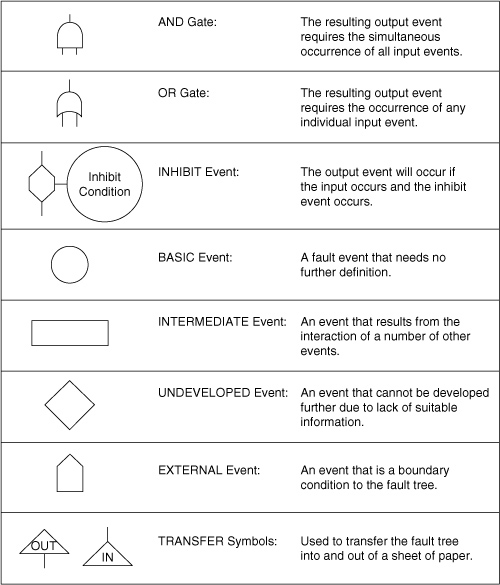
Figure 12-13. The logic transfer components used in a fault tree.
Before the actual fault tree is drawn, a number of preliminary steps must be taken:
1. Define precisely the top event. Events such as “high reactor temperature” or “liquid level too high” are precise and appropriate. Events such as “explosion of reactor” or “fire in process” are too vague, whereas an event such as “leak in valve” is too specific.
2. Define the existing event. What conditions are sure to be present when the top event occurs?
3. Define the unallowed events. These are events that are unlikely or are not under consideration at the present. This could include wiring failures, lightning, tornadoes, and hurricanes.
4. Define the physical bounds of the process. What components are to be considered in the fault tree?
5. Define the equipment configuration. What valves are open or closed? What are the liquid levels? Is this a normal operation state?
6. Define the level of resolution. Will the analysis consider just a valve, or will it be necessary to consider the valve components?
The next step in the procedure is to draw the fault tree. First, draw the top event at the top of the page. Label it as the top event to avoid confusion later when the fault tree has spread out to several sheets of paper.
Second, determine the major events that contribute to the top event. Write these down as intermediate, basic, undeveloped, or external events on the sheet. If these events are related in parallel (all events must occur in order for the top event to occur), they must be connected to the top event by an AND gate. If these events are related in series (any event can occur in order for the top event to occur), they must be connected by an OR gate. If the new events cannot be related to the top event by a single logic function, the new events are probably improperly specified. Remember, the purpose of the fault tree is to determine the individual event steps that must occur to produce the top event.
Now consider any one of the new intermediate events. What events must occur to contribute to this single event? Write these down as either intermediate, basic, undeveloped, or external events on the tree. Then decide which logic function represents the interaction of these newest events.
Continue developing the fault tree until all branches have been terminated by basic, undeveloped, or external events. All intermediate events must be expanded.
Consider again the alarm indicator and emergency shutdown system of Example 12-5. Draw a fault tree for this system.
The first step is to define the problem.
1. Top event: Damage to reactor as a result of overpressuring.
2. Existing event: High process pressure.
3. Unallowed events: Failure of mixer, electrical failures, wiring failures, tornadoes, hurricanes, electrical storms.
4. Physical bounds: The equipment shown in Figure 12-5.
5. Equipment configuration: Solenoid valve open, reactor feed flowing.
6. Level of resolution: Equipment as shown in Figure 12-5.
The top event is written at the top of the fault tree and is indicated as the top event (see Figure 12-14). Two events must occur for overpressuring: failure of the alarm indicator and failure of the emergency shutdown system. These events must occur together so they must be connected by an AND function. The alarm indicator can fail by a failure of either pressure switch 1 or the alarm indicator light. These must be connected by OR functions. The emergency shutdown system can fail by a failure of either pressure switch 2 or the solenoid valve. These must also be connected by an OR function. The complete fault tree is shown in Figure 12-14.
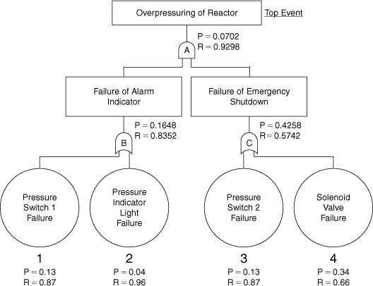
Figure 12-14. Fault tree for Example 12-5.
Determining the Minimal Cut Sets
Once the fault tree has been fully drawn, a number of computations can be performed. The first computation determines the minimal cut sets (or min cut sets). The minimal cut sets are the various sets of events that could lead to the top event. In general, the top event could occur through a variety of different combinations of events. The different unique sets of events leading to the top event are the minimal cut sets.
The minimal cut sets are useful for determining the various ways in which a top event could occur. Some of the mimimal cut sets have a higher probability than others. For instance, a set involving just two events is more likely than a set involving three. Similarly, a set involving human interaction is more likely to fail than one involving hardware alone. Based on these simple rules, the minimal cut sets are ordered with respect to failure probability. The higher probability sets are examined carefully to determine whether additional safety systems are required.
The minimal cut sets are determined using a procedure developed by Fussell and Vesely.4 The procedure is best described using an example.
Determine the minimal cut sets for the fault tree of Example 12-5.
The first step in the procedure is to label all the gates using letters and to label all the basic events using numbers. This is shown in Figure 12-14. The first logic gate below the top event is written:
A
AND gates increase the number of events in the cut sets, whereas OR gates lead to more sets. Logic gate A in Figure 12-14 has two inputs: one from gate B and the other from gate C. Because gate A is an AND gate, gate A is replaced by gates B and C:
Gate B has inputs from event 1 and event 2. Because gate B is an OR gate, gate B is replaced by adding an additional row below the present row. First, replace gate B by one of the inputs, and then create a second row below the first. Copy into this new row all the entries in the remaining column of the first row:
Note that the C in the second column of the first row is copied to the new row.
Next, replace gate C in the first row by its inputs. Because gate C is also an OR gate, replace C by basic event 3 and then create a third row with the other event. Be sure to copy the 1 from the other column of the first row:

Finally, replace gate C in the second row by its inputs. This generates a fourth row:

The cut sets are then
1, 3
2, 3
1, 4
2, 4
This means that the top event occurs as a result of any one of these sets of basic events.
The procedure does not always deliver the minimal cut sets. Sometimes a set might be of the following form:
1, 2, 2
This is reduced to simply 1, 2. On other occasions the sets might include supersets. For instance, consider
1, 2
1, 2, 4
1, 2, 3
The second and third sets are supersets of the first basic set because events 1 and 2 are in common.
The supersets are eliminated to produce the minimal cut sets.
For this example there are no supersets.
Quantitative Calculations Using the Fault Tree
The fault tree can be used to perform quantitative calculations to determine the probability of the top event. This is accomplished in two ways.
With the first approach the computations are performed using the fault tree diagram itself. The failure probabilities of all the basic, external, and undeveloped events are written on the fault tree. Then the necessary computations are performed across the various logic gates. Remember that probabilities are multiplied across an AND gate and that reliabilities are multiplied across an OR gate. The computations are continued in this fashion until the top event is reached. INHIBIT gates are considered a special case of an AND gate.
The results of this procedure are shown in Figure 12-14. The symbol P represents the probability and R represents the reliability. The failure probabilities for the basic events were obtained from Example 12-2.
The other procedure is to use the minimal cut sets. This procedure approaches the exact result only if the probabilities of all the events are small. In general, this result provides a number that is larger than the actual probability. This approach assumes that the probability cross-product terms shown in Equation 12-10 are negligible.
The minimal cut sets represent the various failure modes. For Example 12-6 events 1, 3 or 2, 3 or 1, 4 or 2, 4 could cause the top event. To estimate the overall failure probability, the probabilities from the cut sets are added together. For this case
This compares to the exact result of 0.0702 obtained using the actual fault tree. The cut sets are related to each other by the OR function. For Example 12-6 all the cut set probabilities were added. This is an approximate result, as shown by Equation 12-10, because the cross-product terms were neglected. For small probabilities the cross-product terms are negligible and the addition will approach the true result.
Advantages and Disadvantages of Fault Trees
The main disadvantage of using fault trees is that for any reasonably complicated process the fault tree will be enormous. Fault trees involving thousands of gates and intermediate events are not unusual. Fault trees of this size require a considerable amount of time, measured in years, to complete.
Furthermore, the developer of a fault tree can never be certain that all the failure modes have been considered. More complete fault trees are usually developed by more experienced engineers.
Fault trees also assume that failures are “hard,” that a particular item of hardware does not fail partially. A leaking valve is a good example of a partial failure. Also, the approach assumes that a failure of one component does not stress the other components, resulting in a change in the component failure probabilities.
Fault trees developed by different individuals are usually different in structure. The different trees generally predict different failure probabilities. This inexact nature of fault trees is a considerable problem.
If the fault tree is used to compute a failure probability for the top event, then failure probabilities are needed for all the events in the fault tree. These probabilities are not usually known or are not known accurately.
A major advantage of the fault tree approach is that it begins with a top event. This top event is selected by the user to be specific to the failure of interest. This is opposed to the event tree approach, where the events resulting from a single failure might not be the events of specific interest to the user.
Fault trees are also used to determine the minimal cut sets. The minimal cut sets provide enormous insight into the various ways for top events to occur. Some companies adopt a control strategy to have all their minimal cut sets be a product of four or more independent failures. This, of course, increases the reliability of the system significantly.
Finally, the entire fault tree procedure enables the application of computers. Software is available for graphically constructing fault trees, determining the minimal cut sets, and calculating failure probabilities. Reference libraries containing failure probabilities for various types of process equipment can also be included.
Relationship between Fault Trees and Event Trees
Event trees begin with an initiating event and work toward the top event (induction). Fault trees begin with a top event and work backward toward the initiating event (deduction).
The initiating events are the causes of the incident, and the top events are the final outcomes. The two methods are related in that the top events for fault trees are the initiating events for the event trees. Both are used together to produce a complete picture of an incident, from its initiating causes all the way to its final outcome. Probabilities and frequencies are attached to these diagrams.
12-4. QRA and LOPA
Risk is the product of the probability of a release, the probability of exposure, and the consequences of the exposure. Risk is usually described graphically, as shown in Figure 12-15. All companies decide their levels of acceptable risk and unacceptable risk. The actual risk of a process or plant is usually determined using quantitative risk analysis (QRA) or a layer of protection analysis (LOPA). Other methods are sometimes used; however, QRA and LOPA are the methods that are most commonly used. In both methods the frequency of the release is determined using a combination of event trees, fault trees, or an appropriate adaptation.
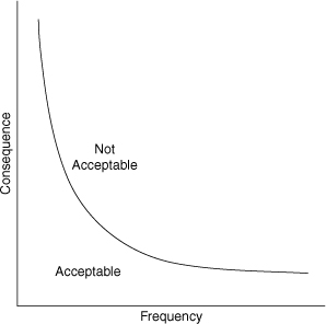
Figure 12-15. General description of risk.
Quantitative Risk Analysis5
QRA is a method that identifies where operations, engineering, or management systems can be modified to reduce risk. The complexity of a QRA depends on the objectives of the study and the available information. Maximum benefits result when QRAs are used at the beginning of a project (conceptual review and design phases) and are maintained throughout the facility’s life cycle.
The QRA method is designed to provide managers with a tool to help them evaluate the overall risk of a process. QRAs are used to evaluate potential risks when qualitative methods cannot provide an adequate understanding of the risks. QRA is especially effective for evaluating alternative risk reduction strategies.
The major steps of a QRA study include
1. Defining the potential event sequences and potential incidents,
2. Evaluating the incident consequences (the typical tools for this step include dispersion modeling and fire and explosion modeling),
3. Estimating the potential incident frequencies using event trees and fault trees,
4. Estimating the incident impacts on people, environment, and property, and
5. Estimating the risk by combining the impacts and frequencies, and recording the risk using a graph similar to Figure 12-15.
In general, QRA is a relatively complex procedure that requires expertise and a substantial commitment of resources and time. In some instances this complexity may not be warranted; then the application of LOPA methods may be more appropriate.
Layer of Protection Analysis6
LOPA is a semi-quantitative tool for analyzing and assessing risk. This method includes simplified methods to characterize the consequences and estimate the frequencies. Various layers of protection are added to a process, for example, to lower the frequency of the undesired consequences. The protection layers may include inherently safer concepts; the basic process control system; safety instrumented functions; passive devices, such as dikes or blast walls; active devices, such as relief valves; and human intervention. This concept of layers of protection is illustrated in Figure 12-16. The combined effects of the protection layers and the consequences are then compared against some risk tolerance criteria.
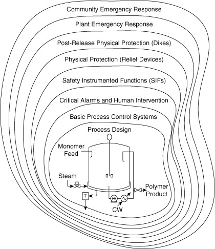
Figure 12-16. Layers of protection to lower the frequency of a specific accident scenario.
In LOPA the consequences and effects are approximated by categories, the frequencies are estimated, and the effectiveness of the protection layers is also approximated. The approximate values and categories are selected to provide conservative results. Thus the results of a LOPA should always be more conservative than those from a QRA. If the LOPA results are unsatisfactory or if there is any uncertainty in the results, then a full QRA may be justified. The results of both methods need to be used cautiously. However, the results of QRA and LOPA studies are especially satisfactory when comparing alternatives.
Individual companies use different criteria to establish the boundary between acceptable and unacceptable risk. The criteria may include frequency of fatalities, frequency of fires, maximum frequency of a specific category of a consequence, and required number of independent layers of protection for a specific consequence category.
The primary purpose of LOPA is to determine whether there are sufficient layers of protection against a specific accident scenario. As illustrated in Figure 12-16, many types of protective layers are possible. Figure 12-16 does not include all possible layers of protection. A scenario may require one or many layers of protection, depending on the process complexity and potential severity of an accident. Note that for a given scenario only one layer must work successfully for the consequence to be prevented. Because no layer is perfectly effective, however, sufficient layers must be added to the process to reduce the risk to an acceptable level.
The major steps of a LOPA study include
1. Identifying a single consequence (a simple method to determine consequence categories is described later)
2. Identifying an accident scenario and cause associated with the consequence (the scenario consists of a single cause-consequence pair)
3. Identifying the initiating event for the scenario and estimating the initiating event frequency (a simple method is described later)
4. Identifying the protection layers available for this particular consequence and estimating the probability of failure on demand for each protection layer
5. Combining the initiating event frequency with the probabilities of failure on demand for the independent protection layers to estimate a mitigated consequence frequency for this initiating event
6. Plotting the consequence versus the consequence frequency to estimate the risk (the risk is usually shown in a figure similar to Figure 12-15)
7. Evaluating the risk for acceptability (if unacceptable, additional layers of protection are required)
This procedure is repeated for other consequences and scenarios. A number of variations on this procedure are used.
Consequence
The most common scenario of interest for LOPA in the chemical process industry is loss of containment of hazardous material. This can occur through a variety of incidents, such as a leak from a vessel, a ruptured pipeline, a gasket failure, or release from a relief valve.
In a QRA study the consequences of these releases are quantified using dispersion modeling and a detailed analysis to determine the downwind consequences as a result of fires, explosions, or toxicity. In a LOPA study the consequences are estimated using one of the following methods: (1) semi-quantitative approach without the direct reference to human harm, (2) qualitative estimates with human harm, and (3) quantitative estimates with human harm. See the reference mentioned in footnote 6 for the detailed methods.
When using the semi-quantitative method, the quantity of the release is estimated using source models, and the consequences are characterized with a category, as shown in Table 12-2. This is an easy method to use compared with QRA.
Table 12-2. Semi-Quantitative Consequences Categorization
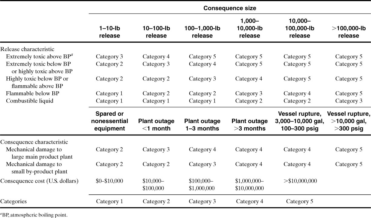
Although the method is easy to use, it clearly identifies problems that may need additional work, such as a QRA. It also identifies problems that may be deemphasized because the consequences are insignificant.
Frequency
When conducting a LOPA study, several methods can be used to determine the frequency. One of the less rigorous methods includes the following steps:
1. Determine the failure frequency of the initiating event.
2. Adjust this frequency to include the demand; for example, a reactor failure frequency is divided by 12 if the reactor is used only 1 month during the entire year. The frequencies are also adjusted (reduced) to include the benefits of preventive maintenance. If, for example, a control system is given preventive maintenance 4 times each year, then its failure frequency is divided by 4.
3. Adjust the failure frequency to include the probabilities of failure on demand (PFDs) for each independent layer of protection.
The failure frequencies for the common initiating events of an accident scenario are shown in Table 12-3.
Table 12-3. Typical Frequency Values Assigned to Initiating Eventsa
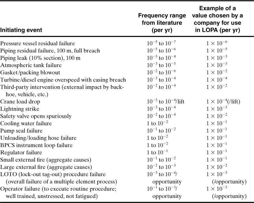
a Individual companies choose their own values, consistent with the degree of conservatism or the company’s risk tolerance criteria. Failure rates can also be greatly affected by preventive maintenance routines.
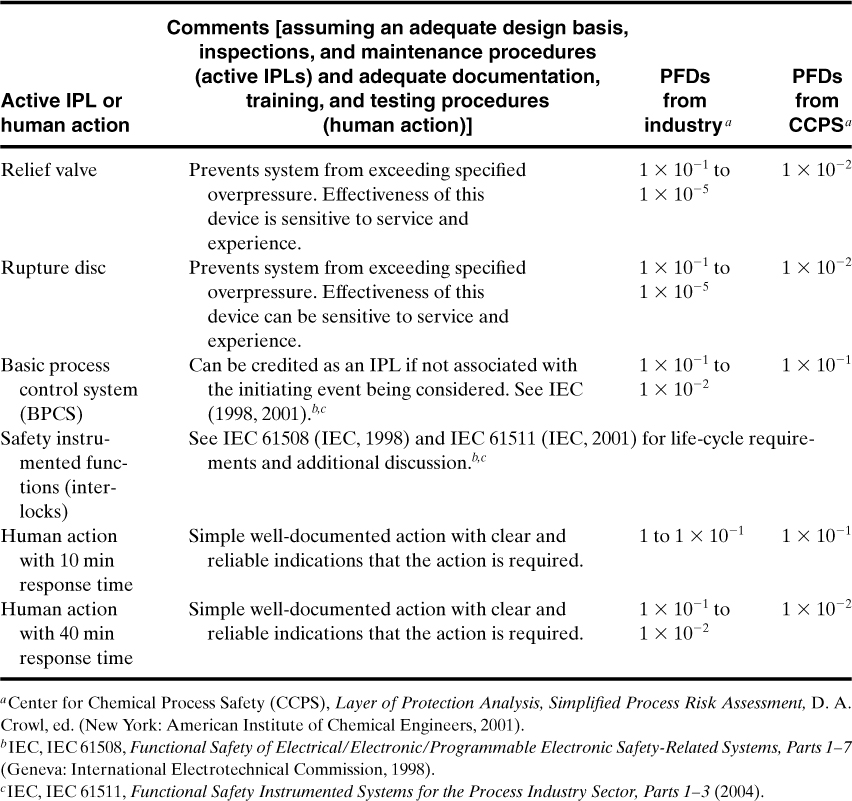
The PFD for each independent protection layer (IPL) varies from 10–1 to 10–5 for a weak IPL and a strong IPL, respectively. The common practice is to use a PFD of 10–2 unless experience shows it to be higher or lower. Some PFDs recommended by CCPS (see footnote 6) for screening are given in Tables 12-4 and 12-5. There are three rules for classifying a specific system or action of an IPL:
1. The IPL is effective in preventing the consequence when it functions as designed.
2. The IPL functions independently of the initiating event and the components of all other IPLs that are used for the same scenario.
3. The IPL is auditable, that is, the PFD of the IPL must be capable of validation including review, testing, and documentation.
Table 12-4. PFDs for Passive IPLs
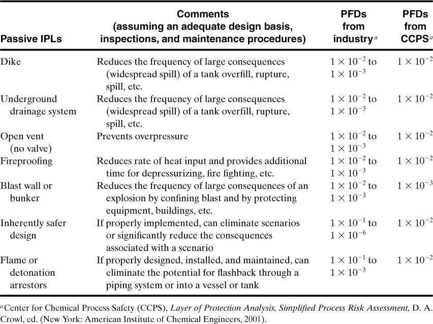
Table 12-5. PFDs for Active IPLs and Human Actions
The frequency of a consequence of a specific scenario endpoint is computed using
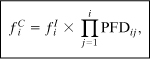
where
![]() is the mitigated consequence frequency for a specific consequence C for an initiating event i,
is the mitigated consequence frequency for a specific consequence C for an initiating event i,
![]() is the initiating event frequency for the initiating event i, and
is the initiating event frequency for the initiating event i, and
PFDij is the probability of failure of the jth IPL that protects against the specific consequence and the specific initiating event i. The PFD is usually 10–2, as described previously.
When there are multiple scenarios with the same consequence, each scenario is evaluated individually using Equation 12-30. The frequency of the consequence is subsequently determined using

![]() is the frequency of the Cth consequence for the ith initiating event and
is the frequency of the Cth consequence for the ith initiating event and
I is the total number of initiating events for the same consequence.
Determine the consequence frequency for a cooling water failure if the system is designed with two IPLs. The IPLs are human interaction with 10-min response time and a basic process control system (BPCS).
The frequency of a cooling water failure is taken from Table 12-3; that is, ![]() . The PFDs are estimated from Tables 12-4 and 12-5. The human response PFD is 10–1 and the PFD for the BPCS is 10–1. The consequence frequency is found using Equation 12-30:
. The PFDs are estimated from Tables 12-4 and 12-5. The human response PFD is 10–1 and the PFD for the BPCS is 10–1. The consequence frequency is found using Equation 12-30:
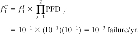
As illustrated in Example 12-7, the failure frequency is determined easily by using LOPA methods.
The concept of PFD is also used when designing emergency shutdown systems called safety instrumented functions (SIFs). A SIF achieves low PFD figures by
• Using redundant sensors and final redundant control elements
• Using multiple sensors with voting systems and redundant final control elements
• Testing the system components at specific intervals to reduce the probability of failures on demand by detecting hidden failures
• Using a deenergized trip system (i.e., a relayed shutdown system)
There are three safety integrity levels (SILs) that are generally accepted in the chemical process industry for emergency shutdown systems:
1. SIL1 (PFD = 10–1 to 10–2): These SIFs are normally implemented with a single sensor, a single logic solver, and a single final control element, and they require periodic proof testing.
2. SIL2 (PFD = 10–2 to 10–3): These SIFs are typically fully redundant, including the sensor, logic solver, and final control element, and they require periodic proof testing.
3. SIL3 (PFD = 10–3 to 10–4): SIL3 systems are typically fully redundant, including the sensor, logic solver, and final control element; and the system requires careful design and frequent validation tests to achieve the low PFD figures. Many companies find that they have a limited number of SIL3 systems because of the high cost normally associated with this architecture.
Typical LOPA
A typical LOPA study addresses about 2% to 5% of the significant issues defined in a PHA. To do this, each company develops limits for LOPA studies, for example, major consequences with a Category 4 and accidents with one or more fatalities. Effective LOPA studies should focus on areas that are associated with major accidents based on historical data, especially startups and shutdowns. It is generally accepted that 70% of accidents occur during startup and shutdown; therefore it is recommended that significant effort be devoted to these areas.7 Less time on LOPAs leaves more time for PHAs to identify other undiscovered and significant accident scenarios.
Each identified independent protection layer (IPL), or safeguard, is evaluated for two characteristics: (1) Is the IPL effective in preventing the scenario from reaching the consequences? and (2) Is the safeguard independent? All IPLs, in addition to being independent, have three characteristics:8
• Detect or sense the initiating event in the specific scenario
• Decide to take action or not
• Deflect and eliminate the undesired consequences
Some of the benefits of LOPAs are that they (1) focus attention on the major issues, (2) eliminate unnecessary safeguards, (3) establish valid safeguards to improve the PHA process, (4) require fewer resources and are faster than fault tree analysis or QRAs, and (5) provide a basis for managing layers of protection, such as spare parts and maintenance.
The general format for an LOPA is shown in Example 12-8.
A PHA team has identified several major consequences with different initiating events and frequencies. Develop a table to document the LOPA results for two of the major scenarios. The first scenario is for a fire due to a tank rupture, and the second scenario is for a release from a reactor because of a control loop failure. Both scenarios have a vessel volume of 50,000 lb of a flammable above the BP, and the failures result in a six-month outage. The reactor is operated 100 days in a year.
The LOPA results are shown in Table 12-6. A typical LOPA team develops a table with many columns for all significant events.
Table 12-6. General Format of LOPA
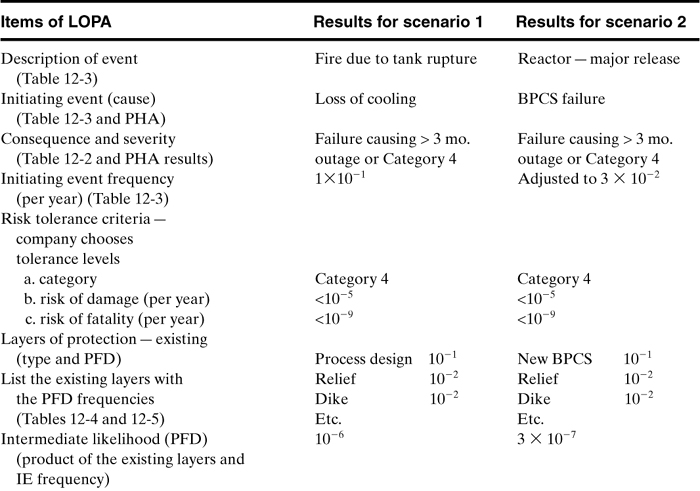
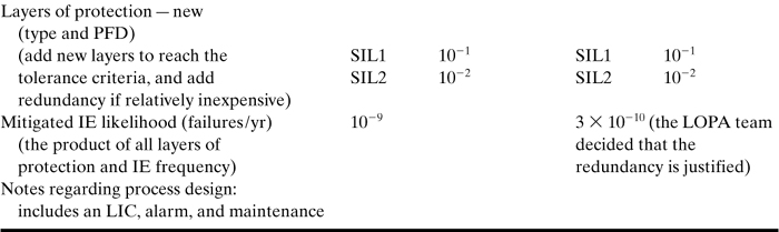
The batch reactor initiating event (IE) frequency is adjusted for the 100 days of operation; that is, the initiating frequency is 10-1 failures per year times 100/300 or a frequency of 3.0 × 10⁻².
As illustrated above, the resulting table contains information for characterizing risk (consequence and frequency). In each case the mitigated event frequencies are compared to the tolerable risk, and additional IPLs are added to reach these criteria. The results are an order of magnitude approximation of the risk, but the numbers in the tables give conservative estimates of failure probabilities. So the absolute risk may be off, but the comparisons of conservative risks identify the areas needing attention.
This method, therefore, identifies controls for reducing the frequency. However, the LOPA and PHA team members should also consider inherently safe design alternatives (see Section 1-7). Additional LOPA details, methods, examples, and references are in the CCPS books.9,10
Suggested Reading
Center for Chemical Process Safety (CCPS), Guidelines for Chemical Process Quantitative Risk Analysis 2nd ed. (New York: American Institute of Chemical Engineers 2000).
Center for Chemical Process Safety (CCPS), Guidelines for Consequence Analysis of Chemical Releases (New York: American Institute of Chemical Engineers, 1999).
Center for Chemical Process Safety (CCPS), Guidelines for Developing Quantitative Safety Risk Criteria (New York: American Institute of Chemical Engineers 2009).
Center for Chemical Process Safety (CCPS), Guidelines for Hazard Evaluation Procedures, 3rd ed. (New York: American Institute of Chemical Engineers, 2009).
Center for Chemical Process Safety (CCPS), Guidelines for Risk-Based Process Safety (New York: American Institute for Chemical Engineers, 2008).
Center for Chemical Process Safety (CCPS), Initiating Events and Independent Protection Layers for LOPA (New York: American Institute of Chemical Engineers, 2010).
Center for Chemical Process Safety (CCPS), Layer of Protection Analysis: Simplified Process Risk Assessment, D. A. Crowl, ed. (New York: American Institute of Chemical Engineers, 2001).
Arthur M. Dowell III, “Layer of Protection Analysis and Inherently Safer processes,” Process Safety Progress (1999), 18(4): 214–220.
Raymond Freeman, “Using Layer of Protection Analysis to Define Safety Integrity Level Requirements,” Process Safety Progress (Sept. 2007), 26(3): 185–194.
J. B. Fussell and W. E. Vesely, “A New Methodology for Obtaining Cut Sets for Fault Trees,” Transactions of the American Nuclear Society (1972), 15.
J. F. Louvar and B. D. Louvar, Health and Environmental Risk Analysis: Fundamentals with Applications (Upper Saddle River, NJ: Prentice Hall PTR, 1998).
S. Mannan, ed., Lees’ Loss Prevention in the Process Industries, 3rd ed. (London: Butterworth Heinemann, 2005).
J. Murphy and W. Chastain, “Initiating Events and Independent Protection Layers for LOPA—A New CCPS Guideline Book,” Loss Prevention Symposium Proceedings (2009), pp. 206–222.
B. Roffel and J. E. Rijnsdorp, Process Dynamics, Control, and Protection (Ann Arbor, MI: Ann Arbor Science, 1982), ch. 19.
A. E. Summers, “Introduction to Layers of Protection Analysis,” J. Hazard. Mater (2003), 104(1–3): 163–168.
Problems
12-1. Given the fault tree gates shown in Figure 12-17 and the following set of failure probabilities:
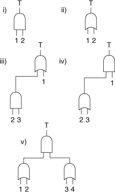
Figure 12-17. Fault tree gates.
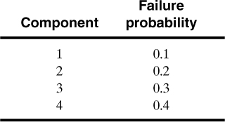
a. Determine an expression for the probability of the top event in terms of the component failure probabilities.
b. Determine the minimal cut sets.
c. Compute a value for the failure probability of the top event. Use both the expression of part a and the fault tree itself.
12-2. The storage tank system shown in Figure 12-18 is used to store process feedstock. Overfilling of storage tanks is a common problem in the process industries. To prevent overfilling, the storage tank is equipped with a high-level alarm and a high-level shutdown system. The high-level shutdown system is connected to a solenoid valve that stops the flow of input stock.
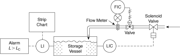
Figure 12-18. Level control system with alarm.
a. Develop an event tree for this system using the “failure of level indicator” as the initiating event. Given that the level indicator fails 4 times/yr, estimate the number of overflows expected per year. Use the following data:
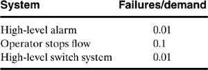
b. Develop a fault tree for the top event of “storage tank overflows.” Use the data in Table 12-1 to estimate the failure probability of the top event and the expected number of occurrences per year. Determine the minimal cut sets. What are the most likely failure modes? Should the design be improved?
12-3. Compute the availability of the level indicator system and flow shutdown system for Problem 12-2. Assume a 1-month maintenance schedule. Compute the MTBC for a high-level episode and a failure in the shutdown system, assuming that a high-level episode occurs once every 6 months.
12-4. The problem of Example 12-5 is somewhat unrealistic in that it is highly likely that the operator will notice the high pressure even if the alarm and shutdown systems are not functioning. Draw a fault tree using an INHIBIT gate to include this situation. Determine the minimal cut sets. If the operator fails to notice the high pressure on 1 out of 4 occasions, what is the new probability of the top event?
12-5. Derive Equation 12-22.
12-6. Show that for a process protected by two independent protection systems the frequency of dangerous coincidences is given by
12-7. A starter is connected to a motor that is connected to a pump. The starter fails once in 50 yr and requires 2 hr to repair. The motor fails once in 20 yr and requires 36 hr to repair. The pump fails once per 10 yr and requires 4 hr to repair. Determine the overall failure frequency, the probability that the system will fail in the coming 2 yr, the reliability, and the unavailability for this system.
12-8. A reactor experiences trouble once every 16 months. The protection device fails once every 25 yr. Inspection takes place once every month. Calculate the unavailability, the frequency of dangerous coincidences, and the MTBC.
12-9. Compute the MTBF, failure rate, reliability, and probability of failure of the top event of the system shown in Figure 12-19. Also show the minimal cut sets.
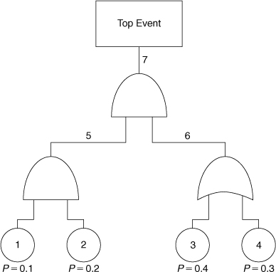
Figure 12-19. Determine the failure characteristics of the top event.
12-10. Determine the MTBF of the top event (explosion) of the system shown in Figure 12-20.
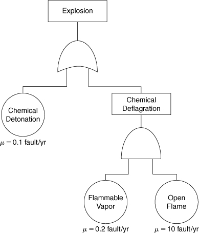
Figure 12-20. Determine the MTBF of the top event.
12-11. Determine P, R, μ, and the MTBF for the top event of the system shown in Figure 12-21. Also list the minimal cut sets.
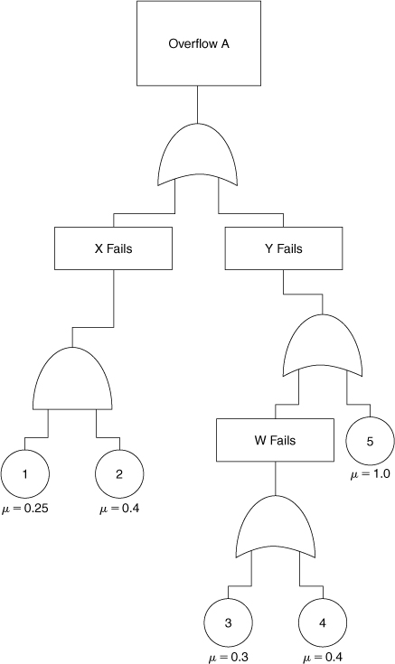
Figure 12-21. Determine the failure characteristics of the top event.
12-12. Determine the failure characteristics and the minimal cut sets for the system shown in Figure 12-22.
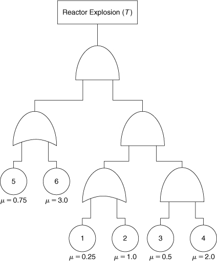
Figure 12-22. Determine the failure characteristics of a reactor explosion.
12-13. Using the system shown in Figure 12-23, draw the fault tree and determine the failure characteristics of the top event (vessel pressure exceeds MAWP).
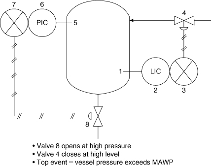
Figure 12-23. A control system to prevent the pressure from exceeding the MAWP.
12-14. Using the system shown in Figure 12-24, draw the fault tree and determine the failure characteristics of the top event (vessel overflows). In this problem you have human intervention; that is, when the alarm sounds, someone turns off valve 7.
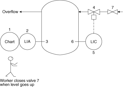
Figure 12-24. Control system to prevent vessel overflow.
12-15. Determine the expected failure rates and MTBFs for control systems with SIL1, SIL2, and SIL3 ratings with PFDs of 10–2, 10–3, and 10–4, respectively.
12-16. Determine the consequence frequency for a regular failure if the system is designed with three IPLs.
12-17. If a regulator has a consequence frequency of 10–1 failure/yr, what will be the frequency if this regulator is given preventive maintenance once per month?
12-18. Determine the consequence frequency of a cooling water system if it is used only 2 months every year and if it is given preventive maintenance each month of operation.
12-19. Assume that a company decides to characterize an acceptable risk as a Category 1 failure every 2 years and a Category 5 failure every 1000 years. Are the following scenarios acceptable or not?
a. Category 4 every 100 years.
b. Category 2 every 50 years.
12-20. Using the results of Problem 12-19,
a. What would you do to move the unacceptable scenarios into the acceptable region?
b. Was the analysis of Problem 12-19 acceptable?
12-21. If a plant has a consequence frequency of 10–2, how many IPLs are needed to reduce this frequency to 10–6?
12-22. What consequence categories do the following scenarios have?
a. Release of 1000 pounds of phosgene.
b. Release of 1000 pounds of isopropanol at 75°F.
c. Potential facility damage of $1,000,000.
12-23. Using the rules for IPLs, list four protective layers that are clearly IPLs.
12-24. If your lockout/tagout procedure has a failure frequency of 10–3 per opportunity, what measures could be taken to reduce this frequency?
12-25. If a specific consequence has two initiating events that give the same consequence, describe the process for determining the frequency of this specific event.
12-26. Determine the MTBF for SIL1–3 systems, if they have PFDs of 10–1, 10–2, and 10–3, respectively. (Note: This is not the same as Problem 12-15.)
12-27. If you have a complex and dangerous plant, describe what you would do to establish which parts of the plant need special attention.
12-28. If you have a plant with poor safety performance, what steps would you take to improve the performance?
12-29. What redundant components should be added to a critical measurement and controller?
12-30. What steps should be taken to decrease the MTBF of a critical control loop?