Appendix C. Detailed Equations for Flammability Diagrams1
Equations Useful for Gas Mixtures
In this appendix we derive several equations that are useful for working with flammability diagrams. Section 6-5 provides introductory material on the flammability diagram. In this section we derive equations proving that:
1. If two gas mixtures R and S are combined, the resulting mixture composition lies on a line connecting the points R and S on the flammability diagram. The location of the final mixture on the straight line depends on the relative moles of the mixtures combined. If mixture S has more moles, the final mixture point will lie closer to point S. This is identical to the lever rule used for phase diagrams.
2. If a mixture R is continuously diluted with mixture S, the mixture composition will follow along the straight line between points R and S on the flammability diagram. As the dilution continues, the mixture composition will move closer and closer to point S. Eventually, at infinite dilution, the mixture composition will be at point S.
3. For systems having composition points that fall on a straight line passing through an apex corresponding to one pure component, the other two components are present in a fixed ratio along the entire line length.
4. The limiting oxygen concentration (LOC) is estimated by reading the oxygen concentration at the intersection of the stoichiometric line and a horizontal line drawn through the LFL. This is equivalent to the equation
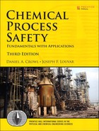
Figure AC-1 shows two gas mixtures, denoted R and S, that are combined to form mixture M. Each gas mixture has a specific composition based on the three gas components A, B, and C. For mixture R the gas composition, in mole fractions, is xAR, xBR, and xCR, and the total number of moles is nR. For mixture S the gas composition is xAS, xBS, and xCS, with total moles nS, and for mixture M the gas composition is xAM, xBM, and xCM, with total moles nM. These compositions are shown in Figure AC-2 with respect to components A and C.
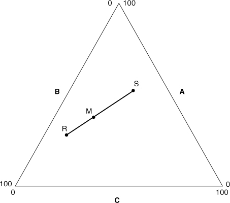
Figure AC-1. Two mixtures R and S are combined to form mixture M.
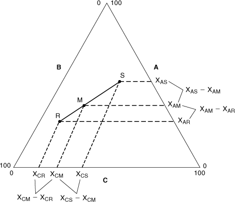
Figure AC-2. Composition information for Figure AC-1.
An overall and a component species balance can be performed to represent the mixing process. Because a reaction does not occur during mixing, moles are conserved and it follows that
A mole balance on species A is given by
A mole balance on species C is given by
Substituting Equation AC-2 into Equation AC-3 and rearranging, we obtain
Similarly, substituting Equation AC-2 into Equation AC-4 results in
Equating Equations AC-5 and AC-6 results in
A similar set of equations can be written between components A and B or between components B and C.
Figure AC-2 shows the quantities represented by the mole balance of Equation AC-7. The mole balance is honored only if point M lies on the straight line between points R and S. This can be shown in Figure AC-2 using similar triangles.2
Figure AC-3 shows another useful result based on Equations AC-5 and AC-6. These equations imply that the location of point M on the straight line between points R and S depends on the relative moles of R and S, as shown.
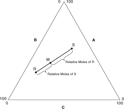
Figure AC-3. The location of the mixture point M depends on the relative masses of mixtures R and S.
These results can, in general, be applied to any two points on the triangle diagram. If a mixture R is continuously diluted with mixture S, the mixture composition follows the straight line between points R and S. As the dilution continues, the mixture composition moves closer and closer to point S. Eventually, at infinite dilution the mixture composition is at point S.
For systems having composition points that fall on a straight line passing through an apex corresponding to one pure component, the other two components are present in a fixed ratio along the entire line length.3 This is shown in Figure AC-4. For this case the ratio of components A and B along the line shown is constant and is given by
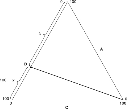
Figure AC-4. The ratio of components A and B is constant along the line shown and is given by x/(100 – x).
A useful application of this result is shown in Figure AC-5. Suppose that we wish to find the oxygen concentration at the point where the LFL intersects the stoichiometric line shown. The oxygen concentration in question is shown as point X in Figure AC-5. The stoichiometric combustion equation is represented by
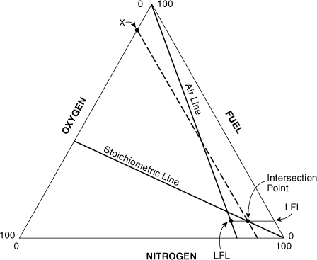
Figure AC-5. Determining the oxygen concentration X at the intersection of the LFL and the stoichiometric line.
where z is the stoichiometric coefficient for oxygen. The ratio of oxygen to fuel along the stoichiometric line is constant and is given by
At the specific fuel concentration of xFuel = LFL it follows from Equation AC-10 that
This result provides a method to estimate the LOC from the LFL. This graphical estimate of the LOC is equivalent to the following:
z is the stoichiometric coefficient for oxygen, given by Equation AC-9, and LFL is the lower flammability limit, in volume percentage of fuel in air.
Equations Useful for Placing Vessels into and out of Service
The equations presented in this section are equivalent to drawing straight lines to show the gas composition transitions. The equations are frequently easier to use and provide a more precise result than manually drawn lines.
The out-of-service fuel concentration (OSFC) is the maximum fuel concentration that just avoids the flammability zone when a vessel is being taken out of service. It is shown as point S in Figure AC-6.
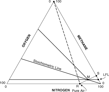
Figure AC-6. Estimating a target fuel concentration at point S for taking a vessel out of service.
For most compounds detailed flammability zone data are not available. In this case an estimate can be made of the location of point S, as shown in Figure AC-6. Point S can be approximated by a line starting at the pure air point and connecting through a point at the intersection of the LFL with the stoichiometric line. Equation AC-7 can be used to determine the gas composition at point S. Referring to Figure AC-2, we know the gas composition at points R and M and wish to calculate the gas composition at point S. Let A represent the fuel and C the oxygen. Then from Figures AC-2 and AC-6 it follows that xAR = 0, xAM = LFL%, xAS is the unknown OSFC, xCM = z(LFL) from Equation AC-11, xCR = 21%, and xCS = 0. Then, by substituting into Equation AC-7 and solving for xAS, we get
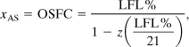
where
OSFC is the out-of-service fuel concentration, that is, the fuel concentration at point S in Figure AC-6,
LFL% is the volume percentage of fuel in air at the lower flammability limit, and z is the stoichiometric oxygen coefficient from the combustion reaction given by Equation AC-9.
Another approach is to estimate the fuel concentration at point S by extending the line from point R through the intersection of the LOC and the stoichiometric line. The result is
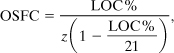
where LOC% is the minimum oxygen concentration in volume percentage of oxygen.
Equations AC-13 and AC-14 are approximations to the fuel concentration at point S. Fortunately, they are usually conservative, predicting a fuel concentration that is less than the experimentally determined OSFC value. For instance, for methane the LFL is 5.0% (Appendix B) and z is 2. Thus Equation AC-13 predicts an OSFC of 9.5% fuel. This is compared to the experimentally determined OSFC of 14.5%. Using the experimental LOC of 12% (Table 6-3), an OSFC value of 14% is determined using Equation AC-14. This is closer to the experimental value but still conservative. For ethylene, 1,3-butadiene, and hydrogen, Equation AC-14 predicts a higher OSFC than the experimentally determined value.
The in-service oxygen concentration (ISOC) is the maximum oxygen concentration that just avoids the flammability zone, shown as point S in Figure AC-7. One approach to estimating the ISOC is to use the intersection of the LFL with the stoichiometric line. A line is drawn from the top apex of the triangle through the intersection to the nitrogen axis, as shown in Figure AC-7. Let A represent the fuel species and C the oxygen. Then, from Figure AC-7 it follows that xAM = LFL%, xAR = 100, xAS = 0, xCM = z(LFL%) from Equation AC-11, xCR = 0, and xCS is the unknown ISOC. Substituting into Equation AC-7 and solving for the ISOC results in
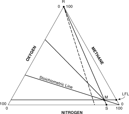
Figure AC-7. Estimating a target nitrogen concentration at point S for placing a vessel into service.
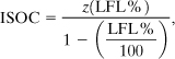
ISOC is the in-service oxygen concentration in volume percentage of oxygen, z is the stoichiometric coefficient for oxygen given by Equation AC-9, and
LFL% is the fuel concentration at the lower flammability limit, in volume percentage of fuel in air.
The nitrogen concentration at point S is equal to 100 – ISOC.
An expression to estimate the ISOC using the intersection of the minimum oxygen concentration and the stoichiometric line can also be developed using a similar procedure. The result is
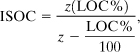
where LOC% is the limiting oxygen concentration in volume percentage of oxygen.
Although these calculations are useful for making good estimates, direct, reliable experimental data under conditions as close as possible to process conditions are always recommended.