
Agent-Based Macroeconomics✶
Herbert Dawid⁎,1; Domenico Delli Gatti†,‡ ⁎Department of Business Administration and Economics and Center for Mathematical Economics, Bielefeld University, Bielefeld, Germany
†Complexity Lab in Economics (CLE), Department of Economics and Finance, Università Cattolica del Sacro Cuore, Italy
‡CESifo Group Munich, Germany
1Corresponding author. email address: [email protected]
Abstract
This chapter surveys work dedicated to macroeconomic analysis using an agent-based modeling approach. After a short review of the origins and general characteristics of this approach a systemic comparison of the structure and modeling assumptions of a set of important (families of) agent-based macroeconomic models is provided. The comparison highlights substantial similarities between the different models, thereby identifying what could be considered an emerging common core of macroeconomic agent-based modeling. In the second part of the chapter agent-based macroeconomic research in different domains of economic policy is reviewed.
Keywords
Agent-based macroeconomics; Aggregation; Heterogeneity; Behavioral rules; Business fluctuations; Economic policy
1 Introduction
Starting from the early years of the availability of digital computers, the analysis of macroeconomic phenomena through the simulation of appropriate micro-founded models of the economy has been seen as a promising approach for Economic research. In an article in the American Economic Review in 1959 Herbert Simon argued that
“The very complexity that has made a theory of the decision-making process essential has made its construction exceedingly difficult. Most approaches have been piecemeal-now focused on the criteria of choice, now on conflict of interest, now on the formation of expectations. It seemed almost utopian to suppose that we could put together a model of adaptive man that would compare in completeness with the simple model of classical economic man. The sketchiness and incompleteness of the newer proposals has been urged as a compelling reason for clinging to the older theories, however inadequate they are admitted to be. The modern digital computer has changed the situation radically. It provides us with a tool of research—for formulating and testing theories—whose power is commensurate with the complexity of the phenomena we seek to understand. [...] As economics finds it more and more necessary to understand and explain disequilibrium as well as equilibrium, it will find an increasing use for this new tool and for communication with its sister sciences of psychology and sociology.” (Simon, 1959, p. 280).
This quote, which calls for an encompassing macroeconomic modeling approach building on the interaction of (heterogeneous) agents whose expectation formation and decision making processes are based on empirical and psychological insights, might be seen as the first formulation of a research agenda, which is now referred to as “Agent-Based Macroeconomics.” Cohen (1960) provides a very insightful discussion of the potential and the challenges of the use of computer simulations for the development of a behavioral theory of the firm, as well as for the analysis of aggregate economic models. An early example of an actual simulation-based macroeconomic model is the evolutionary model of economic growth discussed in Nelson and Winter (1974) and Nelson et al. (1976). In the 1970s micro-founded simulation models of the Swedish economy (the MOSES model, see Eliason, 1977, 1984) and the US economy (the “Transactions Model”, see Bergman, 1974; Bennett and Bergmann, 1986) have been developed as a tool for the analysis of certain economic policy measures. Although calibrated for specific countries, the structure of these models was rather general and as such they can be seen as very early agent-based macroeconomic models.
At the same time, starting in the 1970s the attention of the mainstream of macroeconomic research has shifted towards (dynamic) equilibrium models as a framework for macroeconomic studies and policy analyses. At least in their original form these models are built on assumptions of representative agents, rational expectations, and equilibrium based on inter-temporally optimal behavior of all agents. The clear conceptual basis, as well as the relatively parsimonious structure of these models, and the fact that they address the Lucas critique has strongly contributed to their appeal and has resulted in a large body of work dedicated to this approach. In particular, these models have become the workhorse for macroeconomic policy analysis.
Nevertheless, already early in this development different authors have pointed out numerous problematic aspects associated with using such models, in particular Dynamic Stochastic General Equilibrium (DSGE) models, for economic analysis and policy studies. Kirman (1992) nicely summarizes results, showing that in general aggregate behavior of a heterogeneous set of (optimizing) agents cannot be interpreted as the optimal decision of a representative agent and that, even in cases where it can, the sign of effects of policy changes on the utility of that representative agent might be different from the sign of the induced utility changes of all agents in the underlying population, which makes the interpretation of welfare analysis in representative agent models problematic. Furthermore, an extensive stream of literature has shown that under reasonable informational assumptions no adjustment processes ensuring general convergence to equilibrium can be constructed (see Kirman, 2016). Hence, the assumption of coordination of all agents in an equilibrium is very strong, even if a unique equilibrium exists, which in many classes of models is not guaranteed. As argued, e.g., in Howitt (2012) this assumption also avoids addressing coordination issues in the economy, which are essential for understanding the phenomena like the emergence of crises and also the impact of policies. Similarly, the assumption that all agents have rational expectations about the future dynamics of the economy has been criticized as being rather unrealistic, and indeed there is little experimental or empirical evidence suggesting that the evolution of expectations of agents is consistent with the rational expectations assumption (see, e.g., Carroll, 2003 or Hommes et al., 2005).
From a more technical perspective, studies in the DSGE literature typically rely on local approximations of the model dynamics around a steady state (e.g., log-linearization) and thereby do not capture the full global dynamics of the underlying model. This makes it problematic to properly capture global phenomena like regime changes or large fluctuations in such a framework. Business cycles and fluctuations are driven by shocks to fundamentals or expectations, whose structure is calibrated in a way to match empirical targets. Hence, the mechanisms actually generating these fluctuations are outside the scope of the model and therefore the model can only be used to study propagation of shocks, but is silent about which mechanisms generate such phenomena and which measures might reduce the risk of the emergence of cycles and downturns in the first place.
In the aftermath of the crises developing after 2007, policy makers, as well as economists, have acknowledged that several of the properties mentioned above substantially reduce the ability of standard DSGE models to inform policy makers about suitable responses to the unfolding economic downturn. New generations of DSGE-type models have been developed addressing several of these issues, in particular introducing more heterogeneity (see Ragot, 2018 in this handbook), heterogeneous non-rational expectations (see Branch and McGough, 2018 in this handbook) or the feedback between real and financial dynamics (e.g., Benes et al., 2014); however, also in each of these extensions several of the points discussed above, which seem intrinsic associated with this approach, still apply.1
Related to these new developments also a stream of literature has emerged, which, although relying on the backbone of a standard DSGE-type model, in certain parts of the model incorporates explicit micro-level representations of the (local) interaction of agents and relies on (agent-based) simulation of the emerging dynamics. Although these contributions (e.g., Anufriev et al., 2013; Arifovic et al., 2013; Assenza and Delli Gatti, 2013, 2017; Lengnick and Wohltmann, 2016) can be considered to be part of the agent-based macroeconomic literature, they are more hybrid in nature and this literature is treated in the chapter by Branch and McGough (2018) in this handbook, rather than in this chapter.2
The agent-based approach to macroeconomic modeling, which has started to attract increasing attention from the early 2000s onwards, is similar in spirit to Simon's quote above and hence differs in several ways from mainstream dynamic equilibrium models. In agent-based macroeconomic models, different types of heterogeneous agents endowed with behavioral and expectational rules interact through explicitly represented market protocols and meso- as well as macroeconomic variables are determined by actual aggregation of the output in this population of agents. They are mainly driven by the desire to provide empirically appealing representations of individual behavior and interaction patterns at the micro level and at the same time to validate the models by comparing the characteristics of their aggregate level output with empirical data. The global dynamics of the models are studied relying on (batches of) simulation runs and typically no ex-ante assumptions about the coordination of individual behavior are made.
Already early contributions to this stream of literature have shown that such models can endogenously generate fluctuations resembling actual business cycles without relying on external shocks (e.g., Dosi et al., 2006) and have highlighted, before the outbreak of the crises of 2007, mechanisms by which contagion (e.g., through credit networks) and feedback between the real and financial side of the economy can induce instability and sudden downturns (see Battiston et al., 2007). These properties, together with the ability to incorporate a wide range of behavioral assumptions and to represent institutional characteristics, which might be relevant for the analysis of actual policy proposals, have fostered interest of policy makers for agent-based macroeconomic modeling3 and resulted in a vast increase in research in this area in general, and in agent-based policy analysis in particular. As has to be expected from a new emerging paradigm, the evolution of the field has progressed in several weakly coordinated streams, and in light of the large body of work that has been produced so far, a systematic review of the progress that has been made seems to be in order. This chapter is an attempt to provide such a review.
1.1 Complexity and Macroeconomics
The notion of complexity is general enough to encompass a broad class of phenomena and models in nature and society. We interpret complexity as an attribute of a system. In particular, following the approach pioneered at the Santa Fe Institute by an interdisciplinary group of prominent scientists, complex adaptive systems (CAS) are systems consisting of a large number of “coupled elements the properties of which are modifiable as a result of environmental interactions. [...] In general complex adaptive systems are highly non-linear and are organized on many spatial and temporal scales” (cited from Cowan and Feldmann in Fontana, 2010, p. 173).
Macroeconomic dynamics are characterized by the interaction of a large number of heterogeneous individuals who take a plethora of decisions of different kinds to produce and exchange a large variety of goods, as well as information. These transactions are governed by institutional rules which might vary significantly between different regions, industries, time periods, and other contexts. Based on this, economic systems must certainly be seen as very complex adaptive systems. This makes it extremely challenging to develop appropriate models for studying economic systems and to derive any insights of general validity about the (future) dynamics of key economic variables or the effect of certain economic policy measures.
In order to study CAS, a natural tool is an Agent Based Model (ABM), i.e., a model in which a multitude of (heterogeneous) elements or objects interact with each other and the environment. The single most important feature of an ABM is the autonomy of the elements, i.e., the absence of a centralized (“top down”) coordinating or controlling mechanism. ABMs are, by construction, computationally intensive. The output of the model typically cannot be determined analytically but must be computed and consists of simulated time series. A key feature of CAS is that it often gives rise to emerging properties, i.e., stable, orderly aggregate structures resulting from the interaction of the agents' behavior. A phenomenon is emergent whenever the whole achieves properties which its elements, if taken in isolation, do not have.
1.2 The Agent-Based Approach to Macroeconomic Modeling
Agent-based Computational Economics (ACE) is the application of AB modeling to economics or: “The computational study of economic processes modeled as dynamic systems of interacting agents.” (Tesfatsion, 2006). Surveys of the ample literature on ACE work in different areas of Economics are provided in the second volume of the Handbook of Computational Economics (Tesfatsion and Judd, 2006). It is worthwhile noting that in this handbook no separate chapter on agent-based macroeconomics was included, which is a signal of the limited work in this area that has been completed before 2006.
A defining feature of macroeconomic ABMs (MABMs) is that although concerned with the dynamics of aggregate economic variables, such as GDP, consumption, etc., they explicitly capture the micro-level interaction of different types of heterogeneous economic agents and allow computing the aggregate variables “from the bottom up”, i.e., summing individual quantities across agents. The bottom-up approach to macroeconomics consists therefore in deducing the macroscopic patterns and phenomena in terms of a multitude of elementary microscopic objects (microeconomic variables) interacting according to certain rules and protocols.
Developing and using an MABM typically requires a number of steps:
- • Model Design and Theory:
- ∘ determine the type of agents included to be in the model (households, firms, banks, etc.);
- ∘ for each agent of each type define the set of decisions to be taken, the set of internal states (e.g., wealth, skills, savings, etc.), structure of each decision rule (inputs, how is decision made), the potential information exchange with other agents and the potential dynamic adjustment of internal states and decision rules; decide on the theoretical, empirical or experimental foundations on which these choices are based;
- ∘ define interaction protocols for all potential interactions.
- • Codification: translate the rules into computer code, do proper testing of the code (e.g., unit testing) to ensure proper implementation of the model.
- • Parameter Choice and Validation: estimate and calibrate the parameters; run simulations; analyze the emerging properties of the simulated data, both at the cross-sectional level (e.g., firms' size distribution) and at the macroeconomic level (GDP growth and fluctuations, inflation/unemployment trade-off); compare these properties with real world “stylized facts.”
- • Model Analysis: study the effects of changes in key model parameters (e.g., policy parameters) based on proper statistical analysis of the output of batch runs across different parameter settings; use micro-level simulation data to highlight the mechanisms responsible for the observed findings and to foster economic intuition for the findings.
Several properties are common to MABMs and have been encountered in many agent-based models in Economics, among them several of the models reviewed in this chapter. First and foremost, in MABMs GDP tends to self-organize towards a growth path with endogenously generated fluctuations, such that business cycles are driven by the mechanics of the model rather than by properties of exogenous shocks. Furthermore, these models typically generate persistent heterogeneity of agents, giving rise to stable population distributions of firm size, productivity, profitability, growth rate or household income and thereby can reproduce also empirical patterns with respect to distributions of such variables. In particular, distributions with fat tails, which are observed for many real world variables (see, e.g., Axtell, 2018 in this handbook), have been reproduced in many instances by MABMs. Being able to jointly reproduce empirical stylized facts with respect to time series properties and distributional properties at different levels of aggregation is certainly a very appealing feature of MABMs, which is hard to obtain in the framework of alternative macroeconomic modeling approaches.
Many MABMs are characterized by externalities and nonlinearities (due to interaction), which generate dynamic processes with positive feedbacks. Due to the presence of such feedbacks path dependencies might arise such that initial conditions or random events in the transient phase can have decisive impact on the long run dynamics. These properties of MABMs are also the basis for endogenously generating extreme events, like crashes and economic crises, as well as fast transitions between different quasi-stable regimes. MABMs capture the actual dynamic mechanisms generating such potential fast economic transitions and therefore are natural tools to study how to prevent or mollify economic crises, e.g., through appropriate institutional designs or policy measures. Generally speaking, the fact that agent-based models allow for global analysis of macroeconomic dynamics in frameworks which endogenously generate dynamic and cross-sectoral patterns, which closely resemble empirical data, arguably is a main reason for the appeal of this approach.
1.3 Behavior, Expectations, and Interaction Protocols
In dynamic equilibrium models, individual behavior is typically determined by the optimal solution of some (dynamic) optimization problem an agent with rational expectations faces. Quite differently, in agent-based macroeconomic models it is not assumed that the economy is in equilibrium and that individuals have rational expectations. Hence, the agents in the model, similarly to real-world decision makers, are “necessarily limited to locally constructive actions, that is, to actions constrained by their interaction networks, information, beliefs, and physical states.” (Sinitskaya and Tesfatsion, 2015, p. 152). The design of behavioral rules determining such locally constructive actions is a crucial aspect of developing an agent-based macroeconomic model. The lack of an accepted precise common conceptual or axiomatic basis for the modeling of bounded rational behavior has raised concerns about the “wilderness of bounded rationality” (Sims, 1980); however, agent-based modelers have become increasingly aware of this issue, providing different foundations for their approaches to model individual behavior.
Generally speaking, in many MABMs the design of the behavioral rules builds on the extensive psychological and empirical literature showing the prevalence of relatively simple heuristics and rules of thumb for making decisions, including economic decisions in complex environments (see, e.g., Gigerenzer and Gaissmaier, 2011; Artinger and Gigerenzer, 2016). Such rules might be derived from optimization within the framework of a simplified internal model of the surrounding environment, or might evolve over time based on adjustment dynamics that take into account which types of rules generate desirable results for the decision maker.4 In a number of agent-based models the chosen behavioral rules are strongly motivated by experimental5 or empirical observations of how actual decision makers behave in certain types of decision problems.6 As will become clear in our survey below, the literature shows substantial heterogeneity with respect to the approach that underlies the design of the behavioral rules. Similar statements apply to the expectation formation of agents. The absence of the assumption of rational expectations typically gives rise to models with evolving heterogeneous expectations and also in this domain different approaches have been followed.
Given the heterogeneity in the way decision making and expectation formation are modeled, it would be desirable to have a clear understanding of how robust results obtained in the framework of a certain model are with respect to the use of alternative plausible behavioral rules. A step in this direction is taken by Sinitskaya and Tesfatsion (2015), who compare in a simple macroeconomic framework how key outcomes of the model compare across settings with different types of decision rules; however, in particular in large macroeconomic models such robustness tests are not feasible and the chosen design of the behavioral rules might therefore be an important determinant of the model output.
In most macroeconomic agent-based models the interaction of the different agents in markets or other interaction structures are governed by explicit protocols that represent the institutional design of the considered economic system. This allows capturing details of the institutional setting and also allows representing in a natural way potential rationing of both market sides, as well as the occurrence of frictions in a market. The degree of detail with which the interactions structures in different markets are described, of course, varies substantially across the agent-based macroeconomic models that have been developed and is strongly influenced by the main focus of the model.
1.4 Outline of the Chapter
In this chapter we discuss the main developments in Agent-Based Macroeconomics during the last decade. The treatment is essentially split into two parts. In the first part, consisting of Sections 2 and 3, we focus on the design of macroeconomic agent-based models. In particular, in Section 2 we address in some detail several main challenges of macroeconomic agent-based modeling, in particular the design of the behavioral rules of different types of agents for several of the most crucial decisions to be taken. We illustrate how these challenges were treated in eight macroeconomic agent-based models that have been well perceived in the literature. In Section 3, we provide more of a bird's-eye view on these model by summarizing the detailed discussion of Section 2 and providing a systematic comparison of these eight MABMs along a larger number of modeling dimensions. Section 3 also contains a discussion of the way these models have been linked to empirical data. The discussion in Section 3 is based on Tables A1 and A2, provided in Appendix A, in which a short summary of the main features of all eight models is given. Overall, we hope that Sections 2 and 3 of the chapter do not only provide a survey of the literature, but are also helpful in identifying what could be considered a common core of macroeconomic agent-based modeling. The second part of the chapter, essentially Section 4, provides an overview of macroeconomic policy analyses that have been carried out using agent-based models. Although the eight models discussed in Sections 2 and 3 are the basis for a considerable fraction of this policy oriented work, numerous studies reviewed in Section 4 do not fall into this category. This highlights the breadth of work in agent-based macroeconomics during the last years and the fact that a chapter like this, due to space constraints, cannot properly capture the full status of the literature. The chapter concludes with some remarks about challenges for the future development of this line of research and about areas in which, in our opinion, the potential for agent-based analysis is particularly high.
2 Design of Agent-Based Macroeconomic Models
2.1 Families of MABMs
Macroeconomic Agent-Based Models (MABMs) can be classified according to different criteria. First of all, we can distinguish between large, medium sized, and small MABMs.
Medium sized and large MABMs feature at least three agent types – households, firms, and banks – interacting at least on five markets: consumption goods (C-goods hereafter), capital or investment goods (K-goods), labor, credit, deposits. Small MABMs generally feature just two types of agents – households and firms – interacting on two markets: C-goods and labor.
Some MABMs are able to replicate growth, i.e., a long-run exponential trend around which actual GDP irregularly fluctuates, some other focus only on the short run, i.e., they can replicate only business fluctuations.
In this section and the next, we will focus on medium-sized MABMs, grouping them into seven families:
- 1. The framework developed by Ashraf, Gershman, and Howitt (AGH hereafter)7;
- 2. The family of models proposed by Delli Gatti, Gallegati, and coauthors in Ancona and Milan exploiting the notion of Complex Adaptive Trivial Systems (CATS)8;
- 3. The framework developed by Dawid and coauthors in Bielefeld as an offspring of the EURACE project,9 known as Eurace@Unibi (EUBI)10;
- 4. The EURACE framework maintained by Cincotti and coauthors in Genoa (EUGE)11;
- 5. The Java Agent based MacroEconomic Laboratory developed by Salle and Seppecher (JAMEL)12;
- 6. The family of models developed by Dosi, Fagiolo, Roventini, and coauthors in Pisa, known as the “Keynes meeting Schumpeter” framework (KS)13;
- 7. The LAGOM model developed by Jaeger and coauthors.14
We will also present the relatively simple small model developed by Lengnick (LEN) for comparison.15 Key references for these models are given in Tables A1 and A2.
By selecting these eight families of models, on the one hand, we tried to pick those that seem to have had the strongest impact on the literature and have been used as the basis for interesting economic analyses and policy experiments, and, on the other hand, also present some variety to show the range of approaches that have been developed to deal with the challenges of agent-based macroeconomic modeling. Clearly, any such selection is highly subjective and, as will also become clear in the discussion of agent-based policy analyses in Section 4, the selection made here misses a substantial number of important contributions to this area. Nevertheless, we believe that presenting such a survey is not only useful for newcomers to the field, but also helps to provide transparency about the status of the field of agent-based macroeconomics. Due to the rather complex structure of many models in this field, which often makes a full model description rather lengthy, such transparency is not easy to obtain.
The interested reader who ventures for the first time into this literature may feel the excitement of exploring a new world and, at the same time, the disorientation and discouragement of getting lost in the wilderness. At first sight, in fact, these models look very different from one another so that it's extremely difficult for the beginner to “see the forest” above and beyond a wide variety of trees. In our opinion, however, there are common denominators, both in the basic architecture of the models and in the underlying theory of the way in which agents form behavioral rules and interact on markets.
2.2 A Map of this Section
Let us set the stage by considering the architecture of an MABM. The economy is populated, at a minimum, by households and firms (as in LEN). Medium-sized MABMs are populated also by banks.
Households supply labor and demand C-goods. In most MABMs, households are “surplus units”, i.e., net savers. Savings are used to accumulate financial wealth.
The corporate sector consists, at a minimum, of producers of C-goods (C-firms). Most MABMs, however, are now incorporating also producers of K-goods (K-firms). C-firms demand labor and K-goods in order to produce and sell C-goods to households. K-firms supply K-goods to C-firms.
In most MABMs firms are “deficit units”, i.e., firms' internal funds may not be sufficient to finance costs. Therefore they resort to external finance to fill the financing gap. In most MABMs, external finance coincides with bank loans. Banks receive deposits from households and extend loans to firms.
In small MABMs, such as LEN, there are markets for C-goods and labor. In medium-sized MABMs, there are typically markets for C-goods, K-goods, labor, credit, and deposits.16 Given this architecture, we can allocate agents in markets according to the grid shown in Table 1. Each column of the table represents a group of agents, each row a market. For instance, H/C/d represents Households acting on the market for C-goods on the side of demand.
Table 1
H stands for households; F denotes firms; B stands for banks; N denotes the labor market; L denotes the market for loans; and A denotes the market for assets
| Households | Firms | Banks | |
|---|---|---|---|
| C-goods | H/C/d | F/C/s | |
| K-goods | F/K/d,s | ||
| Labor | H/N/s | F/N/d | |
| Credit | F/L/d | B/L/s | |
| Assets | H/A/d | F/A/s |

Instead of reviewing the models one after another, in each of the following subsections we will discuss the characterizations that the proponents of different MABMs adopt to describe the behavioral rules that each type of agent (on the columns) follows in each of the different markets the agent is active (on the rows). We will also devote some space to the description of the interaction of buyers and sellers on markets (market protocols) which Tesfatsion labels “procurement process.”17
We aim at bringing to the fore the similarities among different MABMs. As mentioned above, assumptions and modeling choices come from a variety of sources, first and foremost from the empirical and experimental evidence. It is worth noting, moreover, that these assumptions have a varying degree of kinship with the current macroeconomic literature. MABMs are not developed in a vacuum, the shapes of their building blocks come also from the theoretical debate in macroeconomics. For this reason, at the beginning of each subsection, we will succinctly present the microeconomic backbone of a standard New Keynesian DSGE (NK-DSGE) model (the standard model hereafter) pertaining to that class of agents,18 then present the behavioral rules and market protocols of MABMs concerning the same class. In this way we can discuss similarities and differences (i) between the standard model and the MABMs, and (ii) among MABMs. In order to make the comparison easier, we will adopt our own notation, which will be uniform across different MABMs. We will also slightly simplify the analytical apparatus of a specific MABM under review to make the modeling choices starker in the eyes of the reader. Notice finally that we will consider each MABM as the result of a collective effort (with the exception of LEN). Hence we will conjugate a verb describing the action of the group behind the label of each MABM in the third person plural. To foster readability, we provide in Appendix B a list of symbols with their meaning that are used in this section.
In our presentation of MABMs, due to space limitations, we will not discuss three relevant features.
The first concerns the sequence of events, which may differ from one model to another. By construction, MABMs are recursive sequential models. Agents decide on the desired level of their choice variables (planned level) following behavioral rules and then enter markets one after another in order to implement those decisions by suitable transactions. Search of trading opportunities and matching of supply and demand occur in fully decentralized markets, i.e., in the absence of a top-down mechanism to enforce equilibrium. Therefore, transactions typically occur at prices which do not clear the market. This may cause a disruption of plans, which must be revised accordingly.
Consider, for instance, a C-firm. Once the quantity to be produced has been established, the firm determines desired employment. If desired employment is greater than the current workforce, the firm tries to hire new workers by posting vacancies. It may not be able to fill the vacancies, however, because not enough workers will visit the firm or accept the position.19 In this case, the firm has to downsize its production plans. Generally, due to unexploited trading opportunities, three constraints may limit the implementation of decisions, e.g., firms may be unable to (i) find enough external funds to fill the financing gap and/or (ii) hire enough workers and/or (iii) acquire enough capital to implement the desired level of production.
The second feature concerns time discretization. By construction, in MABMs time is discrete. MABMs can differ, however, as far as the minimal time unit is considered (a day, a week, a month, a quarter). Moreover, transactions can occur at different time scales. For instance, in LEN C-goods are traded every day but labor services are traded on a monthly basis. In the following, for simplicity we will not be specific on the time unit which will be referred to with the generic term “a period.”
The third feature concerns the characterization of interaction. A few MABMs are networked, i.e., they have an explicit network structure: agents are linked by means of trading relationships which take the form of persistent partnerships. In LEN, for instance, each household trades with a finite set of firms.20 Most of the MABMs we will consider below, however, do not assume a fixed network of trading relationships. Partners in a trade today may not trade again tomorrow. In a sense, trading relationships de facto connect people in a network which is systematically reshuffled every period.21
2.3 Households
In the following, we will consider a population of H households. Variables pertaining to the hth household will be denoted with the suffix h. Households may be active or inactive on the labor market. If active, they supply labor (in most MABMs, labor supply is exogenous). In some MABMs, households searching the labor market have a reservation wage, which may be constant or decreasing with the length of the unemployment spell. If employed, the household earns a wage. In some MABMs, if unemployed, the household receives an unemployment subsidy, which amounts to a fraction of the wage of employed households.
Households are also firm owners. Firm ownership may be limited to a fraction of inactive households or spread somehow also to active households. As a firm owner, the household receives dividends. Current income is the sum of the wage bill and dividends. Households purchase C-goods. Generally, households are surplus units, i.e., they do not get into debt. Unspent income is saved and generates financial wealth. In most MABMs, financial wealth consists of bank deposits only.
In LEN, households are linked in a network of trading relationships to a finite set of firms from which they buy C-goods and firms for which they work. Since there are no banks, households hold wealth in liquid form (money holding).
In AGH, each household (“person”) is denoted by the type (i,j)![]() where i is the household's labor/product type and j are the types of goods the household wants to consume. By assumption the household consumes only two goods, different from the good it can produce. The product type is isomorphic to the labor type.22 A household of type i can be a worker if employed by a firm (“shop”) of the same type. If a worker, she earns a wage. Otherwise, the household can be a firm owner.
where i is the household's labor/product type and j are the types of goods the household wants to consume. By assumption the household consumes only two goods, different from the good it can produce. The product type is isomorphic to the labor type.22 A household of type i can be a worker if employed by a firm (“shop”) of the same type. If a worker, she earns a wage. Otherwise, the household can be a firm owner.
In the CATS framework, households can be either workers or “capitalists.” Workers supply labor, earn a wage (if employed), consume, and save. Capitalists are the owners of firms. For simplicity there is one capitalist per firm. Capitalists earn dividends (if the firm is profitable), consume, and save (therefore they behave as rentiers). Both workers and capitalists accumulate their savings in the form of deposits at banks. If the firm goes bankrupt, the owner of the bankrupt firm employs his personal wealth to provide equity to the entrant firm. In other words, the capitalist is de facto recapitalizing the defaulting firm to make it survive.
In KS, EUBI, EUGE, and LAGOM, each household supplies labor and owns firms at the same time. This alternative approach poses the problem of attributing ownership rights, dividends, and recapitalization commitments to heterogeneous households. For instance, in EUBI, the household holds financial wealth in the form of deposits at banks and an index of stocks which define property rights and the distribution of dividends.
In JAMEL, some of the households (chosen at random) are firm owners and remain firm owners for a certain time period (typically a run of a simulation).
2.3.1 The Demand for Consumption Goods
In this section we will first recall the basic tenets of the standard model of household's consumption/saving decisions, which we will refer to as the Life Cycle/Permanent Income (LCPI) benchmark. We will then present the most general specification of the consumption behavioral rule which we can extract from the MABM literature. The specific behavioral rules adopted by different MABMs can be conceived as special cases of this general specification.
The Life Cycle/Permanent Income Benchmark
The standard approach to households' behavior (incorporated in NK-DSGE models) is based on “two-stage budgeting.” In the first stage, the representative infinitely lived household maximizes expected lifetime utility subject to the intertemporal budget constraint, determining the optimal size of consumption expenditure Ch,t![]() , which we will sometimes refer to hereafter as the consumption budget.
, which we will sometimes refer to hereafter as the consumption budget.
In the second stage the household determines the composition of Ch,t![]() , i.e., the fraction Ci,h,t/Ch,t
, i.e., the fraction Ci,h,t/Ch,t![]() for each variety i=1,2,…,Fc
for each variety i=1,2,…,Fc![]() where Fc
where Fc![]() is the cardinality of the set of C-goods (and of C-firms).23
is the cardinality of the set of C-goods (and of C-firms).23
As far as the first stage is concerned, optimal consumption turns out to be a function of expected future consumption EtCh,t+1![]() and the real interest rate r (consumption Euler equation).
and the real interest rate r (consumption Euler equation).
Notice now that consumption expenditure is equal by definition to permanent income, Ch,t=Yph,t![]() . Hence, after some algebra, we get
. Hence, after some algebra, we get
(1) Ch,t=ˆr(Whh,t+Wfh,t)
where ˆr=ˆR−1![]() is the (net, real) interest rate, Whh,t
is the (net, real) interest rate, Whh,t![]() is human capital, and Wfh,t
is human capital, and Wfh,t![]() is financial wealth. Eq. (1) can be interpreted as a benchmark Life Cycle/Permanent Income (LCPI) consumption function. In this framework, by construction, the consumption budget is equal to the annuity value of total (financial and human) wealth.
is financial wealth. Eq. (1) can be interpreted as a benchmark Life Cycle/Permanent Income (LCPI) consumption function. In this framework, by construction, the consumption budget is equal to the annuity value of total (financial and human) wealth.
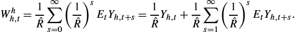
Human capital, in turn, is defined as the discounted sum of current income and expected future incomes accruing to the household:
(2) Whh,t=1ˆR∞∑s=0(1ˆR)sEtYh,t+s=1ˆRYh,t+1ˆR∞∑s=1(1ˆR)sEtYh,t+s.
Substituting (2) into (1), the LCPI consumption function becomes
(3) Ch,t=ˆrˆRYh,t+ˆrˆR∞∑s=1(1ˆR)sEtYh,t+s+rWfh,t.
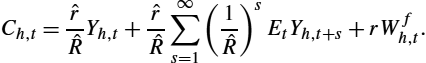
In words, consumption is a linear function of current and expected future incomes and of financial wealth.
By definition, in the LCPI benchmark, Wfh,t+1=ˆRWfh,t+Yh,t−Ch,t![]() . Therefore savings, i.e., the change in financial wealth Sh,t=Wfh,t+1−Wfh,t
. Therefore savings, i.e., the change in financial wealth Sh,t=Wfh,t+1−Wfh,t![]() , turns out to be equal to Sh,t=ˆrWfh,t+Yh,t−Ch,t
, turns out to be equal to Sh,t=ˆrWfh,t+Yh,t−Ch,t![]() . Since consumption is equal to permanent income, savings can be specified as follows:
. Since consumption is equal to permanent income, savings can be specified as follows:
(4) Sh,t=ˆrWfh,t+(Yh,t−Yph,t)
where the expression in parentheses is transitory income. All the income in excess of permanent income will be saved and added to financial wealth. If, on the other hand, current income falls short of permanent income, the household will stabilize consumption by decumulating financial wealth.
As far as the second stage is concerned, it is easy to show that in a Dixit–Stiglitz framework the (optimal) fraction of each good in the bundle is
(5) Ci,h,tCh,t=(Pi,tPt)−ε
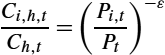
where Pi,t![]() is the price of the ith variety, Pt
is the price of the ith variety, Pt![]() is the general price level,24 and ε is the absolute value of the price elasticity of demand. In words, the fraction of the consumption budget allocated to each variety is a decreasing function of the relative price Pi,tPt
is the general price level,24 and ε is the absolute value of the price elasticity of demand. In words, the fraction of the consumption budget allocated to each variety is a decreasing function of the relative price Pi,tPt![]() .
.
Generally, households are assumed to be identical. If household members are heterogeneous (for instance, because of the employment status, or the level and the source of income), in standard models complete markets are assumed so that idiosyncratic risk can always be insured. Within the household, “full consumption insurance” follows from the assumption that household members pool together their incomes (wages, unemployment subsidies, dividends) and consume the same amount in the same proportions. Thanks to this assumption, heterogeneity, albeit present, is irrelevant because the household may still be dealt with as a unique (representative) agent. If idiosyncratic income risk is uninsurable, then heterogeneity cannot be assumed away.25
The Agent Based Approach to Consumption/Saving Decisions
A two stage procedure is also generally adopted in MABMs. In the first stage household h determines the consumption budget Ch,t![]() , i.e., the amount of resources (income, wealth) to be allocated to consumption expenditure. In the second stage the household determines the composition of the bundle of consumption goods, i.e., the quantities Ci,h,t
, i.e., the amount of resources (income, wealth) to be allocated to consumption expenditure. In the second stage the household determines the composition of the bundle of consumption goods, i.e., the quantities Ci,h,t![]() , i=1,2,…,Fc
, i=1,2,…,Fc![]() of the goods which enter the consumption bundle. Notice, however, that in general agents do not follow explicit optimization procedures. Markets are generally incomplete and within-household consumption insurance is ruled out.
of the goods which enter the consumption bundle. Notice, however, that in general agents do not follow explicit optimization procedures. Markets are generally incomplete and within-household consumption insurance is ruled out.
The Choice of the Consumption Budget
As far as the first stage is concerned, the most general behavioral rule adopted to set the consumption budget in the MABM literature can be specified as follows:
(6) Ch,t=chWhh,t+cfWfh,t
where Wfh,t![]() is the household's financial wealth (deposited at the bank and/or invested in financial assets), Whh,t
is the household's financial wealth (deposited at the bank and/or invested in financial assets), Whh,t![]() is human capital, ch
is human capital, ch![]() and cf
and cf![]() are propensities to consume, both positive and smaller than one. In words, consumption is a linear function of human and financial wealth.
are propensities to consume, both positive and smaller than one. In words, consumption is a linear function of human and financial wealth.
By definition, Wfh,t=ˆRWfh,t−1+Yh,t−Ch,t![]() and Sh,t=Wfh,t−Wfh,t−1
and Sh,t=Wfh,t−Wfh,t−1![]() . Consumption is defined as in (6). Hence, in a generic MABM savings turn out to be
. Consumption is defined as in (6). Hence, in a generic MABM savings turn out to be
(7) Sh,t=Yh,t+(ˆr−cf)Wfh,t−1−chWhh,t.
If positive, savings increase financial wealth. In some MABMs saving can be involuntary: it may happen that the household cannot find enough consumption goods at the limited number of firms it visits. Savings will turn negative, i.e., the household will decumulate financial wealth, if the consumer does not receive income, for instance, because a worker becomes unemployed and/or financial income (interest payments on financial wealth) is too low. In most MABMs, household do not get into debt so that consumption smoothing is limited or absent (in the jargon of NK-DSGE models, asset market participation is limited).
Specifications of the general rule (6) differ from one MABM to another.
AGH set ch=cf=c![]() . Moreover, they define human capital as the capitalized value of permanent income Whh,t=khYph,t
. Moreover, they define human capital as the capitalized value of permanent income Whh,t=khYph,t![]() where kh
where kh![]() is a capitalization factor.26 Permanent income Yph,t
is a capitalization factor.26 Permanent income Yph,t![]() is computed by means of an adaptive algorithm, Yph,t−Yph,t−1=(1−ξ)(Yh,t−1−Yph,t−1)
is computed by means of an adaptive algorithm, Yph,t−Yph,t−1=(1−ξ)(Yh,t−1−Yph,t−1)![]() where ξ∈(0,1)
where ξ∈(0,1)![]() is a memory parameter. By iterating, it is easy to see that permanent income (and therefore human capital) turns out to be a weighted sum of past incomes only, Yph,t=(1−ξ)∑−∞s=0ξsYh,t−s−1
is a memory parameter. By iterating, it is easy to see that permanent income (and therefore human capital) turns out to be a weighted sum of past incomes only, Yph,t=(1−ξ)∑−∞s=0ξsYh,t−s−1![]() . Hence the AGH behavioral rule for consumption expenditure is
. Hence the AGH behavioral rule for consumption expenditure is
(8) Ch,t=ckh(1−ξ)−∞∑s=0ξsYh,t−s−1+cWfh,t.
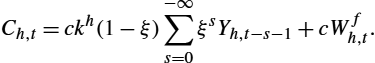
In words, consumption is a linear function of past incomes and financial wealth.
In the CATS/ADG framework, human capital is defined by the following adaptive algorithm: Whh,t=ξWhh,t−1+(1−ξ)Yh,t![]() . By iterating, one gets Whh,t=(1−ξ)Yh,t+(1−ξ)∑−∞s=1ξsYh,t−s
. By iterating, one gets Whh,t=(1−ξ)Yh,t+(1−ξ)∑−∞s=1ξsYh,t−s![]() , i.e., human capital is a weighted average of current and past incomes.27 Substituting this definition into (6), the behavioral rule specializes to
, i.e., human capital is a weighted average of current and past incomes.27 Substituting this definition into (6), the behavioral rule specializes to
(9) Ch,t=ch(1−ξ)Yh,t+ch(1−ξ)−∞∑s=1ξsYh,t−s+cfWfh,t.
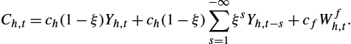
While human capital in the neoclassical approach is a linear combination of current and expected future incomes, and therefore is formed in a forward looking way, the proxy for human capital in AGH and CATS/ADG is a linear combination of current and past incomes, i.e., it is determined by a backward looking algorithm.28
Setting ξ=0![]() , i.e., assuming that there is no memory, human capital boils down to current income, so that (9) specializes to
, i.e., assuming that there is no memory, human capital boils down to current income, so that (9) specializes to
(10) Ch,t=cyYh,t+cfWfh,t
where cy![]() is the propensity to consume out of income.29
is the propensity to consume out of income.29
Setting cf=0![]() , from (10) we get a specification of the consumption function sometimes adopted in MABMs of a strictly Keynesian flavor
, from (10) we get a specification of the consumption function sometimes adopted in MABMs of a strictly Keynesian flavor
(11)
In many models of the KS family, the behavioral rule is (11) with ![]() :
:
(12)
This specification describes the behavior of “hand-to-mouth” consumers.30
LAGOM adopts a rule such as (10) with ![]() . Moreover, since financial wealth coincides with money holding (
. Moreover, since financial wealth coincides with money holding (![]() ), the consumption budget turns out to be an increasing linear function of real money balances31
), the consumption budget turns out to be an increasing linear function of real money balances31
(13)
In CATS/DD, consumption is a special case of (10) obtained by setting ![]() . Therefore
. Therefore
(14)
The expression in parentheses is one of the possible specifications of “cash-on-hand”, which can be defined in the most general way as liquid assets which can be used to carry on transactions. In small MABMs which do not feature banks such as LEN, cash-on-hand coincides with currency. In a setting with banks such as CATS/DD, cash-on-hand coincides with new deposits, which in turn amount to the sum of income and old deposits. This is in line with Deaton (1991), who defines cash-on-hand as the sum of income and financial assets.
In EUBI and EUGE, saving behavior aims at achieving a target for wealth, namely ![]() where
where ![]() is the target wealth-to-income ratio and ν is the velocity of adjustment of wealth to targeted wealth. Since by definition
is the target wealth-to-income ratio and ν is the velocity of adjustment of wealth to targeted wealth. Since by definition ![]() , simple algebra shows that under this assumption the consumption budget can be written as
, simple algebra shows that under this assumption the consumption budget can be written as
(15)
which is a special case of (10) with ![]() and
and ![]() .
.
Carroll has shown that in an uncertain world consumption is a concave function of cash-on-hand which he defines as the sum of human capital and beginning of period wealth.32 In Carroll's framework, for low values of wealth, the propensity to consume (out of wealth) is high due to the precautionary motive: a reduction of wealth would in fact lead to a sizable reduction of consumption to rebuild wealth (buffer stock rule). In some MABMs the consumption function is adjusted to mimic Carroll's precautionary motive, i.e., to reproduce the nonlinearity of the relationship between consumption and wealth. This theoretical setting has been corroborated by a number of empirical studies (see Carroll and Summers, 1991; Carroll, 1997), such that using this approach in MABMs is consistent with the agenda to rely on behavioral rules which have strong empirical foundations.
For instance, in EUBI the specification of the consumption function discussed above gives rise to a piecewise linear heuristic based on the buffer-stock rule. Also EUGE adopt a specification of the consumption budget which adopts Carroll's rule.
In the CATS/MBU framework, consumption is specified as in (11) but ![]() is a nonlinear function of wealth. This allows capturing the interaction between income and wealth in the determination of consumption.
is a nonlinear function of wealth. This allows capturing the interaction between income and wealth in the determination of consumption.
LEN explicitly models the consumption budget as an increasing concave function of money holdings by
(16)
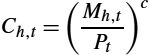
where ![]() .33
.33
JAMEL presents a variant of Carroll's framework. The household computes “average income” (which can be considered a proxy of permanent income) as the mean of incomes received over a certain time span occurred in the past, ![]() .34 Moreover, JAMEL define desired or targeted cash on hand as a fraction of average income,
.34 Moreover, JAMEL define desired or targeted cash on hand as a fraction of average income, ![]() , where
, where ![]() are real money balances and
are real money balances and ![]() is the desired propensity to save (out of average income). The consumption budget is defined as follows:
is the desired propensity to save (out of average income). The consumption budget is defined as follows:
(17)
where ![]() and
and ![]() is the propensity to consume. In words, if liquid assets are (relatively) “low”, the household spends a fraction c of average income. If liquidity is “high”, the household consumes the entire average income and a fraction
is the propensity to consume. In words, if liquid assets are (relatively) “low”, the household spends a fraction c of average income. If liquidity is “high”, the household consumes the entire average income and a fraction ![]() of excess money balances, defined as the difference between the current and targeted money holding.
of excess money balances, defined as the difference between the current and targeted money holding.
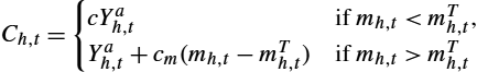
With the help of some algebra, the behavioral rule above can be written as follows:
(18)

where ![]() is the cut-off value of average income and
is the cut-off value of average income and ![]() . Notice that
. Notice that ![]() . The cut-off value of average income is a multiple of current money holdings. The specification above highlights the basic tenets of Carroll's buffer stock theory in a very simple piecewise linear setting. When average income is below the threshold, i.e., when the threshold is relatively high because the household is wealthy/liquid, the marginal propensity to consume is
. The cut-off value of average income is a multiple of current money holdings. The specification above highlights the basic tenets of Carroll's buffer stock theory in a very simple piecewise linear setting. When average income is below the threshold, i.e., when the threshold is relatively high because the household is wealthy/liquid, the marginal propensity to consume is ![]() , i.e., it is relatively high. When average income surpasses the threshold, the marginal propensity drops to c.
, i.e., it is relatively high. When average income surpasses the threshold, the marginal propensity drops to c.
JAMEL also incorporates consumer sentiment and opinion dynamics in the consumption function. The propensity to save, s, can take on two values. When “optimistic”, the household is characterized by ![]() while if “pessimistic” it sets s to
while if “pessimistic” it sets s to ![]() , with
, with ![]() . Pessimism leads to a reduction of the propensity to consume: households save more for rainy days.
. Pessimism leads to a reduction of the propensity to consume: households save more for rainy days.
Each household switches from a low to a high propensity to save (and vice versa) depending on its employment status. The household turns pessimistic if unemployed. In each period, the household observes the consumer sentiment (proxied by the employment status) of a finite subset of other households (a neighborhood, for short). With probability ![]() it adopts the majority opinion, i.e., the prevailing consumer sentiment, of the neighborhood; with probability
it adopts the majority opinion, i.e., the prevailing consumer sentiment, of the neighborhood; with probability ![]() the household relies on its own situation: if it is unemployed (employed), it will be pessimistic (optimistic) and will choose
the household relies on its own situation: if it is unemployed (employed), it will be pessimistic (optimistic) and will choose ![]() (
(![]() ). The probability of adopting the sentiment of the majority can be interpreted as the strength of the households' “animal spirits.”
). The probability of adopting the sentiment of the majority can be interpreted as the strength of the households' “animal spirits.”
The Choice of the Goods to Buy
As to the second stage, the choice of the goods to buy is generally influenced by the relative price. EUBI and EUGE introduce a multinomial logit model, CATS posit a search mechanism.
In LEN each household is linked to a fixed number of firms from which it can buy. The network can change over time. Each period, with a certain probability, the household chooses at random a firm in the neighborhood of current trading partners and a firm outside it, compares the prices, and switches to the new firm if the price of the price set by the current partner exceeds the price of the new firm by at least a certain margin. In the end, therefore, the household searches for better trading opportunities based on relative price.35
AGH posit that the household can buy only from two firms (“stores”, i.e., shops where the household purchases its consumption goods). Hence it has to choose the quantity to be demanded from each firm. AGH derives behavioral rules by solving a simple optimization problem. The household maximizes ![]() subject to
subject to ![]() where
where ![]() ,
, ![]() . Hence the quantity demanded for each variety turns out to be
. Hence the quantity demanded for each variety turns out to be
(19)
which can be easily compared with (22). The household explores the goods market looking for stores supplying the goods it wants to consume. The household buys from store j only if the posted price ![]() is smaller than a reservation price equal to the price paid by the household in the past
is smaller than a reservation price equal to the price paid by the household in the past ![]() (appropriately indexed):
(appropriately indexed): ![]() where
where ![]() is expected inflation, anchored to the inflation target of the central bank.36
is expected inflation, anchored to the inflation target of the central bank.36
In the CATS framework, households collect information and pick goods by visiting firms chosen at random. The hth household visits ![]() randomly selected firms, ranks them according to the price they charge and purchases C-goods starting from the firm charging the lowest price. If it does not spend the entire consumption budget at the first firm, it will move up to the second firm in the ranking, and so on. If it has not spent all the consumption budget after visiting
randomly selected firms, ranks them according to the price they charge and purchases C-goods starting from the firm charging the lowest price. If it does not spend the entire consumption budget at the first firm, it will move up to the second firm in the ranking, and so on. If it has not spent all the consumption budget after visiting ![]() firms, it will save involuntarily. This implies that the demand for the good produced by the ith C-firm is implicitly decreasing with the relative price
firms, it will save involuntarily. This implies that the demand for the good produced by the ith C-firm is implicitly decreasing with the relative price ![]() . Notice, however, that the implicit demand curve that the ith firm is facing is shifting over time. A given firm may be visited by different sets of consumers on subsequent days. The search and matching mechanism leads to the coexistence of queues of unsatisfied consumers (involuntary savers) at some firms and involuntary inventories of unsold goods at some other firms.
. Notice, however, that the implicit demand curve that the ith firm is facing is shifting over time. A given firm may be visited by different sets of consumers on subsequent days. The search and matching mechanism leads to the coexistence of queues of unsatisfied consumers (involuntary savers) at some firms and involuntary inventories of unsold goods at some other firms.
LAGOM adopts a similar market protocol as CATS for the market for C-goods. In the LAGOM model also firms enter the market for C-goods as they use circulating capital together with fixed capital for production.
EUBI and EUGE assume that the consumer receives information about the range of products, their prices, and their availability at (local) malls. The choice of the good to buy is random and the probability of buying a certain product is determined by a multinomial logit model:
(20)
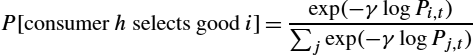
where the sum in the denominator includes all products for which the consumer has received information.37 As has been discussed in Dawid et al. (2018d), this formulation can also be interpreted as a representation of a situation in which the product offered by the different C-firms are horizontally differentiated along dimensions not explicitly captured in the model. The parameter γ governs the intensity of (price) competition between the C-firms and typically has strong influence on the emerging economic dynamics on the aggregate level. Dawid et al. (2018d) also point out that the use of logit-choice models for the representation of consumer choice has strong empirical foundations, e.g., in the Marketing literature.38
2.3.2 Labor Supply
On the labor market, households are suppliers of labor. The hth worker supplies inelastically one unit of labor.
LEN assumes that each household has a reservation wage, denoted with ![]() . It supplies its labor only to a finite subset of the population of firms, a neighborhood of potential employers. However, the network can be rewired. If the household is employed, say, at firm i, and its current wage is higher than the reservation wage (
. It supplies its labor only to a finite subset of the population of firms, a neighborhood of potential employers. However, the network can be rewired. If the household is employed, say, at firm i, and its current wage is higher than the reservation wage (![]() ), it will search for a better position infrequently, i.e., with probability less than one. When searching, it will visit only one new firm chosen at random. If at this new firm, say j, it finds
), it will search for a better position infrequently, i.e., with probability less than one. When searching, it will visit only one new firm chosen at random. If at this new firm, say j, it finds ![]() , so it will quit the current job and move to the jth firm. If, for any reasons, its current wage falls below the reservation wage (
, so it will quit the current job and move to the jth firm. If, for any reasons, its current wage falls below the reservation wage (![]() ),39 it will intensify the quest for a better position by exploring a new firm every period (i.e., with certainty). If the household is unemployed, it will search for a job every period by visiting a fixed number
),39 it will intensify the quest for a better position by exploring a new firm every period (i.e., with certainty). If the household is unemployed, it will search for a job every period by visiting a fixed number ![]() of firms chosen at random. If the household switches to a new employer, the former employer drops out of the set of employers of the households and is replaced by the new one.
of firms chosen at random. If the household switches to a new employer, the former employer drops out of the set of employers of the households and is replaced by the new one.
Also in LAGOM each household has a reservation wage. If the household is employed, say, at firm i, and its current wage is lower than the reservation wage (![]() ), so it will quit the job and search for a better position at a finite set of firms chosen at random.
), so it will quit the job and search for a better position at a finite set of firms chosen at random.
In AGH, as we saw above, a household type is defined by the production good it can produce with its labor type. If employed, the household is working in the same firm which produces its production good. If unemployed, the household engages in job search with a given probability ![]() . It explores the labor market looking for a firm (with the same product type) posting a vacancy. The household accepts the job offer if the previous wage
. It explores the labor market looking for a firm (with the same product type) posting a vacancy. The household accepts the job offer if the previous wage ![]() (appropriately indexed) is smaller than the posted wage
(appropriately indexed) is smaller than the posted wage ![]() , i.e., if
, i.e., if ![]() .
.
In CATS/MBU and CATS/ADG, the hth household, if unemployed, looks for a job by visiting ![]() firms chosen at random and applying to those with open vacancies. In CATS/MBU the posted wage is firm-specific and cannot drop below a lower bound represented by a minimum wage, which is changing over time due to indexation. The unemployed worker will accept a job from the firm with open vacancies which pays the highest wage. For simplicity in CATS/ADG the posted wage is given and is uniform across firms so that the unemployed worker accepts the job at the first chance of finding an open vacancy. If it doesn't find an open vacancy, the household remains unemployed and funds consumption by dissaving, i.e., consuming out of accumulated wealth. For simplicity CATS assume that there are neither hiring nor firing costs. If a firm wants to scale down activity in a certain period, it can fire workers at no cost. Fired workers become unemployed and start searching for a job in the same period.
firms chosen at random and applying to those with open vacancies. In CATS/MBU the posted wage is firm-specific and cannot drop below a lower bound represented by a minimum wage, which is changing over time due to indexation. The unemployed worker will accept a job from the firm with open vacancies which pays the highest wage. For simplicity in CATS/ADG the posted wage is given and is uniform across firms so that the unemployed worker accepts the job at the first chance of finding an open vacancy. If it doesn't find an open vacancy, the household remains unemployed and funds consumption by dissaving, i.e., consuming out of accumulated wealth. For simplicity CATS assume that there are neither hiring nor firing costs. If a firm wants to scale down activity in a certain period, it can fire workers at no cost. Fired workers become unemployed and start searching for a job in the same period.
In EUBI the household is characterized by a specific skill and has a reservation wage. If unemployed, it explores the labor market with a given probability. Firms post vacancies and wages. The unemployed household ranks the wage offers and applies only to firms that make a wage offer (for the worker's skill group) which is higher than its reservation wage. If the unemployed job searcher receives several acceptable job offers he/she accepts the offer with the highest wage. The reservation wage of the worker is adjusted downwards during periods of unemployment.
In JAMEL the household's reservation wage is stochastically reduced if the unemployment spell is greater than an exogenous upper bound. In symbols,
(21)

where ![]() is a random draw from a uniform distribution,
is a random draw from a uniform distribution, ![]() is the duration of the unemployment spell and
is the duration of the unemployment spell and ![]() is the threshold value of this spell.
is the threshold value of this spell.
2.3.3 The Demand for Financial Assets
In a small MABM such as LEN, households can hold wealth only in the most liquid form (cash). Most medium-sized MABMs assume that there is at least one other financial asset such as deposits at banks. For CATS, KS, JAMEL, and LAGOM, households' wealth consists only of deposits. In AGH, households can hold cash, deposits, and government bonds. In EUBI and EUGE the household can hold wealth as liquidity (deposits at banks), as a portfolio of shares issued by firms and banks, and in EUGE also as government bonds. Households therefore receive dividends according to the composition of their portfolio of shares. For simplicity, in EUBI the allocation of households' savings to bank deposits and shares is random. Modeling the portfolio choice for each household, however, may be quite complex. For instance, the preference structure of “investors” in EUGE, i.e., households trading in financial markets, takes into account insights from behavioral finance, namely myopic loss aversion. Transactions on financial markets occur at higher frequency than on real markets (daily as against monthly). Prices are determined in equilibrium through a clearinghouse mechanism. In CATS households can be of two types, workers and capitalists. Assuming that there is one capitalist per firm, each firm distributes part of its profits to the firm owner as dividends. KS adopt the extreme assumption that all the profits are retained within the firm and used to accumulate net worth. In this case, by assumption there will be no dividends. In JAMEL some households (chosen at random) are firm owners and therefore receive dividends which will be distributed only if the firm's net worth is higher than a threshold (defined by a target level for leverage). Opinion dynamics play a role in dividend distribution. Firms switch from “optimistic” (characterized by high target leverage and high dividends) to “pessimistic” (low target leverage and low dividends). Also in LAGOM households are firm owners and receive both wages and dividends.
2.4 Firms
In this section we will consider a population of F firms, which produce either consumption goods (C-firms) or capital goods (K-firms). Variables pertaining to the ith C-firm will be denoted with the index ![]() . Variables pertaining to the kth K-firm will be denoted with the index
. Variables pertaining to the kth K-firm will be denoted with the index ![]() . In most MABMs, C-firms demand labor and K-goods in order to produce and sell C-goods to households; K-firms demand labor in order to produce and sell K-goods to C-firms.40
. In most MABMs, C-firms demand labor and K-goods in order to produce and sell C-goods to households; K-firms demand labor in order to produce and sell K-goods to C-firms.40
Firms have market power, hence they set the quantity and the price of the goods they produce and sell. Generally, market power is rooted in transaction costs. Due to uncertainty and the costs of exploring market conditions, in fact, buyers do not have enough information on the prices and quantities set by all the sellers so that they purchase goods from a limited set of suppliers. Each supplier, therefore, operates in condition of monopolistic competition or oligopoly on the market for its own good.
The planned (or desired) scale of activity is the main determinant of the demand for inputs, namely the demand for capital and the demand for labor.
On the market for K-goods, demand comes from C-firms and supply comes from K-firms. The ith C-firm's demand for K-goods, i.e. investment, is driven mainly by production requirements. If production planned at period t for period ![]() can be carried out with the capital stock inherited from the past (after depreciation), the firm simply adjusts capacity utilization. If capital inherited from the past is insufficient to undertake planned production, the ith firm should expand capacity by purchasing new K-goods (sometimes referred to as “machine tools”). In some MABMs, this is feasible. In other MABMs, investment at period t is driven by long-run production requirements and cannot be used to face short-run peaks of demand. Hence the firm will be constrained to produce at full capacity but less than desired.
can be carried out with the capital stock inherited from the past (after depreciation), the firm simply adjusts capacity utilization. If capital inherited from the past is insufficient to undertake planned production, the ith firm should expand capacity by purchasing new K-goods (sometimes referred to as “machine tools”). In some MABMs, this is feasible. In other MABMs, investment at period t is driven by long-run production requirements and cannot be used to face short-run peaks of demand. Hence the firm will be constrained to produce at full capacity but less than desired.
On the market for labor, demand comes from all the firms and supply comes from households. Firms whose workforce is insufficient to undertake planned production will post vacancies and a wage offer (which may be firm-specific or uniform across firms, constant or time-varying because of indexation and/or because of labor market conditions.)
Firms may have a financing gap, i.e., a positive difference between operating costs and internally generated funds. They generally ask for a loan to fill this gap. The quantity and price of credit are set by banks.
Firms may be unable to achieve the desired scale of activity for lack of funds (if they are rationed on the credit market), of capital (if investment is disconnected from short-run production need and/or if they don't find enough machine tools to buy) or of labor (if they don't find enough workers to hire).
2.4.1 The Supply of Consumption Goods
The Dixit–Stiglitz Benchmark
As far as the corporate sector is concerned, NK DSGE models are based on monopolistic competition: each firm behaves as a monopolist on its own market. The firm's market power is due to product heterogeneity. Products may be different in the eyes of consumers for a number of reasons: spatial dispersion, product differentiation, or transaction costs which may generate captive markets.
In the Dixit–Stiglitz benchmark, the demand of the hth household for the ith good is represented by Eq. (5). Summing across H households and rearranging, one gets the demand function for the ith good:
(22)

where ![]() is total consumption (economywide).41
is total consumption (economywide).41
With a linear technology and only the labor input, the marginal cost will be ![]() where
where ![]() is the wage and α is the marginal productivity of labor. Optimal pricing yields
is the wage and α is the marginal productivity of labor. Optimal pricing yields
(23)
where ![]() is the mark-up.
is the mark-up.
Substituting (23) into (22), one gets the optimal scale of production
(24)
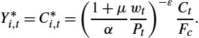
Since the manager of the firm knows the production function and input costs, and therefore can compute the marginal cost, if she knows also the demand curve she will choose an optimal mark-up (i.e., ratio of the individual price to marginal cost) and an optimal scale of activity. In other words, in the absence of uncertainty on market demand, the firm will choose a point on the demand curve in such a way as to maximize profits. In this case supply will always be equal to demand: the firm will neither accumulate involuntary inventories of unsold goods nor face queues of unsatisfied consumers; output will always be sold and no potential customer will leave the firm's premises empty handed.
Moreover, in the absence of frictions on the labor market, the firm will always be able to carry out planned production. In the end therefore, planned output will be equal to actual output and actual output will be equal to sales.
From (23) and (24) we can predict the following: the firm will react to (i) an increase of elasticity of demand by reducing the mark up and therefore the individual price and increasing production; (ii) an increase of the real wage by increasing the price and reducing production; (iii) an increase in productivity by reducing the price and increasing production; (iv) an increase in total consumption by increasing production.
Since firms have the same technology, incur the same labor cost, and face the same demand function, a symmetric equilibrium in which all firms charge the same price, is considered: ![]() , so that the real wage will be equal to
, so that the real wage will be equal to ![]() . At that wage, employment is determined by labor supply, the labor market clears, and there is full employment.42 Total output is equal to the full employment level of GDP.43 In the absence of investment, output is equal to consumption. Each firm therefore will produce the same quantity, i.e., a fraction
. At that wage, employment is determined by labor supply, the labor market clears, and there is full employment.42 Total output is equal to the full employment level of GDP.43 In the absence of investment, output is equal to consumption. Each firm therefore will produce the same quantity, i.e., a fraction ![]() of total consumption, which is equal to total full employment output. In the presence of nominal rigidities (e.g., Calvo pricing), this level of output is unattainable, at least in the short run.
of total consumption, which is equal to total full employment output. In the presence of nominal rigidities (e.g., Calvo pricing), this level of output is unattainable, at least in the short run.
Price/Quantity Decisions when Demand Is Unknown
In order to understand the price/quantity strategies of firms in MABMs and compare them with firms' decisions in the standard model, in this “intermezzo” we will keep the basic structure of the Dixit–Stiglitz framework, but will relax the assumption of perfect information as far as market demand is concerned. We will assume instead that, at the moment decisions on price and quantity must be made, the firm does not know the position of the demand curve on the price/quantity space.
Uncertainty on market demand may be due to the fact that transactions do not occur at the same time on all markets. There is a sequence of events which take place at different times on different markets. For instance, we can envisage the following 4 steps: (1) At the beginning of period t (before the market for C-goods opens), the firm decides the price and the quantity. On the basis of the production plan, it decides whether to hire or fire workers. Suppose the workforce must be expanded to fulfill the production plan. (2) The firm enters the labor market by posting vacancies at a certain wage. These vacancies may or may not be filled depending on the number of matches between demand (job offers) and supply (unemployed workers) of labor. Suppose all the vacancies are filled. (3) The firm can therefore implement the desired production plan. (4) The quantity produced is then sold on the market of C-goods. Production must be decided in step (1) but actual demand will be revealed to the firm only in step (4).
The information set of the firm at the moment the scale of activity must be decided may contain precise information on the pricing behavior of competitors and the total number of firms but information may be incomplete and imperfect on the price elasticity of demand and/or total households' consumption. In order to maximize expected profits, the firm must estimate the elasticity of demand and total consumption planned by households. The market demand that the ith firm expects is
(25)
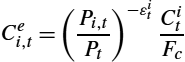
where ![]() and
and ![]() are price elasticity and total consumption expected or estimated by firm i. In order to maximize profits in this informational scenario, the firm could set the price as a mark up over marginal cost, the mark-up being a function of the estimated price elasticity:
are price elasticity and total consumption expected or estimated by firm i. In order to maximize profits in this informational scenario, the firm could set the price as a mark up over marginal cost, the mark-up being a function of the estimated price elasticity:
(26)
where ![]() . Plugging (26) into (25), one gets
. Plugging (26) into (25), one gets
(27)
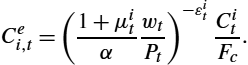
The firm uses expected demand to plan production, ![]() . For the sake of discussion, let's assume that actual production is equal to desired production,
. For the sake of discussion, let's assume that actual production is equal to desired production, ![]() . Hence44
. Hence44
(28)
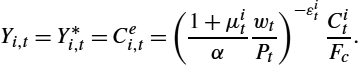
At the beginning of time t (step (1) in the sequence above) the status quo for the ith firm is the point ![]() on the price/quantity space. The coordinates are determined by (26) and (28). Once production has been carried out, transactions can take place. Once transactions are completed, the ith firm can observe the amount of goods actually sold
on the price/quantity space. The coordinates are determined by (26) and (28). Once production has been carried out, transactions can take place. Once transactions are completed, the ith firm can observe the amount of goods actually sold ![]() where
where ![]() is actual demand.
is actual demand.
Since sales occur only after the firm has carried out production, actual demand can differ from current production. If ![]() , there will be involuntary inventories whose size is
, there will be involuntary inventories whose size is ![]() . This is a signal of excess supply, i.e., of a positive forecasting error (demand has been overestimated).
. This is a signal of excess supply, i.e., of a positive forecasting error (demand has been overestimated).
If ![]() , all the output will be sold and therefore there will not be involuntary inventories,
, all the output will be sold and therefore there will not be involuntary inventories, ![]() . The difference
. The difference ![]() measures the demand of unsatisfied consumers, who may turn to other producers (goods are substitutable, albeit only imperfectly) or save involuntarily. This is a signal of excess demand. The firm has made a negative forecasting error (demand has been underestimated).
measures the demand of unsatisfied consumers, who may turn to other producers (goods are substitutable, albeit only imperfectly) or save involuntarily. This is a signal of excess demand. The firm has made a negative forecasting error (demand has been underestimated).
It can also happen, of course, that demand equals production, ![]() . There will be no forecasting error (no inventories and no queues) in this case.
. There will be no forecasting error (no inventories and no queues) in this case.
Inventories are defined as
(29)
In the case of excess demand or excess supply the firm is underperforming,45 and has an incentive to choose a different price/quantity in the future, say ![]() .
.
One possible strategy consists in setting the direction of the change in price and quantity in line with the sign of the forecasting error. For instance, if ![]() , the firm has an incentive to scale down production and cut the price. The size of the change may be linked to the magnitude of the error.
, the firm has an incentive to scale down production and cut the price. The size of the change may be linked to the magnitude of the error.
Notice that by making mistakes the firm collects new information on market conditions. As an alternative strategy, the firm can therefore make new estimates of demand and set the price and the quantity accordingly (see Eqs. (26) and (28)).
In the end, uncertainty and imperfect knowledge induce the firm to adapt period by period to evolving market conditions. This adaptation takes the form of price and quantity updating rules. There is no guarantee that this adaptation will lead to the type of equilibrium discussed above.
The Agent-Based Approach to Price/Quantity Decisions
The MABMs we are surveying generally conceive firms as production/trading units immersed in a market environment which is utterly uncertain. Uncertainty is due to the sequential nature of the market economy (which is easily replicated in an agent based framework) and to the ever changing conditions of demand and supply.
Different MABMs deal with price/quantity strategies in different ways. For most of the models we can detect a general pattern, however, in the description of the behavioral rules the firm adopts.46 The firm starts with an initial pair of price and quantity, (![]() ), which we define the status quo. At the end of period t, once transactions have been carried out, the firm observes actual sales
), which we define the status quo. At the end of period t, once transactions have been carried out, the firm observes actual sales ![]() and learns also the average price
and learns also the average price ![]() , which is a proxy of the price charged on average by the firms' competitors.
, which is a proxy of the price charged on average by the firms' competitors.
If ![]() , there will be an inventory equal to
, there will be an inventory equal to ![]() . Notice that the firm may want to hold a buffer stock of finished goods (desired or voluntary or target inventories). Desired inventories may be an interval,
. Notice that the firm may want to hold a buffer stock of finished goods (desired or voluntary or target inventories). Desired inventories may be an interval, ![]() , where the extremes are the minimum and maximum levels of desired inventories, or collapse to a single point,
, where the extremes are the minimum and maximum levels of desired inventories, or collapse to a single point, ![]() . In the first case there will be a shortage of inventories if
. In the first case there will be a shortage of inventories if ![]() and excess (or involuntary) inventories
and excess (or involuntary) inventories ![]() if
if ![]() . In the second case there will be a shortage of inventories (resp. involuntary inventories) if
. In the second case there will be a shortage of inventories (resp. involuntary inventories) if ![]() (resp.
(resp. ![]() ). It is reasonable to assume that planned production for period t will take into account expected demand in the same period and desired inventories.
). It is reasonable to assume that planned production for period t will take into account expected demand in the same period and desired inventories.
Of course, desired inventories may be zero, ![]() . In this case, planned production is equal to expected demand,
. In this case, planned production is equal to expected demand, ![]() , the difference
, the difference ![]() therefore is the forecasting error. A positive inventory will always be involuntary and coincide with the absolute value of the (negative) forecasting error,
therefore is the forecasting error. A positive inventory will always be involuntary and coincide with the absolute value of the (negative) forecasting error, ![]() and
and ![]() . If
. If ![]() , the forecasting error is positive (
, the forecasting error is positive (![]() ), there are no inventories (
), there are no inventories (![]() ) but a fringe of unsatisfied consumers.
) but a fringe of unsatisfied consumers.
Desired inventories are generally determined by applying a desired or target inventory-to-sales ratio ![]() to current production
to current production ![]() . This ratio represents the number of periods of production at the current rate necessary to build desired inventories. Hence the minimum and maximum levels of voluntary inventories are determined as follows:
. This ratio represents the number of periods of production at the current rate necessary to build desired inventories. Hence the minimum and maximum levels of voluntary inventories are determined as follows: ![]() and
and ![]() ,
, ![]() . The parameters
. The parameters ![]() and
and ![]() are the minimum and the maximum inventory-to-sales ratios. If there are no desired inventories, then
are the minimum and the maximum inventory-to-sales ratios. If there are no desired inventories, then ![]() .
.
The firm receives two types of signals of market conditions: (i) an excess or shortage of inventories (with respect to the target, which may be an interval, a positive value or zero); (ii) the relative price, i.e., the ratio or difference between the individual price and average price. From signals of type (i) the firm infers that it has underestimated or overestimated the strength of demand: a shortage of inventories reveals stronger than expected demand; an involuntary inventory signals weaker than expected demand. From signals of type (ii) the firm infers its position relative to competitors: if the firm's price is lower than the average price, the firm is undercutting competitors (and its market share is bigger than the average market share); if the opposite holds true, the good produced by the firm is overpriced with respect to competitors (and its market share is smaller than the average market share).47 The sign and size of signals determine the direction of the price and quantity change to be implemented. The magnitude of the price and quantity change is stochastic and/or governed by the signals. The change in price and quantity therefore will be governed by behavioral rules which take the form of updating algorithms.
The most general form of a quantity updating algorithm we can detect in the MABMs under scrutiny is
(30)

In words, the firm revises production plans up (resp. down) by ![]() if there is a shortage (resp. excess) of inventories and the current price is greater (resp. smaller) than the competitors' price. The assumption of an upper and a lower bound on the level of desired inventories introduces inertia in quantity updating: if actual inventories fall in the desired interval, the firm does not change the scale of activity.
if there is a shortage (resp. excess) of inventories and the current price is greater (resp. smaller) than the competitors' price. The assumption of an upper and a lower bound on the level of desired inventories introduces inertia in quantity updating: if actual inventories fall in the desired interval, the firm does not change the scale of activity.
The most general form of a price updating algorithm is
(31)
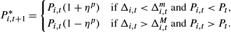
In words, the firm revises the price up (resp. down) by ![]() if there is a shortage (excess) of inventories and the current price is smaller (greater) than the competitors' price.
if there is a shortage (excess) of inventories and the current price is smaller (greater) than the competitors' price.
We will now survey the specifications of these general rules adopted in some of the MABMs under scrutiny. Let's start with a small MABM. LEN posits the following quantity updating rule:
(32)
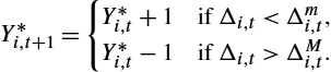
In words, the firm scales up production by one unit if inventories are “too low”, i.e., smaller than the minimum. On the other hand, the firm scales down production if inventories are “too high”, i.e., greater than the maximum. LEN assumes the firm has a one-to-one technology which uses only labor as input, ![]() . Therefore, in order to scale up production by one unit, the firm has to post a vacancy. The firm scales down production by one unit by firing a worker chosen at random in the employed workforce.48
. Therefore, in order to scale up production by one unit, the firm has to post a vacancy. The firm scales down production by one unit by firing a worker chosen at random in the employed workforce.48
The rule (32) is a special case of (30), in which the signal coming from the relative price is ignored. Moreover, the change in quantity is a discrete step of size one.
As to pricing, LEN assumes that the firm wants the actual mark-up ![]() to fall into a prespecified interval
to fall into a prespecified interval ![]() where
where ![]() . The introduction of an upper and a lower bound on mark-ups mitigates price volatility. In fact, the current price is deemed adequate if
. The introduction of an upper and a lower bound on mark-ups mitigates price volatility. In fact, the current price is deemed adequate if ![]() where
where ![]() and
and ![]() are the minimum and maximum prices. LEN posits the following price updating rule:
are the minimum and maximum prices. LEN posits the following price updating rule:
(33)

where ![]() is a random draw from a uniform distribution. In words, the firm raises the posted price if inventories are “too low” provided the current price is smaller than the maximum. On the other hand, the firm cuts the price if inventories are “too high” provided the current price is higher than the minimum. The size of the rate of change is stochastic.
is a random draw from a uniform distribution. In words, the firm raises the posted price if inventories are “too low” provided the current price is smaller than the maximum. On the other hand, the firm cuts the price if inventories are “too high” provided the current price is higher than the minimum. The size of the rate of change is stochastic.
LEN introduces inertia in price changes which may result in stickiness. In fact, there is an interval of values for inventories such that the firm does not change the price.49
Expression (33) is a special case of (31), in which the signal coming from the relative price has been replaced by an upper and lower bound on the range of the mark-up (with no reference to the prices charged by the competitors).
In AGH, before deciding to enter the market and produce, the firm conducts market research by sending out a message to people who are prospective buyers. This message contains the “normal” posted price ![]() where
where ![]() is the posted wage.50 The mark-up μ is drawn from a uniform distribution.
is the posted wage.50 The mark-up μ is drawn from a uniform distribution.
As in LEN, AGH assume that the firm wants to keep a buffer stock of finished goods. Contrary to LEN, however, the desired size of inventories is unique, ![]() . AGH assume a fairly simple price updating rule:
. AGH assume a fairly simple price updating rule:
(34)
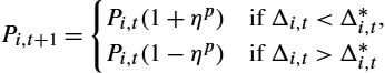
where ![]() is a random draw from a uniform distribution. Rule (34) is a special case of (31), in which
is a random draw from a uniform distribution. Rule (34) is a special case of (31), in which ![]() and the relative price has no role to play.
and the relative price has no role to play.
The prospective customer (household h) decides to buy if the price posted by firm i is smaller than the price the household previously paid – by purchasing goods at firm j – updated by means of expected inflation, equal to the inflation target of the central bank. In symbols, ![]() .
.
Transactions occur in the following way. The household visits two stores, 1 and 2. Consider one of the two, say, store 1, which has inventories ![]() . The household can place an order for
. The household can place an order for ![]() 51 if a cash-in-advance constraint is satisfied,
51 if a cash-in-advance constraint is satisfied, ![]() where
where ![]() are the household's money holdings. The store offers an amount
are the household's money holdings. The store offers an amount ![]() . Suppose the household previously purchased goods at firm 2. The households decides to buy from firm 1 if
. Suppose the household previously purchased goods at firm 2. The households decides to buy from firm 1 if ![]() .
.
Upon entering the market, according to AGH, the firm sets a target for the labor input ![]() , which must satisfy the requirement to produce desired output
, which must satisfy the requirement to produce desired output ![]() , given the fixed labor input (overhead costs) F and the need to move closer to desired inventories:
, given the fixed labor input (overhead costs) F and the need to move closer to desired inventories:
(35)
where ![]() is the inventory adjustment speed.
is the inventory adjustment speed.
In CATS, firms explore the price-quantity space around their status quo ![]() in order to maximize profits by adapting to the market environment. For simplicity, in this overview of firms' behavior in CATS, we will assume that planned production can be always carried out,
in order to maximize profits by adapting to the market environment. For simplicity, in this overview of firms' behavior in CATS, we will assume that planned production can be always carried out, ![]() .52 Notice that desired inventories are zero in this setting, i.e.,
.52 Notice that desired inventories are zero in this setting, i.e., ![]() .
.
Once transactions have been carried out, the information set of the firm ![]() consists of two signals: the average price
consists of two signals: the average price ![]() and the forecasting error
and the forecasting error ![]() . These signals capture – albeit imprecisely – the distance between the firm's actual position (the status quo) and the “benchmark”, i.e., a situation in which all firms charge the same price and demand equals supply:
. These signals capture – albeit imprecisely – the distance between the firm's actual position (the status quo) and the “benchmark”, i.e., a situation in which all firms charge the same price and demand equals supply: ![]() and
and ![]() .53 There are four cases: (a)
.53 There are four cases: (a) ![]() ; (b)
; (b) ![]() ; (c)
; (c) ![]() ; (d)
; (d) ![]() . On the basis of this information, the firm decides (i) whether to change the price or the quantity in period
. On the basis of this information, the firm decides (i) whether to change the price or the quantity in period ![]() (with respect to the status quo in period t), (ii) in which direction, and (iii) the size of such a change.
(with respect to the status quo in period t), (ii) in which direction, and (iii) the size of such a change.
As to quantity, the firm sets in period t desired production ![]() for period
for period ![]() at the level of expected future demand, i.e.,
at the level of expected future demand, i.e., ![]() . Expectations of future demand are based on the forecasting error
. Expectations of future demand are based on the forecasting error ![]() . CATS/ADG assume that the firm decides to update the desired scale of activity as follows:
. CATS/ADG assume that the firm decides to update the desired scale of activity as follows:
(36)
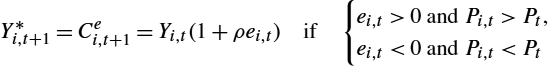
where ![]() . The firm revises expected demand (and desired production) up if there is a queue of unsatisfied consumers (
. The firm revises expected demand (and desired production) up if there is a queue of unsatisfied consumers (![]() ) and the price is higher than the average price (case (a)). The change in the scale of activity is proportional to the size of the error. If the firm's price is smaller than the average price, the firm does not adjust production even in the presence of a queue (case (b)). As we will see below, in case (b) the firm will revise the price up.
) and the price is higher than the average price (case (a)). The change in the scale of activity is proportional to the size of the error. If the firm's price is smaller than the average price, the firm does not adjust production even in the presence of a queue (case (b)). As we will see below, in case (b) the firm will revise the price up.
The firm revises expected demand and desired production down if ![]() and the price is lower than the average price (case (d)). The decrease in activity in this case is proportional to the level of involuntary inventories,
and the price is lower than the average price (case (d)). The decrease in activity in this case is proportional to the level of involuntary inventories, ![]() . If
. If ![]() but the price is higher than the average price, on the contrary, the firm will cut the price, keeping the quantity constant (case (c)).
but the price is higher than the average price, on the contrary, the firm will cut the price, keeping the quantity constant (case (c)).
Expression (36) is a special case of (30) with ![]() in case of excess demand and
in case of excess demand and ![]() in case of excess supply.
in case of excess supply.
This updating rule is based implicitly on an adaptive scheme to compute expected future demand, ![]() . Recalling that
. Recalling that ![]() , by iterating, it is easy to see that expected future demand is a weighted average of current and past demand with exponentially decaying weights:
, by iterating, it is easy to see that expected future demand is a weighted average of current and past demand with exponentially decaying weights:
(37)

As to the price, CATS/ADG assume the following updating rule:
(38)
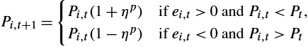
where ![]() is drawn from a uniform distribution. The firm revises the price up if there is a queue of unsatisfied consumers and the price is lower than the average price (case (b)): an increase of the price will mitigate excess demand for the good in question. If the firm's price is higher than the average price, in the presence of a queue the firm adjusts not the price but quantity (case (a)).
is drawn from a uniform distribution. The firm revises the price up if there is a queue of unsatisfied consumers and the price is lower than the average price (case (b)): an increase of the price will mitigate excess demand for the good in question. If the firm's price is higher than the average price, in the presence of a queue the firm adjusts not the price but quantity (case (a)).
It is easy to see that (38) is a special case of (31) with ![]() .
.
The firm revises the price down if there is an involuntary inventory and the price is higher than the average price (case (c)): a reduction of the price will boost demand (and will allow increasing the market share). If the firm's price is lower than the average price, in the presence of inventories the firm adjusts not the price but quantity (case (d)).
The mark-up therefore is determined residually by the joint dynamics of the price – governed by the stochastic adjustment mechanism described in (38) – and the average cost, which is determined endogenously.
It is worth noting that once the direction of the price change has been decided on the basis of the signals, the size of the price change is determined by a random draw. Contrary to the updating rule for the quantity, in the updating rule for the price the size of the adjustment does not depend on the size of the error. In CATS/MBU, there is symmetry in the updating rules because the sizes of both the price and quantity adjustments are stochastic.
In this MABM an (unexpected) upward shift of the demand function (due, for instance, to an increase of total output, which will boost the consumption budget of each and every household) will create a queue and bring about an increase of production if the price is above the average price (case (a)); an increase of the price if the latter is below the average price (case (b)).
Financial factors seem to play no role in the price and quantity decisions of firms. This is not true. First, CATS assume there is a lower bound of the firm's price: the firm will never set the price below the average cost, which consists of operating costs (incurred to hire workers and purchase capital goods) and debt commitments. If interest payments increase, the average cost goes up and this may affect price and quantity decisions.
Second, once the scale of production has been decided, the firm goes to the bank asking for a loan to fill the financing gap (see below, Section 2.4.5). But the bank may refuse to extend a loan of the requested size. In this case the firm is rationed and has to scale down production. In other words, the firm is subject to an ex post borrowing constraint.
In a couple of CATS models characterized by a network based financial accelerator, planned production is financially constrained ex ante. For instance, Riccetti et al. (2013, 2016b) assume that the firm takes explicitly into account its balance sheet in deciding production. The production function is ![]() where
where ![]() is the firm's capital stock and
is the firm's capital stock and ![]() . The firm sets a leverage target
. The firm sets a leverage target ![]() where leverage is defined as the ratio of debt (bank loans) to net worth.54 Hence the target level of debt is
where leverage is defined as the ratio of debt (bank loans) to net worth.54 Hence the target level of debt is ![]() where
where ![]() is net worth. Since
is net worth. Since ![]() by definition, it turns out that
by definition, it turns out that
(39)
In a previous model, Delli Gatti et al. (2010) posit a financially constrained output function ![]() which is a special case of Riccetti et al. (2013, 2016b).
which is a special case of Riccetti et al. (2013, 2016b).
In EUBI, following the “Management Science” approach, the procedure determining a firm's price and quantity is based on heuristics put forward in the literature on Operations Management and strategic pricing. A given firm (say firm i) in a given period ![]() knows the market size (total consumption expenditure) in the past n periods, i.e.,
knows the market size (total consumption expenditure) in the past n periods, i.e., ![]() for
for ![]() . This means that the firm has a time series of aggregate consumption consisting of n data points. The firm estimates total consumption by simple linear regression, the regressor being time:
. This means that the firm has a time series of aggregate consumption consisting of n data points. The firm estimates total consumption by simple linear regression, the regressor being time: ![]() where
where ![]() and
and ![]() are the estimated intercept and slope of the regression line. Hence the estimated current market size will be
are the estimated intercept and slope of the regression line. Hence the estimated current market size will be ![]() and the future market size at time
and the future market size at time ![]() can be estimated as follows:
can be estimated as follows: ![]() . From this simple statistical exercise, the firm derives a way of updating expectations of aggregate demand for C-goods.
. From this simple statistical exercise, the firm derives a way of updating expectations of aggregate demand for C-goods.
Then the firm adopts a market research procedure to estimate the distribution of demand ![]() for different own price levels given the price of competitors. The firm conducts a survey on a sample of consumers55 asking whether they would buy product i at Z different prices
for different own price levels given the price of competitors. The firm conducts a survey on a sample of consumers55 asking whether they would buy product i at Z different prices ![]() ,
, ![]() , given the prices of the
, given the prices of the ![]() competitors,
competitors, ![]() ,
, ![]() . This survey will determine a discrete distribution: each of the Z prices will be associated with the fraction of sampled households who would buy the product at that price, say,
. This survey will determine a discrete distribution: each of the Z prices will be associated with the fraction of sampled households who would buy the product at that price, say, ![]() . In this way, the firm determines a cross-section of Z data points, (
. In this way, the firm determines a cross-section of Z data points, (![]() ),
), ![]() .56
.56
Using the Z data points, the firm performs a regression of the fraction of buying households on the price according to the following specification: ![]() where
where ![]() and
and ![]() are estimated parameters.57 Current expected demand is
are estimated parameters.57 Current expected demand is ![]() where
where ![]() .
.
EUBI assume that the firm adopts an autoregressive model to estimate the future value of the fraction. Therefore the demand curve in period ![]() estimated by the firm using data available up to
estimated by the firm using data available up to ![]() will be
will be ![]() where
where ![]() .
.
The firm then uses this estimates to determine its expected profit over a given planning horizon for each price and chooses the price which maximizes this profit.58 The pricing procedure adopted in EUBI essentially leads to mark-ups determined by the estimated price elasticity of the firm's demand and therefore is well in accordance with standard results on optimal pricing discussed in the beginning of this subsection.
Since demand is uncertain and the firm may incur “stock-out costs” because consumers will switch to competitors if the firm's inventory at a mall is empty, the firm estimates the volatility of demand (standard deviation of the demand distribution denoted by ![]() ) and uses this estimate to determine a desired buffer stock.59 Production therefore must satisfy expected demand for the chosen price and generate a desired inventory:
) and uses this estimate to determine a desired buffer stock.59 Production therefore must satisfy expected demand for the chosen price and generate a desired inventory:
(40)
where ![]() is the χ quantile of the standard normal distribution and
is the χ quantile of the standard normal distribution and ![]() are desired inventories.
are desired inventories.
In EUGE the firm estimates future demand using a linear regression on its own past sales. Given inventories, the firm sets the quantity to be produced as follows:
(41)
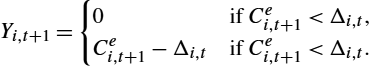
As to pricing, EUGE assume a standard mark up pricing rule
(42)
where μ is an exogenous mark up (uniform across firms) and ![]() is a weighted average of the unit cost of current production and past production stocked in inventories. Costs consist of the wage bill, interest payments, and the cost of capital depreciation.
is a weighted average of the unit cost of current production and past production stocked in inventories. Costs consist of the wage bill, interest payments, and the cost of capital depreciation.
In KS, the firm plans production in period t in such a way as to satisfy expected demand ![]() in period
in period ![]() and to generate the desired inventory:
and to generate the desired inventory:
(43)
The expectation of future demand ![]() is generated by past demand on the basis of an adaptive rule such as (37).
is generated by past demand on the basis of an adaptive rule such as (37).
As to pricing, KS assume the following mark up pricing rule:
(44)
where ![]() represents unit labor cost;
represents unit labor cost; ![]() is labor productivity due to use in production of the machine tool purchased at the jth K-firm (see Section 2.4.2).
is labor productivity due to use in production of the machine tool purchased at the jth K-firm (see Section 2.4.2).
Whereas in the MABMs reviewed so far the mark-up is either fixed or determined implicitly by the choice of the price, given the average cost, KS posit an updating rule for the mark-up:
(45)
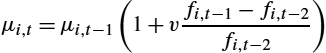
where v is a parameter and ![]() is the firm's market share. In words, the rate of change of the mark-up between
is the firm's market share. In words, the rate of change of the mark-up between ![]() and t is assumed to be proportional to the rate of change of the market share between
and t is assumed to be proportional to the rate of change of the market share between ![]() and
and ![]() .
.
The change in market share, in turn, is governed by the change in competitiveness ![]() according to a “quasi-replicator dynamics”:
according to a “quasi-replicator dynamics”:
(46)
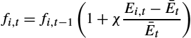
where ![]() is average competitiveness of C-firms. In words, the rate of change of the market share of firm i is proportional to relative competitiveness
is average competitiveness of C-firms. In words, the rate of change of the market share of firm i is proportional to relative competitiveness ![]() . If relative competitiveness is positive, i.e., if the ith firm is more competitive than the average, its share increases (and vice versa). In the evolutionary environment of KS models, relative competitiveness is a selection criterion as it governs industry dynamics, i.e., expansion, contraction, and extinction of firms.
. If relative competitiveness is positive, i.e., if the ith firm is more competitive than the average, its share increases (and vice versa). In the evolutionary environment of KS models, relative competitiveness is a selection criterion as it governs industry dynamics, i.e., expansion, contraction, and extinction of firms.
Finally, ![]() is defined as a decreasing function of the firm's price and of unfilled demand,
is defined as a decreasing function of the firm's price and of unfilled demand, ![]() . In fact, customers dissatisfied with a firm, which is unable to provide the goods they want to purchase, will switch to competitors. Since
. In fact, customers dissatisfied with a firm, which is unable to provide the goods they want to purchase, will switch to competitors. Since ![]() is a weighted average of the individual measures of competitiveness, it will be a linear function of the average price level
is a weighted average of the individual measures of competitiveness, it will be a linear function of the average price level ![]() and average unfilled demand. In the end therefore, the relative competitiveness of the ith firm is determined by the relative price
and average unfilled demand. In the end therefore, the relative competitiveness of the ith firm is determined by the relative price ![]() and the relative performance in fulfilling demand. It is worth noting, for comparison, that in the Dixit–Stiglitz benchmark, when prices are fully flexible, the mark-up is determined only by price elasticity. In the presence of nominal rigidities, the mark up is anticyclical: in a Calvo setting, when the firm is unable to change the price, a demand boost will make the mark-up shrink.
and the relative performance in fulfilling demand. It is worth noting, for comparison, that in the Dixit–Stiglitz benchmark, when prices are fully flexible, the mark-up is determined only by price elasticity. In the presence of nominal rigidities, the mark up is anticyclical: in a Calvo setting, when the firm is unable to change the price, a demand boost will make the mark-up shrink.
In JAMEL given the capital stock (see Section 2.4.2), ![]() is proportional to the stock of workers
is proportional to the stock of workers ![]() . Changes in production, therefore, require proportional changes in employment obtained by hiring/firing workers. JAMEL assume that there is a maximum level of inventories the firm can hold, which is proportional to the desired level of inventories. The desired level of inventories is
. Changes in production, therefore, require proportional changes in employment obtained by hiring/firing workers. JAMEL assume that there is a maximum level of inventories the firm can hold, which is proportional to the desired level of inventories. The desired level of inventories is ![]() . The maximum level of inventories is
. The maximum level of inventories is ![]() where
where ![]() is a random draw from a uniform distribution. Employment and output decisions are determined by the distance between actual inventories and the maximum level of inventories:
is a random draw from a uniform distribution. Employment and output decisions are determined by the distance between actual inventories and the maximum level of inventories:
(47)

where ![]() is a random draw from a uniform distribution. Pricing follows a similar updating rule, namely
is a random draw from a uniform distribution. Pricing follows a similar updating rule, namely
(48)
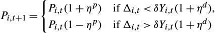
where ![]() is a random draw from a uniform distribution.
is a random draw from a uniform distribution.
In words, the firm scales up production (by posting vacancies) and increases the price if inventories are “too low”; it scales down production by firing workers and cuts the price if inventories are “too high”.60,61
If desired production is equal to expected demand, ![]() , and involuntary inventories are a symptom of a forecasting error, the quantity updating rule above can be reinterpreted as follows. The firm revises expected demand up (stochastically) if (i) it has underestimated demand (there are no inventories) or (ii) it has overestimated demand but “not too much”; the firm revises expected demand down if it has overestimated demand by a “large” margin.
, and involuntary inventories are a symptom of a forecasting error, the quantity updating rule above can be reinterpreted as follows. The firm revises expected demand up (stochastically) if (i) it has underestimated demand (there are no inventories) or (ii) it has overestimated demand but “not too much”; the firm revises expected demand down if it has overestimated demand by a “large” margin.
In LAGOM the firm is assumed to have a moving target for production:
(49)
where ![]() is increasing with all the arguments, except inventories. The price is updated using a similar algorithm.
is increasing with all the arguments, except inventories. The price is updated using a similar algorithm.
2.4.2 Technology
In LEN, production is carried out by means of a one-to-one technology which uses only labor. In AGH, capital plays a role only as collateral. Each household supplies one unit of labor of a specific type which is transformed through production in one unit of goods of the same type. The technology in some of the CATS models does not use capital (e.g., CATS/MBU) or does not use labor (Delli Gatti et al., 2005).
In this section we will refer to CATS/ADG as a benchmark CATS model with capital. In CATS/ADG the ith firm produces output ![]() by means of capital
by means of capital ![]() and labor
and labor ![]() . For simplicity ADG assume a Leontief technology. In a condition of full capacity utilization the output will be
. For simplicity ADG assume a Leontief technology. In a condition of full capacity utilization the output will be
(50)
where α and κ are the productivities of labor and capital, respectively, both exogenous, constant, and uniform across firms. Assuming that labor is always abundant, ![]() . Hence labor requirements at full capacity utilization is
. Hence labor requirements at full capacity utilization is ![]() , where
, where ![]() is the reciprocal of the (given and constant) capital/labor ratio. When capacity is not fully utilized, only a fraction
is the reciprocal of the (given and constant) capital/labor ratio. When capacity is not fully utilized, only a fraction ![]() of the capital stock will be used in production. Here
of the capital stock will be used in production. Here ![]() represents the rate of capacity utilization. In this context, the marginal cost of production is constant and independent of the scale of production,
represents the rate of capacity utilization. In this context, the marginal cost of production is constant and independent of the scale of production, ![]() .
.
JAMEL posits the same Leontief production function but assumes ![]() so that the capital/labor ratio is equal to one. Contrary to CATS/ADG, each firm has a given endowment of capital K (measured in numbers of identical machine tools) which does not depreciate and is not accumulated by means of investment. “Capital” therefore is a nonreproducible and durable input which is available in fixed supply, evenly spread across firms. Hence
so that the capital/labor ratio is equal to one. Contrary to CATS/ADG, each firm has a given endowment of capital K (measured in numbers of identical machine tools) which does not depreciate and is not accumulated by means of investment. “Capital” therefore is a nonreproducible and durable input which is available in fixed supply, evenly spread across firms. Hence ![]() and labor requirement is
and labor requirement is ![]() : each machine is operated by a worker. Production takes time. Each machine needs n periods to produce κ units of output. Output is added to inventories of finished goods. As we saw above, there is a desired level of inventories (identical for all firms) δκK where δ is the desired inventories-to-output ratio.
: each machine is operated by a worker. Production takes time. Each machine needs n periods to produce κ units of output. Output is added to inventories of finished goods. As we saw above, there is a desired level of inventories (identical for all firms) δκK where δ is the desired inventories-to-output ratio.
LAGOM posit a variant of (50), namely ![]() where
where ![]() is the firm's stock of circulating capital (e.g., raw materials) and
is the firm's stock of circulating capital (e.g., raw materials) and ![]() is the productivity of circulating capital. In the production process which takes place in one period, circulating capital is depleted completely while fixed capital and inventories of finished goods depreciate at a constant rate.
is the productivity of circulating capital. In the production process which takes place in one period, circulating capital is depleted completely while fixed capital and inventories of finished goods depreciate at a constant rate.
In EUBI, as well as in KS, capital goods (“machine tools”) are heterogeneous since different vintages of machine tools are characterized by different productivities. We will denote with ![]() the productivity of a machine tool of vintage v,
the productivity of a machine tool of vintage v, ![]() .
.
In KS K-firms develop new vintages over time by means of innovation and imitation. The probability for a K-firm to innovate or imitate ![]() with
with ![]() is assumed to be increasing with its R&D expenditure
is assumed to be increasing with its R&D expenditure ![]() :
:
(51)
where ![]() is the parameter characterizing the Bernoulli distribution. Notice that R&D expenditure, in turn, is proportional to past sales. Hence the probability to innovate/imitate is driven by high demand coming from C-firms, which in turn is high when households' demand for C-goods is high. The innovating K-firm draws a new machine embodying a technology inducing productivity
is the parameter characterizing the Bernoulli distribution. Notice that R&D expenditure, in turn, is proportional to past sales. Hence the probability to innovate/imitate is driven by high demand coming from C-firms, which in turn is high when households' demand for C-goods is high. The innovating K-firm draws a new machine embodying a technology inducing productivity ![]() given by
given by
(52)
where ![]() is drawn from a Beta distribution characterized by parameters
is drawn from a Beta distribution characterized by parameters ![]() . Changes in these parameters, and therefore in the shape of the distribution, capture technological opportunities for the economy under scrutiny.
. Changes in these parameters, and therefore in the shape of the distribution, capture technological opportunities for the economy under scrutiny.
In EUBI there is complementarity between the productivity of each vintage and the skill composition of the labor force. For each vintage v, the actual productivity of the machine of that vintage employed in production at firm i, denoted with ![]() , is constrained by the average skill of the workforce, denoted with
, is constrained by the average skill of the workforce, denoted with ![]() .62 In symbols,
.62 In symbols, ![]() .63 If
.63 If ![]() , then
, then ![]() . In words, a machine tool with a built-in “high” productivity will underperform if operated by relatively unskilled workforce.
. In words, a machine tool with a built-in “high” productivity will underperform if operated by relatively unskilled workforce.
Technology to produce output with a machine tool of the vth vintage ![]() is represented by a Leontief production function, whose arguments are capital of the same vintage
is represented by a Leontief production function, whose arguments are capital of the same vintage ![]() and labor employed with capital of that vintage, which we will denote with
and labor employed with capital of that vintage, which we will denote with ![]() ,
, ![]() .64 For simplicity the capital-to-labor ratio is 1. The complementarity between skill of the workforce and vintage of the machine tool allows anchoring the incentive of the firm to invest in new vintages to the skill of its workforce (see Piva and Vivarelli, 2009). Summing across vintages, one gets the production function
.64 For simplicity the capital-to-labor ratio is 1. The complementarity between skill of the workforce and vintage of the machine tool allows anchoring the incentive of the firm to invest in new vintages to the skill of its workforce (see Piva and Vivarelli, 2009). Summing across vintages, one gets the production function
(53)
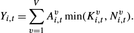
We denote with ![]() the purchase of a machine tool of vintage v. The firm will choose the vintage on the basis of the ratio of the expected future productivity of each vintage for a firm relative to the price of the machine tool of that vintage
the purchase of a machine tool of vintage v. The firm will choose the vintage on the basis of the ratio of the expected future productivity of each vintage for a firm relative to the price of the machine tool of that vintage ![]() . When calculating the estimated future productivity of a vintage,
. When calculating the estimated future productivity of a vintage, ![]() , the firm takes into account that the skills of its workforce will evolve over time and that this evolution is influenced by the vintage the workers are matched with. The probability of selecting a given vintage is then determined by means of the multinomial logit model:
, the firm takes into account that the skills of its workforce will evolve over time and that this evolution is influenced by the vintage the workers are matched with. The probability of selecting a given vintage is then determined by means of the multinomial logit model:
(54)
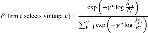
where ![]() . In EUBI the K-firm sets the price
. In EUBI the K-firm sets the price ![]() using a weighted average between a cost- and value-based pricing component. To determine the value-based component, the firm estimates the expected future productivity of each vintage for a firm with a labor force whose skill profile matches the average profile in the economy.
using a weighted average between a cost- and value-based pricing component. To determine the value-based component, the firm estimates the expected future productivity of each vintage for a firm with a labor force whose skill profile matches the average profile in the economy.
MABMs considered so far rule out substitutability among inputs (they assume indeed perfect complementarity). An exception to this rule is EUGE. The setting is similar to EUBI: there is complementarity between the quality of the capital stock and the skill composition of the labor force. The actual productivity of firm i is determined by the average quality of its capital stock, ![]() , and the average skill of the workforce,
, and the average skill of the workforce, ![]() . EUGE, however, assume that technology to produce output is represented by a Cobb–Douglas production function:
. EUGE, however, assume that technology to produce output is represented by a Cobb–Douglas production function:
(55)
Hence inputs are substitutable. While technology in EUBI is characterized by complementarity (i) of skill and vintage and (ii) of labor and capital, in EUGE there is complementarity of skill and quality of capital, but substitutability of labor and capital.
2.4.3 Demand and Supply of Capital Goods
In the market for K-goods (K-market, for short), C-firms are buyers and K-firms are sellers.
Decisions of C-firms concerning capital accumulation have long term effects on the production possibilities of the firm. A few approaches have been proposed to describe and interpret investment decisions in a complex environment in which firms cannot perfectly anticipate future developments on goods and factor markets.
In LAGOM firms enter the market for K-goods with demand ![]() where
where ![]() is the production target of the firm.
is the production target of the firm.
In CATS/ADG, in each period the firm decides on capacity utilization and on investment. The two decisions are carried out independently. By assumption, the firm copes with short run oscillations of demand by adjusting capacity utilization (if feasible). Investment, on the contrary, is driven by long run production requirements, as we shall see momentarily.
Let's assume that, on the basis of expected demand, the firm plans in period t to produce ![]() in period
in period ![]() . In period
. In period ![]() , the capital stock will be
, the capital stock will be ![]() where
where ![]() is the depreciation rate,
is the depreciation rate, ![]() is the utilization rate, and
is the utilization rate, and ![]() is investment decided in period t. There are two scenarios.
is investment decided in period t. There are two scenarios.
If the capital stock is “large”, i.e., ![]() , the firm will reach the desired scale of activity by setting capacity utilization at the required level
, the firm will reach the desired scale of activity by setting capacity utilization at the required level ![]() with
with ![]() .
.
If, on the contrary, the capital stock is “insufficient”, i.e., ![]() , the firm will use machinery and equipment at full capacity but will produce less than desired because its scale of activity is constrained by the available capital stock
, the firm will use machinery and equipment at full capacity but will produce less than desired because its scale of activity is constrained by the available capital stock ![]() .
.
Investment decisions in period t are based on the stock of capital the firm has used on average until period ![]() , computed by means of the following adaptive rule:
, computed by means of the following adaptive rule: ![]() where
where ![]() . By iterating, it is easy to see that
. By iterating, it is easy to see that ![]() is a weighted average of past utilized capital with exponentially decaying weights:
is a weighted average of past utilized capital with exponentially decaying weights:
(56)

The history of capacity utilization in the past, therefore, will influence the decision to purchase new capital goods in period t and this decision, in turn, will impact on capacity in the future.
The firm is assumed to have a target long run capacity utilization rate ![]() . Therefore the capital desired at the investing stage t for
. Therefore the capital desired at the investing stage t for ![]() is
is ![]() . Investment to replace worn out capital is
. Investment to replace worn out capital is ![]() . Hence total investment will be
. Hence total investment will be ![]() where
where ![]() .
.
CATS/ADG assume, moreover, that there are adjustment costs of the capital stock such that only a fraction of C-firms is capable to purchase new capital goods in each period. Hence the firm has to take into account the fact that investment can be carried out only infrequently. Durability and stickiness imply that the capital stock available for production at the beginning of period ![]() keeps memory of the entire history of the capital stock in the past.
keeps memory of the entire history of the capital stock in the past.
The demand side of the market for K-goods if populated by C-firms. The ith C-firm plans to purchase K-goods in the amount ![]() .
.
Consider now the supply side, which is populated by ![]() K-firms. Each K-firm has market power due to transaction costs (e.g., incompleteness of the information set) which force C-firms to visit only a subset of the population of K-firms. The ith C-firm, in fact, does not interact globally with all the producers of machine tools but randomly selects
K-firms. Each K-firm has market power due to transaction costs (e.g., incompleteness of the information set) which force C-firms to visit only a subset of the population of K-firms. The ith C-firm, in fact, does not interact globally with all the producers of machine tools but randomly selects ![]() K-firms, sorts them by selling price and demand capital goods starting from the firm charging the lowest price. K-firms with lower prices, therefore, will get, in principle, higher demand.
K-firms, sorts them by selling price and demand capital goods starting from the firm charging the lowest price. K-firms with lower prices, therefore, will get, in principle, higher demand.
At the beginning of time t the kth producer of capital goods (![]() ) sets the status quo
) sets the status quo ![]() .
.
Once production has been carried out65 and search and matching has taken place, the kth firm observes the amount of K-goods actually sold ![]() where
where ![]() is actual demand, coming from C-firms which placed orders at firm k.
is actual demand, coming from C-firms which placed orders at firm k.
If production is greater than demand, the firm will pile up an involuntary inventory of unsold goods. Since K-goods are storable, inventories accumulated in period t can be used to satisfy demand in the future. If, on the contrary, demand is greater than production, the firm can satisfy excess demand by depleting inventories carried oven from the past.
K-firms receive two signals like C-firms: the price charged by competitors and the change of inventories or the presence of queues. On the basis of these signals, the firm changes the price or the quantity. Price and quantity updating rules for K-firms are similar to those adopted by C-firms, the major difference being the assumption that machine tools can be stored in warehouses in period t and sold to C-firms in the future.
In EUBI the ith C-firm purchases new machine tools if the current capital stock is not sufficient to produce planned output. EUBI define potential output as production the firm can carry out in period t using at full capacity the capital stock inherited from the past in the absence of investment, i.e., ![]() . The investment decision is the outcome of a comparison between potential output and desired output
. The investment decision is the outcome of a comparison between potential output and desired output ![]() .
.
If the capital stock inherited from the past is “large”, ![]() , the firm can produce desired output by adjusting capacity utilization and there is no investment. If desired production is greater than potential output, so that the capital stock inherited from the past is “insufficient”, the firm expands the capital stock and investment is positive. The size of the investment depends on the vintage v chosen by the firm for the investment in that period (see (54)):
, the firm can produce desired output by adjusting capacity utilization and there is no investment. If desired production is greater than potential output, so that the capital stock inherited from the past is “insufficient”, the firm expands the capital stock and investment is positive. The size of the investment depends on the vintage v chosen by the firm for the investment in that period (see (54)):
(57)
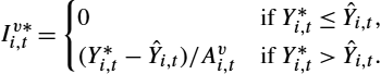
Due to the flexibility in production due to input substitutability, in EUGE the capital-to-labor ratio is a function of the relative costs of the inputs:
(58)
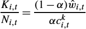
where ![]() is the real wage and
is the real wage and ![]() is the user cost of capital, a function of the real interest rate, the depreciation rate, and the price of K-goods.
is the user cost of capital, a function of the real interest rate, the depreciation rate, and the price of K-goods.
Plugging (58) into (55) and rearranging, we get the demand for capital as
(59)
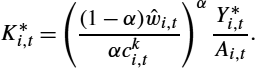
If the current capital stock in the absence of investment is smaller than desired capital, the firm adjusts capacity utilization. If the opposite holds true, the firm purchases new capital goods to bring capital up to the desired size.
K-firms produce and sell tailor-made machine tools to each purchasing C-firm, using only energy and raw materials, imported from abroad. The price of machine tools is a mark-up on energy prices. Since they follow a job production process, K-firms don't have inventories. By construction, moreover, they don't have financing needs.
In KS, as in CATS/ADG, for simplicity, K-firms produce machine tools of different vintages using only labor. K-firms send “brochures” to selected C-firms advertising the price and the quality of the machine tools they produce. C-firms compare brochures and then choose the machines with the lowest price and unit cost of production and send their orders to the corresponding machine manufacturer. Gross investment of each C-firm is the sum of expansion and replacement investment, where, as above, expansion happens if the desired level of production is higher than what can be produced with the current capital stock.
2.4.4 The Demand for Labor
In LEN, AGH, and JAMEL, quantity decisions translate immediately into hiring/firing decisions. In LEN, thanks to the one-to-one technology, vacancies are derived straightforwardly from the quantity adjusting rule. If inventories are “too low”, the firm will post a new vacancy to increase production. In symbols, ![]() if
if ![]() . If, on the contrary, inventories are “too high”, the firm will fire a worker in order to reduce production,
. If, on the contrary, inventories are “too high”, the firm will fire a worker in order to reduce production, ![]() if
if ![]() .
.
The firm adjusts the posted wage according to the following rule:
(60)

where ![]() is drawn from a uniform distribution.
is drawn from a uniform distribution.
In JAMEL maximum employment per firm coincides with the capital stock. Hence we can define capacity utilization ![]() . JAMEL assume also that there is a target or desired utilization rate
. JAMEL assume also that there is a target or desired utilization rate ![]() . The firm adjusts the posted wage according to the following rule:
. The firm adjusts the posted wage according to the following rule:
(61)
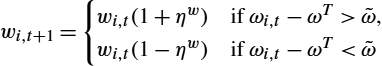
where ![]() is drawn from a uniform distribution and
is drawn from a uniform distribution and ![]() is a stochastic cut-off value.
is a stochastic cut-off value.
In AGH the firm conducts market research before deciding to enter the market and produce by sending out messages to people who are prospective employees. This message contains the posted wage. AGH assume that the wage is set by the firm as
(62)
where ![]() is a function of the ratio of desired employment to the workforce,
is a function of the ratio of desired employment to the workforce, ![]() , and
, and ![]() is expected inflation, which is equal to the (time invariant) inflation target of the central bank. AGH assume that the central bank's target for inflation is the anchor agents used in expectation formation.
is expected inflation, which is equal to the (time invariant) inflation target of the central bank. AGH assume that the central bank's target for inflation is the anchor agents used in expectation formation.
In most MABMs with capital, the demand for labor is determined by planned production and the size of the capital stock, with limited substitutability between labor and capital. Consider, for instance, CATS/ADG. Let's assume that, on the basis of expected demand, the C-firm plans to produce ![]() in period
in period ![]() . Suppose that technology is represented by a Leontief production function (see above). If the capital stock is “large”, then
. Suppose that technology is represented by a Leontief production function (see above). If the capital stock is “large”, then ![]() . Hence the firm could reach the desired scale of activity by setting capacity utilization at the required level and adjust desired employment accordingly. In symbols,
. Hence the firm could reach the desired scale of activity by setting capacity utilization at the required level and adjust desired employment accordingly. In symbols, ![]() .
.
If, on the contrary, the capital stock is “insufficient”, the firm will use the stock of capital at full capacity (![]() ) and
) and ![]() so that desired employment in this case will be
so that desired employment in this case will be ![]() . Hence planned employment will be
. Hence planned employment will be
(63)
where ![]() and
and ![]() .
.
In EUBI and EUGE, if the capital stock is “too low” in a given period, say, ![]() , investment can be carried out in the same period to overcome bottlenecks in production, also in the short run (see previous section) so that
, investment can be carried out in the same period to overcome bottlenecks in production, also in the short run (see previous section) so that ![]() .
.
In EUBI, with a Leontief technology, the demand for labor is
(64)
The same equation defines the demand for labor in LAGOM.
In EUGE, with a Cobb–Douglas technology, the demand for labor is
(65)
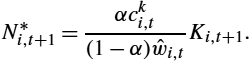
Given planned employment ![]() and actual employment,
and actual employment, ![]() , at the beginning of period
, at the beginning of period ![]() the firm posts vacancies as follows:
the firm posts vacancies as follows:
(66)
Suppose ![]() . In CATS/ADG, a vacancy is filled only if the firm is visited by an unemployed worker. The probability of filling the vacancy depends on the posted wage and on the number of unemployed workers visiting the firm. Thus actual employment
. In CATS/ADG, a vacancy is filled only if the firm is visited by an unemployed worker. The probability of filling the vacancy depends on the posted wage and on the number of unemployed workers visiting the firm. Thus actual employment ![]() may be smaller than desired employment
may be smaller than desired employment ![]() , the difference between the two being unfilled vacancies. In this case the planned scale of activity will not be reached.
, the difference between the two being unfilled vacancies. In this case the planned scale of activity will not be reached.
Suppose now ![]() , i.e., the number of actual workers exceeds the level of desired employment. In this scenario the firm fires
, i.e., the number of actual workers exceeds the level of desired employment. In this scenario the firm fires ![]() workers selected at random. Similarly, in EUBI the actual workforce can differ from planned employment due to search frictions and differences in wages offered by different firms If employment is too high, there is random firing.
workers selected at random. Similarly, in EUBI the actual workforce can differ from planned employment due to search frictions and differences in wages offered by different firms If employment is too high, there is random firing.
Summing up, the firm enjoys full flexibility in adjusting production when production must be scaled down (first scenario) and when output should be increased but “not too much” (i.e., when capacity utilization can be adjusted adequately). When the desired increase in output is sizable the firm hits a capacity constraint.
Actual production may be smaller than desired if the firm does not succeed in achieving the “appropriate” level of capital but also if the firm does not succeed in achieving the “appropriate” level of employment (for instance because of unfilled vacancies) and/or she does not get enough credit.
Consider now K-firms. In CATS/ADG, the kth firm produces output ![]() by means of a linear technology which uses only labor,
by means of a linear technology which uses only labor, ![]() where α is the productivity of labor, exogenous, constant, and uniform across firms. Desired employment will be
where α is the productivity of labor, exogenous, constant, and uniform across firms. Desired employment will be ![]() . The firm posts vacancies
. The firm posts vacancies ![]() . These vacancies add to those posted by C-firms.
. These vacancies add to those posted by C-firms.
On the labor market C-firms and K-firms are competing for labor services: labor is a homogeneous input. Unemployed workers search for a job visiting ![]() firms (out of a population of F firms) irrespective of the type of goods they produce. In other words, the unemployed worker is indifferent between finding a job at a C-firm or a K-firm.
firms (out of a population of F firms) irrespective of the type of goods they produce. In other words, the unemployed worker is indifferent between finding a job at a C-firm or a K-firm.
2.4.5 The Demand for Credit
In most MABMs, the demand for credit comes from the corporate sector only and is determined by the firms' financing needs. Consider a generic firm, say, f (where ![]() ), with operating costs
), with operating costs ![]() and internal funds
and internal funds ![]() . If the latter is greater than the former, the firm can finance costs by means of internal funds only. If, on the contrary, costs are greater than internal funds, the firm has a financing gap
. If the latter is greater than the former, the firm can finance costs by means of internal funds only. If, on the contrary, costs are greater than internal funds, the firm has a financing gap
(67)
which must be filled by means of a bank loan. The demand for credit, therefore, coincides with the financing gap.66
Consider a C-firm. If technology requires only labor, operating costs coincide with the wage bill. Hence the financing gap is ![]() . This is essentially the demand for credit in AGH, LEN, and JAMEL.67
. This is essentially the demand for credit in AGH, LEN, and JAMEL.67
If the firm employs labor and capital, the firm has to finance also the purchase of new K-goods. For example, in CATS/ADG the expenditure on capital goods is ![]() where
where ![]() represents the price index of K-goods.68
represents the price index of K-goods.68
Consider now a K-firm. If technology requires only labor, the financing gap is ![]() .
.
We can posit, therefore, the following general specification of the demand for credit:
(68)
where ![]() is an indicator function which assumes value 1 if the firm employs capital and labor and 0 if it employs only labor.
is an indicator function which assumes value 1 if the firm employs capital and labor and 0 if it employs only labor.
2.5 The Bank
In most MABMs, C-firms demand labor and K-goods in order to produce and sell C-goods to households.
2.5.1 Credit Risk and the Interest Rate
The Benchmark: Financial Frictions
In the most recent literature, a special and crucial role for financial factors in macroeconomic performance stems from the assumption of “financial frictions”, i.e., imperfections in the transmission of funds from surplus units (lenders) to deficit units (borrowers).69 There are essentially three types of financial friction.
Costly State Verification
Building on Bernanke and Gertler (1989, 1990), Bernanke et al. (1999) (BGG hereafter) develop an NK-DSGE model, in which a financial friction arises from ex post asymmetric information between borrowers (“entrepreneurs”70) and lenders (banks) in the presence of costly state verification á la Townsend. Information on the return of investment becomes asymmetric ex post, i.e., after the investment has been carried out. While the entrepreneur can observe the return on investment at zero cost, the bank can ascertain the “true return” only incurring a monitoring cost.
To be more specific, consider the balance sheet of the representative entrepreneur
(69)
where K is physical capital (a durable asset), q is the market value of the firm's assets, L is debt towards banks, and E is net worth. Hence ![]() is leverage.71 The optimal financial contract between the entrepreneur and the bank in such a setting yields a risk premium, i.e., a wedge between the interest rate on loans and the risk free interest rate, which BGG label the “External Finance Premium” (EFP),
is leverage.71 The optimal financial contract between the entrepreneur and the bank in such a setting yields a risk premium, i.e., a wedge between the interest rate on loans and the risk free interest rate, which BGG label the “External Finance Premium” (EFP), ![]() .72 They show that the EFP is increasing with the borrower's leverage,
.72 They show that the EFP is increasing with the borrower's leverage, ![]() with
with ![]() . In the end, therefore
. In the end, therefore
(70)
In BGG the bank sets (optimally) the interest rate on loans (i.e., the price of credit) as a mark-up over the risk free interest rate, the mark-up being increasing with leverage. At that price all the credit demanded is extended. The quantity of credit is demand-driven.
Costly Enforcement
Kiyotaki and Moore (1997) (KM hereafter) assume that the human capital of the producer/borrower is critical to production and “inalienable” á la Hart and Moore. In this setting there is financial friction due to costly enforcement of the debt contract: if the borrower “takes the money and runs”, the lender cannot replace him with a new producer as producers are not substitutable. In a default scenario the lender is bound to experience a loss. Therefore she will design the debt contract in such a way as to minimize this loss.
The debt contract specifies the interest rate (![]() ), the size of the loan (L), maturity (one period), and the provision of collateral (K) on the part of the borrower. Due to costly enforcement, the borrower is subject to a financing constraint
), the size of the loan (L), maturity (one period), and the provision of collateral (K) on the part of the borrower. Due to costly enforcement, the borrower is subject to a financing constraint
(71)
where ![]() is the loan the lender is willing to extend,
is the loan the lender is willing to extend, ![]() is a durable asset pledged by the borrower as collateral, which we will identify with “capital”,73
is a durable asset pledged by the borrower as collateral, which we will identify with “capital”,73 ![]() is the price of capital at maturity,
is the price of capital at maturity, ![]() is the interest rate on loans, uniform across agents, given and constant. The financing constraint states that the lender extends a loan in period t of a size such that debt commitments (interest and principal)
is the interest rate on loans, uniform across agents, given and constant. The financing constraint states that the lender extends a loan in period t of a size such that debt commitments (interest and principal) ![]() at maturity, i.e., at time
at maturity, i.e., at time ![]() , is equal to the market value of collateral
, is equal to the market value of collateral ![]() . Thanks to the financing constraint, if the borrower defaults, at maturity the lender can repossess capital and sell it, earning sales proceeds
. Thanks to the financing constraint, if the borrower defaults, at maturity the lender can repossess capital and sell it, earning sales proceeds ![]() exactly equal to the borrower's debt commitments. The lender's loss in case of default therefore is reduced to zero.
exactly equal to the borrower's debt commitments. The lender's loss in case of default therefore is reduced to zero.
Plugging (71) into (69) and rearranging, we get ![]() where
where ![]() is leverage.74 Hence, leverage is increasing with
is leverage.74 Hence, leverage is increasing with ![]() but decreasing with
but decreasing with ![]() and
and ![]() .
.
In KM the quantity of credit is set by the lender as a proportion of the market value of collateral. The price of credit is exogenous.
If the production function is ![]() , then the scale of activity of the producer will be constrained by his wealth (net worth):
, then the scale of activity of the producer will be constrained by his wealth (net worth):
(72)
Costly Bankruptcy
Greenwald and Stiglitz (1993) (GS hereafter) shift the burden of bankruptcy costs from the lender to the borrower. For GS it is the borrower who incurs the (pecuniary and reputational) costs due to default. These costs are the source of financial friction, which shows up as a wedge between the interest rate on loans as perceived by the borrower and the cost of credit set by the lender.
Consider a generic firm which gets a loan ![]() from a bank at the rate R. Debt commitments therefore are
from a bank at the rate R. Debt commitments therefore are ![]() . The firm incurs bankruptcy costs
. The firm incurs bankruptcy costs ![]() with probability
with probability ![]() . GS assume that the costs of bankruptcy are increasing with size:
. GS assume that the costs of bankruptcy are increasing with size: ![]() where
where ![]() is the (given) cost of default per unit produced. Moreover, they show that when revenues are uncertain, the probability of default is increasing with leverage,
is the (given) cost of default per unit produced. Moreover, they show that when revenues are uncertain, the probability of default is increasing with leverage, ![]() ,
, ![]() . Hence total costs (the sum of debt commitments and expected bankruptcy costs) are
. Hence total costs (the sum of debt commitments and expected bankruptcy costs) are ![]() where
where ![]() is output per unit of credit. The actual cost of credit (i.e., the interest rate on loans for the borrower) therefore is
is output per unit of credit. The actual cost of credit (i.e., the interest rate on loans for the borrower) therefore is
(73)
The actual cost of credit is the interest rate set by the bank augmented by a risk premium ![]() borne by the borrower. It is the borrower who perceives the risk of default. In Bernanke et al. (1999), the risk of default is borne by the lender.75
borne by the borrower. It is the borrower who perceives the risk of default. In Bernanke et al. (1999), the risk of default is borne by the lender.75
The Agent-Based Approach to Interest Rate Setting
In AGH, there is a bank in each sector of the economy, loosely defined as a subset of the number of goods. The bank accepts deposits from people in its sector and extend loans to firm owners. Loans are collateralized by inventories and fixed capital (which plays only the role of collateral, it is not an input). If a firm is unable to reimburse debt the bank can repossess all the collateral and the wealth of the firm owner (money and deposits) (“full recourse”). The interest rate on deposits is equal to the interest rate set by the central bank. In many ABMs the interest rate set by the central bank is either fixed or follows a Taylor rule. For instance, in AGH, LAGOM, KS, and EUGE, the interest rate is assumed to follow a standard Taylor rule in the flexible inflation targeting regime
(74)
where ![]() is the target for the “long run” interest rate76 and
is the target for the “long run” interest rate76 and ![]() are the targets for inflation and output, respectively. While
are the targets for inflation and output, respectively. While ![]() is fixed, in AGH the target for potential output and the target for the long run interest rate are updated. The interest rate on loans is a fixed markup on this rate, uniform across firms.
is fixed, in AGH the target for potential output and the target for the long run interest rate are updated. The interest rate on loans is a fixed markup on this rate, uniform across firms.
In CATS/ADG firms demand credit according to their production plans and the resulting financing gaps (as shown above). For simplicity, there is only one bank, which has to decide both the price (interest rate) and the quantity of loans to extend to each firm on the basis of the assessment of the firm's financial fragility proxied by leverage.
For each borrowing firm f in each period the bank can compute the leverage ratio ![]() .77
.77
The bank will estimate the relationship between the individual bankruptcy probability ![]() and the individual leverage
and the individual leverage ![]() as
as ![]() . The estimated default probability is an increasing function of leverage.
. The estimated default probability is an increasing function of leverage.
For simplicity, the bank is assumed to be risk neutral: it will lend to a risky firm inasmuch as the return on lending to that firm is not smaller than the return on investing in an alternative risk free asset which measures the opportunity cost of lending.78
Once all the arbitrage opportunities have been exploited, the following equality will hold true: ![]() . Hence
. Hence
(75)
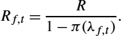
From (75) it follows that the interest rate charged by the bank to the fth firm is increasing with the risk free rate and with the firm's leverage. This is a reduced for a BGG type of friction. If the firm goes bankrupt, the equity of the bank will decrease.
Also in JAMEL there is only one bank, which accommodates the demand for credit at a fixed interest rate r and maturity ![]() (uniform across borrowing firms). If a firm, say, firm i, enters a period of financial distress and becomes unable to validate debt commitments as scheduled, the loan becomes “doubtful” so that the bank raises the interest rate to
(uniform across borrowing firms). If a firm, say, firm i, enters a period of financial distress and becomes unable to validate debt commitments as scheduled, the loan becomes “doubtful” so that the bank raises the interest rate to ![]() and extends maturity to
and extends maturity to ![]() .
.
In EUBI and EUGE, the bank assesses the probability of default as follows:
(76)
The interest rate charged by the bank to the firm therefore is given by
(77)
where k is a parameter.
2.5.2 Supply of Loans
In most MABMs, the bank is subject to a regulatory prudential constraint consisting of a minimum “capital requirement” of the Basel type: the bank must have “capital” (net worth) ![]() at least equal to a given fraction of risky assets
at least equal to a given fraction of risky assets ![]() . Defining the bank's leverage as
. Defining the bank's leverage as ![]() , the regulatory constraint can be recast in terms of maximum leverage: the bank can hold illiquid (risky) assets up to a maximum equal to a multiple
, the regulatory constraint can be recast in terms of maximum leverage: the bank can hold illiquid (risky) assets up to a maximum equal to a multiple ![]() of net worth. In symbols,
of net worth. In symbols, ![]() where
where ![]() is the bank's upper bound on bank's leverage set by the regulator.
is the bank's upper bound on bank's leverage set by the regulator.
In AGH, risky assets are ![]() where
where ![]() is the level of seized collateral. The probability for the bank to approve new loan applications is
is the level of seized collateral. The probability for the bank to approve new loan applications is
(78)
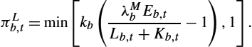
The bank will extend loans for sure if ![]() , i.e., if
, i.e., if ![]() . When this threshold is achieved, the probability of approving a new loan becomes less than one. It becomes zero when the maximum regulatory requirement is reached, i.e.,
. When this threshold is achieved, the probability of approving a new loan becomes less than one. It becomes zero when the maximum regulatory requirement is reached, i.e., ![]() .
.
In CATS/ADG and KS, risky assets coincide with loans. Hence the regulatory constraint boils down to ![]() . Suppose the constraint is binding. Hence the maximum amount of credit the bank can extend to all firms/borrowers is constrained by the availability of internal finance:
. Suppose the constraint is binding. Hence the maximum amount of credit the bank can extend to all firms/borrowers is constrained by the availability of internal finance:
(79)
At this point the bank has to allocate credit to each firm. CATS/ADG assume that bank b opens a credit line ![]() to firm f up to a maximum represented by a fraction
to firm f up to a maximum represented by a fraction ![]() of total credit
of total credit ![]() . This fraction is decreasing with the firm's leverage:
. This fraction is decreasing with the firm's leverage: ![]() with
with ![]() . In symbols,
. In symbols, ![]() . KS posit a similar procedure: borrowing firms are ordered in terms of financial fragility, captured by the ratio of net worth to past sales.
. KS posit a similar procedure: borrowing firms are ordered in terms of financial fragility, captured by the ratio of net worth to past sales.
If the loan demanded by the firm (i.e., the financing gap ![]() ) is smaller than the maximum loan the bank is willing to extend (i.e.,
) is smaller than the maximum loan the bank is willing to extend (i.e., ![]() ), then the bank will accommodate the demand for credit,
), then the bank will accommodate the demand for credit, ![]() ; if, on the contrary, the financing gap is greater than the credit line the bank is willing to extend, the bank will limit credit to the borrower,
; if, on the contrary, the financing gap is greater than the credit line the bank is willing to extend, the bank will limit credit to the borrower, ![]() . In the end therefore,
. In the end therefore,
(80)
From the inequality above, given the definition of a financing gap, it follows that an increase of the net worth of the bank and/or of the borrowing firm – so that the firm's leverage and the estimated probability of bankruptcy go down – relaxes the constraint represented by the maximum admissible loan supply and makes credit rationing less likely.
In EUBI and EUGE, the bank computes the budget available to fund firms as follows:
(81)
where ![]() is the sum of risk weighted assets in the bank's portfolio. The bank has to decide now how much credit to extend to each firm. In EUBI, the firm's financing gap is funded completely if the credit risk exposure remains below the budget, while the firm is fully rationed if the loan exceeds this limit.
is the sum of risk weighted assets in the bank's portfolio. The bank has to decide now how much credit to extend to each firm. In EUBI, the firm's financing gap is funded completely if the credit risk exposure remains below the budget, while the firm is fully rationed if the loan exceeds this limit.
3 Comparison of Existing Agent-Based Macroeconomic Models
Whereas in the previous section we have discussed in some detail several key issues in designing MABMs, the purpose of this section is to provide a more general survey and comparison over several agent-based macroeconomic models, which have been developed during these years. We discuss the variance of the model structure and the behavioral assumptions across the different approaches and examine in how far an established “core” of modeling assumptions has emerged for agent-based macroeconomics. The basis for this discussion are Tables A1 and A2 in Appendix A, which provide a systematic overview of main properties of the eight agent-based macroeconomic models that have already been the basis for the discussion in Section 2.
The different models covered here have been designed and implemented for various research purposes in macroeconomics and with different agendas in mind.
- • MABMs, in which “financial factors” play a major role in business fluctuations: AGH, CATS, EUGE;
- • MABMs, in which capital accumulation, embodied technical progress, and skill dynamics generate growth, fluctuations, and inequality dynamics: KS, EUBI;
- • MABMs with focus on policy analyses, in particular on certain measures in fiscal, monetary or climate policy: KS, EUBI, EUGE, LAGOM;
- • MABMs, which capture the effects of learning of agents, social influence, and opinion dynamics: JAMEL;
- • MABMs with minimal complexity that are able to reproduce key stylized facts like endogenous business cycles, Phillips and Beveridge curves: LEN.
The presentation of the models in Tables A1 and A2, as well as our discussion of the similarities and differences between the different models, is structured along eight broad categories covering different aspects of the setup of the models and their main output. As observed in Section 2, in terms of the general model structures, we observe that almost all share the same set of types of agents (households, C-firms, K-firms, banks, policy makers) and considered markets (consumption goods, capital, labor, credit, stocks) except for LEN, which does not include physical capital, credit, and banks in the model, and AGH, which also abstracts from physical capital accumulation. Recent literature on agent-based macroeconomics has stressed the importance of the concept of stock-flow consistency for models of this type (e.g., Caiani et al., 2016a). Stock-flow consistency entails that the model is closed in a sense that for any transaction the (real and financial) flows of all involved agents sum up to zero, such that there are no (hidden) inflows or outflows. This can be most easily ensured if the model encompasses explicit balance sheets for all agents, but only a fraction of the MABMs have these properties, and therefore it is not straightforward to verify this property if it is not directly reported by the authors.
In terms of other general properties, it becomes clear that in most MABMs expectations are mainly considered with respect to the future development of firm demand, whereas expectation formation of households about future income or economic developments is often not considered. The employed expectation rules are in most MABMs naive or linear forecasts. An exception in this respect is JAMEL, which models the dynamics of household expectations driven by evolving sentiments in the population. In term of agent demographics, the considered MABMs do not incorporate an evolving age structure of individuals and keep the number of agents of different types constant over time. Firm entry occurs in most models only after a firm has exited the market and thereby is essentially a replacement of the exiting firm (with different firm characteristics and equity). Only the AGH model captures, in a rather sophisticated way, the market entry of firms and the associated decisions of potential entrants as well as financial transactions. A simple endogenous firm entry process, in which the (stochastic) number of entrants in a sector depends positively on the number of incumbents in the industry, as well as on the sectoral ratio between firms' liquid assets and debt, has also been incorporated in a recent version of the KS model (see Dosi et al., 2017b). Although the possibility to consider spatial structures and (emerging) heterogeneities of distributions of agents characteristics across regions arguably is a merit of the agent-based modeling approach most of the models so far have not considered multiregional settings. Exceptions in this respect are EUBI and LAGOM, which have been used for numerous analyses of economies with multiple regions or countries. Recently, also multicountry versions of the KS (Dosi et al., 2017d) and the EUGE model (Petrovic et al., 2017) have been put forward and Caiani et al. (2017) have developed a stock-flow consistent multicountry model to analyze different fiscal regimes in a currency union.
Considering the consumption goods market, the focus of the different models, in particular whether they aim to explain endogenously economic growth and technological change, shows clearly in the way the production process is covered. Whereas KS and EUBI incorporate vintage structured capital goods and endogenous vintage choices of firms, the other MABMs consider capital with homogeneous productivity,79 which is typically combined in fixed proportion with labor to produce the consumption good. As discussed in the previous section, assuming mark-up pricing is most common, where the mark-up is typically adjusted over time based on the firms' market share or its inventory level (relative to expected demand). Only EUBI features a different approach in which firms explicitly estimate the form of the demand function they are facing. Quantity choices in most models are determined by the expected demand (typically adjusted by a security buffer and the current stock of inventory), in JAMEL and LEN the output quantity is determined by the size of the labor force, which, however, is adjusted over time based on the relationship between expected demand and inventory.
The size of the physical investment of consumption good firms is in most models simply derived from the potential need of expansion due to the current production plan. In these investment rules long run planning has no effect on the investment patterns, which is arguable rather myopic, since the acquired physical capital will be available for the firm for an extended period of time. An exception in this respect is CATS, where investment is based on a target level of capital, which is calculated from past capital requirement over an extended time interval. Whereas this rule seems less myopic, it still does not involve any explicitly forward looking planning of the firm. Harting (2015) has developed an extension of the EUBI model, in which investment is determined in a forward looking way using a real-option approach. Also, in most MABMs the firm's demand for inputs (capital and labor) are dictated by the decision on the scale of activity, which is typically driven by observed past demand for the goods produced by the firm. Potential changes in the price of the different inputs do not play any allocative role. For instance, the demand for capital (labor) by a C-firm is determined by the expected sales of the firm, which in turn is determined by the (past) consumer's demand. Changes in the price of capital (labor) hence do not enter the considerations determining the current demand for these inputs. Exceptions in this respect are EUBI, where the estimated unit costs of production, which are determined by input prices, influence price, and quantity decisions, and EUGE, where, although input prices do not influence the planned production level, they determine the desired capital-to-labor ratio.
With respect to the determination of the households' consumption budget, (piecewise) linear rules based on the wealth and income have emerged as the dominant choice in the design of MABMs. In particular, a large fraction of model relies on buffer stock rules put forward in Carroll and Summers (1991), which also have strong empirical and theoretical foundations. Also the matching between households and consumption good producers is modeled in similar ways across the considered models, in which explicit protocols for this matching procedure are given. Consumers observe the prices of a randomly selected subset of consumption good producers and then select (with high probability) the cheapest ones. If they cannot purchase the full amount they demand, households move to the next best option, and so on. A different approach in this respect is chosen in AGH, where customers have evolving networks of stores to which they have relations and then buy from these firms in a way to maximize their utility.
The capital good markets in the considered MABMs typically have a much simpler structure than the consumption goods markets, since it is usually assumed that there is no explicit quantity choice of producers who simply produce based on orders they have received. Also, apart from the KS and the CATS model, no competition between capital good producers is considered. With respect to pricing there is a large heterogeneity of the considered pricing rules including fixed mark-up rules, prices based on anticipated value of the capital good for consumption good producers and pricing rules based on expected demand and inventory similar to approaches used for the consumption good market. In the EUBI and the KS model, endogenously evolving sets of multiple vintages of capital goods are considered. Whereas in the EUBI model new vintages emerge randomly, the KS model incorporates an explicit representation of the innovation activities in the capital goods sector such that the probability of a firm to innovate depends on its R&D investments.
Also with respect to the interactions on the labor market there is considerable uniformity across the MABMs. Labor demand is derived from the planned output, and with the exception of Dosi et al. (2017b, 2017c) none of the considered models explicitly captures inertia in the adjustment of the stock of workers that might, for example, be driven by labor market regulations or labor contract durations.80 The majority of MABMs relies on random search of job-seekers in combination with posted wages of firms having vacancies, where posted wages are adjusted if the searching firms are unable to fill their vacancies. In several MABMs (EUBI, EUGE, KS, LAGOM) wages are also adjusted according to the evolution of labor productivity. In EUBI and EUGE the productivity of a worker is strongly influenced by her skills, which evolve endogenously over time. No such skill differentiation is present in the other (standard) models although a recent version of the KS model also exhibits heterogeneous and endogenously evolving skills of workers (Dosi et al., 2017b). Furthermore, dynamically adjusting reservation wages, which rely mainly on the worker's current (wage or unemployment) income, determine in several of the models, whether workers accept the jobs with the posted wages.
External financing of firms is in all considered models, with the exception of EUGE, restricted to bank loans. With respect to the interest rate the banks charge to firms, the majority of MABMs follows an approach where a mark-up, whose size depends on the borrowers leverage and riskiness, is applied to the Central Bank interest rate. On the other hand, there is substantial heterogeneity across the models with respect to possible rationing of firms on the credit market. Whereas in some MABMs all credit demands are satisfied (JAMEL, LAGOM), others introduce probabilities of loan approvals (AGH, CATS) or assume (regulatory) upper bounds on the volume of credit a bank can grant (EUBI, EUGE, KS). A common feature of the credit market in combination with the investment rules in the considered models is that firms do not take into account the induced interest payments when deciding on their output and investment targets, although the amount of credit they need influences their financial standing and thereby their interest rate and size of interest payments. Hence, the impact of the central bank base rate and of the shape of the interest rule the banks use typically is weak in these models. With exception of the Eurace models, none of the MABMs includes a stock market. Also in EUBI only a minimalistic stock market is considered in which an index share, containing all firms in the economy, is traded. EUGE incorporates a more complex stock market in which different shares are traded.
Only a subset of the considered models assigns an active role to the government, and also in these models government activity essentially reduces to collecting income and profit taxes in order to be able to pay out unemployment benefits and potentially implement additional fiscal policy measures, like paying out firm subsidies. In all these models, tax rates are dynamically adjusted over time to fulfill a balanced budget or a target debt to GDP ratio. Different variations of the Taylor rule are the dominant choice to determine the central bank interest rate; however, in several of the MABMs the interest rule is also treated as fixed model parameter.
This brief discussion highlights that in spite of the heterogeneity with respect to the agenda and objective of the different MABMs a consensus has emerged in the MABM community about a number of key features of behavioral rules and interaction protocols. A similar statement can certainly be made about empirical validation of the models. The reproduction of stylized facts has become a standard way to show that the developed MABMs are able to capture important economic mechanisms that are responsible for business cycle properties and distributional characteristics in real economies. As Tables A1 and A2 clearly show, many of the MABMs have been very successful in qualitatively matching stylized facts on different levels of aggregation, combining the reproduction of average levels of key variables with time series properties and distributional patterns. Clearly, this point is one of the perceived main strengths of the agent-based approach in (macro)economics, although it has to be observed that clear quantifiable standards for what is exactly meant by the “reproduction” of a stylized fact is so far missing. The last few years have seen a significant increase in the work trying to quantify the quality of the match between simulation output generated by agent-based models and empirical data (e.g., Guerini and Moneta, 2017; Barde, 2017), as well as approaches for systematic estimation of agent-based models in Economics (e.g., Grazzini et al., 2017). This work is discussed in more detail in the chapter by Lux and Zwinkels (2018) in this handbook, and we refrain from a detailed treatment here.
4 Policy Analysis
Early work in agent-based macroeconomics, as well as in agent-based studies of individual markets, was mainly concerned with showing that agent-based models are able to capture important empirical features of real world economic dynamics and with exploring implications of different assumptions about individual behavior and interaction schemes. The last ten years, however, have seen a considerable increase in agent-based work with a policy focus. Several reasons might have contributed to this development. First, the financial and economic crisis unfolding after 2008 highlighted the need of building policy analyses on models capable of capturing mechanisms, which are potentially responsible for the outbreak of crises, as well as describing economic dynamics far away from an equilibrium state. In particular, the interplay between real and financial markets, contagion effects, dynamic expectation formation, and similar issues came to the forefront of attention for policy makers, and clearly agent-based models are well suited to deal with these issues. Second, the work in agent-based macroeconomics has seen some consolidation in the sense that a number of models (many of them have been discussed in the previous sections) have been systematically developed and improved over a considerable time span. Improved confidence in the ability of these models to capture key economic mechanisms, e.g., by building on their ability to reproduce a wide range of stylized facts, has also made them a more reliable basis for policy analysis. Some of these models have been developed into something like “workhorse” models for policy analysis and have been used for the exploration of the effects of policies in a diverse range of domains. Third, the accumulating evidence in Experimental and Behavioral Economics that individual behavior is often not determined by (intertemporal) optimization and rational expectations has generated increasing attention in macroeconomics for studying learning and adaptive expectation formation and for investigating policy effects in models capturing these phenomena. Several of the agent-based contribution to the policy literature are addressing this point.
Apart from these developments, several other well-known properties of the agent-based approach models seem particularly useful in the context of policy analyses. This includes the ability to distinguish explicitly between short-, medium-, and long-run effects of policies, as well as to capture potential path dependencies and hysteresis effects triggered by policies. Furthermore, the fact that agent-based models are designed to represent the evolution and emergence of heterogeneities of different kinds makes them well suited to generate insights about the implications of different policies for the distribution of key economic indicators and therefore also for studying inequality in the economy.
In the following subsections we briefly review agent-based policy analysis in different key policy domains. We have decided to organize the discussion of existing policy studies in this way although several of the covered papers combine the analysis of different types of policy measures, as well as their interaction, in a unified framework. Hence, several papers will appear in more than one of the following subsections. Having discussed several contributions in different policy areas, we will conclude this section with some general comments about how agent-based policy analyses have developed over the last decade.
It should be stressed that we restrict our coverage to contributions which analyze policy effects in the framework of macroeconomic models. For several of the policy domains covered there is also a very active agent-based literature relying on partial models, e.g., addressing issues of systemic risk. Furthermore, also in some areas outside the domains, which are covered in the following sections, policy related work using an agent-based approach has been done. This includes in particular the area of environmental and climate policy, where some recent contributions develop integrated assessment models linking the approaches developed in agent-based macroeconomics with some climate module capturing dynamics and effects of climate change. These models seem to have high potential for the analysis of different types of climate-relevant policies. A survey over this emerging literature can be found in Balint et al. (2017).
4.1 Fiscal Policy
An early analysis of fiscal policy effects in the framework of an agent-based macromodel is carried out in Russo et al. (2007). The main agenda of this paper is to compare the effect of demand oriented versus technology oriented fiscal measures in the presence of endogenous technological change. A simple macroeconomic model containing only goods and labor markets is considered with random matching protocols on both markets (incorporating loyalty effects on the labor market) and simple adaptive behavioral rules governing price and wage adjustment. Production technology is linear with labor as the single input and the firm-specific labor productivity stochastically evolves over time where the expected increase depends on the firm's R&D investment. Since it is assumed that firms invest a fixed fraction of their profits in R&D, the model exhibits a positive relationship between firm sales and the speed of technological change.
After the discussion of emergent properties of the model and of several empirical stylized facts it is able to reproduce, Russo et al. (2007) focus on a computational experiment aimed at exploring the qualitative consequences of alternative fiscal policies. In particular, they consider two scenarios in which a public agency introduces a (flat) tax rate on firms' profits. In the first scenario these tax revenues are paid out as unemployment benefits, whereas in the second scenario they are redistributed to firms on a per-capita basis increasing their R&D expenditures. The simulations show a strongly diverging effect of the tax on the average growth rate in these two scenarios. In the first scenario, in which the tax is used to boost demand, the effect on growth is clearly negative and becoming stronger the higher the tax rate. In the technology oriented scenario, a positive effect on growth is detected, which grows with the tax rate as long as the rate stays below an upper threshold. These results show that in the considered setting the multiplier generated by higher demand is not sufficiently large to outweigh the direct negative effects of the tax on R&D spending, which hinges on after-tax profits. The main driver of the positive effect of a technology oriented redistributive tax policy seems to be the intensification of R&D activities per se rather than the redistribution between firms. This is demonstrated by comparing the effect of an increase in tax rate with a scenario without the tax in which firms increase their R&D rates by the same amount. It is shown that the growth rate in the second scenario, referred to as private R&D scenario, is always above that in a corresponding public R&D scenario, in which R&D is entirely financed through the tax. This suggests that the tax per se has a negative effect on economic performance. The question whether it is needed to induce the desirable level of R&D expenditures cannot be addressed in the considered setting since the R&D rate is a given exogenous parameter rather than an endogenous result of firms' decision making.
Whereas in Russo et al. (2007) the positive effects of fiscal policy measures are rather limited, most of the following agent-based fiscal policy analyses come to much more positive conclusions about the effectiveness of fiscal measures, both with respect to fostering growth and to reducing business cycle fluctuations. Haber (2008) uses the agent-based macroeconomic model “AS1”, incorporating geographical structure, evolving product ranges, a rather sophisticated banking sector, and explicit expectation formation processes, to analyze the effect of an expansionary fiscal policy on key economic indicators. In particular, the implications of a reduction of the tax rate on income and firm profits is studied. It is shown that such a reduction leads to an increase in economic growth, as well as a reduction in unemployment and increase in inflation. Using the fact that the model can capture a variety of different expectation formation rules, Haber (2008) also demonstrates that the positive effect of the fiscal expansion is reduced if the agents employ more sophisticated foresight mechanisms. In any case, the reduction of the tax rate induces a higher level of public debt, which in the framework of the model is covered through bank credit.
The potential growth enhancing effect of an expansionary fiscal policy has also been an important theme in the analysis of fiscal measures in the framework of the “Keynes meeting Schumpeter” (KS) model. In Dosi et al. (2010) the effects of a rise in the level of unemployment benefits financed by an increase of the tax rate on firm profits is studied. It is shown that increasing the rate of unemployment subsidies relative to wages (and therefore also the tax rate) from zero to a positive level has a significant positive effect on the growth rate of productivity and output, where the actual size of the positive rate has only little influence. The authors explain this observation in a way that in the absence of unemployment subsidies the low demand negatively affects firms' R&D investment and thereby also negatively affects productivity growth leading to a vicious cycle associated with low growth and strong fluctuations. A minimal level of fiscal stimulation is needed to avoid such a low growth scenario and to allow the economy to fully exploit the technological opportunities for productivity growth arising in the considered framework. Whereas the level of a positive unemployment and tax rate hardly affects the speed of growth, increasing these rates leads to reduced output volatility and reduced unemployment. This analysis is extended in Dosi et al. (2013), where it is shown that the positive effects of such a fiscal policy, which redistributes firm profits to households, is larger the more market power the firms have. More precisely, the authors establish that the reduction in volatility and unemployment induced by higher unemployment subsidies and tax rates is more pronounced if firms charge a high price mark-up on consumption goods. If mark-ups are so low that the economy is persistently in (almost) full employment an increase in the unemployment subsidy/tax rate yields an increase of growth rate volatility. These observations reinforce that in the framework of this model the main role of the considered fiscal measures is to channel funds from firm savings to households, where it stimulates demand. The authors stress that their results highlight the importance of the interactions between income distribution regimes and redistributive fiscal policies.
The observation in Dosi et al. (2010, 2013) that fiscal measures can reduce economic fluctuations illustrates a theme that has been an important motivation of numerous agent-based studies of fiscal policy, namely that this type of policy models are well suited to examine the mechanisms by which fiscal policies might trigger or avoid crises and to explore potential fiscal policy responses to crises once they have emerged. In Dosi et al. (2015) the dynamics of the KS model in the benchmark case with constant unemployment subsidy/tax rate is compared to scenarios in which these rates are adjusted according to rules resembling the European Stability and Growth Pact (SGP) and the European Fiscal Compact (FC). In particular, under these rules the level of unemployment subsidies is reduced if the deficit is above 3% of GDP, in case of SGP, or, in case of FC, public expenditures have to be cut also if public debt exceeds the target of 60% of GDP. For both types of rule also an adjusted version with escape clause is considered, in which these constraints do not apply in periods in which the growth rate is negative. The simulation results clearly indicate that compared to the benchmark both rules without escape clauses have significant and large negative effects on growth and employment. Furthermore, they strongly increase output volatility and the likelihood of economic crises. Due to these negative implications for the level of economic activity in the framework of this model, the considered rules even induce exploding dynamics of public debt to GDP ratios. In the presence of escape clauses the negative implications of these fiscal rules are much weaker, however, with the exception of the effects on the growth rate, still significant. The authors conclude from these observations that an unconstrained fiscal policy allowing automatic stabilizers is needed to dampen economic fluctuations and to reduce the likelihood of crises. They also discuss the interplay of such a policy with different variants of monetary policies (see Section 4.2).
The results of Dosi et al. (2015) that fiscal contraction in bad times yields negative implications for recovery and growth is consistent with evidence presented in the framework of other agent-based macroeconomic models. A study closely related to that of Dosi et al. (2015) is carried out by Teglio et al. (2018) in the framework of the Eurace simulator (EUGE). They also consider the effects of fiscal rules, corresponding in a stylized way to the European Stability and Growth Pact (SGP) and the European Fiscal Compact (FC), and combine them with an escape clause and a “fiscal accommodation” (reduction of tax rates during crises), as well as with quantitative easing by the central bank. Similar to Dosi et al. (2015) they find that applying escape clauses and fiscal accommodation both to the SGP and the FC reduces the probability of depressions and increases average growth rates. Napoletano et al. (2015) study in the framework of a simple endowment economy with a credit market the effectiveness of different fiscal policies in the aftermath of a (household) bankruptcy shock. They show that a deficit-spending rule is able to reduce the negative impact of the bankruptcy shock on the economy and to favor a fast recovery from the recession more effectively than balanced-budget policies. Furthermore, the size of the fiscal multiplier is time-varying and is largest in the downturn several periods after the shock. Neveu (2013) uses a model, which in structure is similar to that of Russo et al. (2007), however, with a slightly different fiscal setup. Fiscal revenues are generated by a combination of a corporate profit tax and a progressive income tax and are spent partly on unemployment benefits and partly on R&D subsidies for firms, which are distributed across firms proportionally to last period profits. Three fiscal rules are considered, in which special measures are activated once the economy contracts for four successive periods: (i) fiscal spending is increased while the tax rate is kept constant; (ii) spending and taxes are cut such that a balanced budget is maintained; (iii) the tax rate is reduced while spending is kept constant. Under the first and the third rule, public debt is accumulated during downturns, and during growth periods taxes are adjusted to repay this debt. It turns out that all three rules have no significant effect on average growth or unemployment, however, differently from rules (i) and (ii) the third rule reduces the number of long downturns significantly and substantially. Hence, a debt financed stimulation of demand and R&D during bad times helps to avoid long and deep recessions without negatively affecting growth perspectives even if the debt accumulated during downturns is repaid during growth periods.
Similarly to Neveu (2013), also Harting (2015) studies the implications of different fiscal responses to downturns on the growth rate and volatility of the economy. In the framework of an extended version of the Eurace@Unibi model (EUBI), the following three scenarios are compared, where in each a special fiscal policy is activated once the growth rate of output drops below a given threshold. In the first scenario households receive a direct fiscal transfer, thereby increasing their consumption budget, in the second scenario all firms receive subsidies on any investment they make, whereas in the third scenario subsidies are paid out only to firms investing in the best available vintage of the capital good. Since in the Eurace@Unibi model the vintage choice of firms is determined by the comparison of the ratio of expected future return to price of each vintage, the third rule influences the technology choice of firms and fosters the acquisition of frontier vintages. Main insights from the analysis in Harting (2015) are that all three policies are able to reduce the volatility in the economic dynamics. However, in order to achieve the same reduction of volatility, the demand oriented first measure requires substantially larger fiscal expenditures during the downturns than the other two technology oriented rules. Furthermore, the three rules differ substantially with respect to their growth effects. No such effects are induced by the second measure, i.e., the payout of subsidies to all investing firms. The other two rules have positive growth effects and these effects are much stronger if the third rule is used, in which only firm investment in frontier technology is subsidized. These results imply that the facilitation of diffusion of new technologies in the economy is the main driver of the positive effects of these policies.
While the papers reviewed in the previous paragraphs have focused on the role of fiscal policy measure as automatic stabilizers and as instruments to prevent crises and economic fluctuations, Dawid et al. (2018c) examine which types of fiscal measures are most effective in fostering recovery and growth in a region which is in an economic crisis. The agenda of the paper is motivated by the developments associated with the public debt crises in southern European countries unfolding after 2010. This paper uses a two-region version of the Eurace@Unibi (EUBI) model and considers a scenario where the two regions are in an economic union with integrated consumption and capital goods markets but differ substantially with respect to size as well as the technological level of firms and the (specific) skill endowment of workers. In particular, a scenario is considered in which the smaller and technologically lagging region has accumulated so much public debt that it no longer has access to the credit market. Without any fiscal transfers from the larger and faster growing region this situation would lead to a rigorous decline in output and consumption in the small region. The paper compares the effects of different union-wide financed fiscal transfer schemes to the crisis region and shows that technology oriented subsidy policies, which are able to positively influence the technology choice of firms in the lagging region is the only option to foster long-run catch-up of the that region. The effect of this policy becomes significant only after a considerable delay, whereas measures strengthening demand in the lagging region have a positive short-run effect on consumption in that region, however, with little positive impact on production and productivity. A policy in which only the debt burden of the lagging region is taken over by the union has no significant positive effect on the economic dynamics in that region. The paper shows that under none of the considered policy measures the larger and stronger region in the union, which covers the majority of the fiscal expenditures, experiences significant negative effects on consumption or production.
4.2 Monetary Policy
A strong focus of agent-based work with a policy orientation has also been on monetary policy issues and the optimal design of regulatory schemes for banks and the financial market. We will survey contributions concentrating on regulatory issues in the next subsection and concentrate here on studies of classical monetary policy instruments, in particular interest rate rules.
Dosi et al. (2013) study the implications of a variation of the (constant) central bank interest rate in the framework of the KS model. In their setting a variation of the interest rate in the range between 0% and 10% essentially has no impact on the level or on the fluctuations of growth rates. Only as the rate is increased beyond this level to some value, which depends on the firms' market power, a strong negative impact on the growth rate associated with increasing fluctuations emerges. For sufficiently high levels of firm mark-up such negative impact of interest rate increases is, however, avoided. The intuition underlying these results is that the interest rate negatively affects growth performance mainly by increasing the danger of firm bankruptcies, which destabilize the economy, and by reducing the frequency of full employment states. Under sufficiently high mark-ups the risk of bankruptcies is negligible and hardly affected by the interest rate. Hence the effect of interest rate hikes are very minor.
While Dosi et al. (2013) assume a fixed central bank interest rate, the majority of contributions rely on variations of the Taylor rule to model the central bank's interest rate policy. Raberto et al. (2008) demonstrate that a simple output gap oriented interest rule, at least if it is sufficiently strong, leads to better economic performance in terms of output and worker utility compared to a random interest rule. In a related work, Delli Gatti and Desiderio (2015) compare the performance of an economy under a fixed central bank rate and an output and inflation oriented Taylor rule in the aftermath of a negative productivity shock. They show that with a Taylor rule the decrease in output is much weaker and the price level stays lower compared to the fixed interest scenario. The main positive effect of the Taylor rule in this setting is that it helps to keep the firms' credit demand and liquidity higher than under a fixed central bank rate. Ashraf et al. (2016) consider in the framework of the AGH model a Taylor rule based on inflation and output gap and study the implications of a variation of the central bank's (fixed) inflation target on output, inflation, and volatility. Quite in accordance with the insights in Dosi et al. (2013), they find that increasing the inflation target above a certain threshold leads to a deterioration of output and an increase in volatility. The interpretation of Ashraf et al. (2016) for these results is that a large inflation target induces a large dispersion of relative prices increasing the frictions on the goods market and thereby the bankruptcy risk of sellers.
Several agent-based studies have explored how changes in the set of target variables as well as in the values of the reaction coefficients in the Taylor rule affect the emerging economic dynamics and also how these effects depend on various properties of the considered economy. Dosi et al. (2015) compare the economic dynamics emerging in the KS model if the central bank targets only inflation with that under a Taylor rule with dual mandate reacting to inflation and unemployment. They find that the dual mandate rule significantly increases the growth rate in the economy and that the positive growth effect is particularly strong if a restrictive fiscal policy is in place. This growth effect also is associated with a reduction in unemployment. Furthermore, the dual mandate leads to less GDP volatility compared to a purely inflation oriented monetary policy. The authors explain the positive effect of the dual mandate rule by a better performance of the banking sector, reducing the rate of bank failures and increases the number of investment projects that are financed and implemented.
Contributions by Krug (2015) and Chiarella and Di Guilmi (2017) use different agent-based macroeconomic models to examine in how far a Taylor rule, which takes into account some indicator of economic instability, can improve economic performance and stability. Krug (2015) develops an agent-based macromodel, which combines a simple real sector with exogenous growth with a quite detailed representation of the money market and the financial sector. He examines the implications of an extension of a dual mandate Taylor rule (inflation and output gap), which either reacts also to the deviation of a financial stability indicator from its target value or reacts also to the deviation of the credit to GDP ratio from its long term trend. A main finding of the paper is that also with such an extension of the policy rule, monetary policy alone cannot achieve significant improvements with respect to financial stability if the goal of macroeconomic stability remains the main focus. Combining a dual mandate Taylor rule with macroprudential policy in form of a more rigid regulation of the financial sector seems much more efficient in this respect. The paper highlights also that implementing a “leaning against the wind” monetary policy (i.e., a Taylor rule reacting with a central bank rate increase to an increase of the financial instability indicator) in a restrictive regulatory environment is counterproductive and actually leads to higher financial fragility. Chiarella and Di Guilmi (2017) also study the effects of a policy oriented towards financial stability by considering a Taylor rule which includes the deviation of the current fraction of Ponzi firms from its past moving average as a financial instability indicator. Motivated by the seminal work of Minsky (1963), firms are classified as Ponzi if they have positive debt and negative profit. Quite in accordance to the main insights from Krug (2015), they also find that increasing the (positive) reaction coefficient of the central bank rate to the fraction of Ponzi firms leads to a larger rather than a smaller fraction of Ponzi firms in the economy and does not reduce the bankruptcy rate. Furthermore, such a change in the monetary policy has a negative impact on aggregate output.
While the work discussed in the previous paragraph has highlighted the suitability of an agent-based approach to study the interplay of monetary policy and regulation, works by Salle et al. (2013) and Salle (2015) exploit the ability of this approach to capture heterogeneous expectation formation processes and learning in a macroeconomic framework. They consider a macroeconomic model with social learning among households and individual learning of firms in which the central bank uses a nonlinear Taylor rule responding to inflation and unemployment. Salle et al. (2013) examine the impact of an increase of the reaction coefficients of inflation and unemployment under different credibility scenarios for the central bank. They find that monetary policy is much more effective if the central bank's target rate can be communicated with full credibility and is perceived without noise. In Salle et al. (2013) the inflation expectations of households are formed in a very simple way as a weighted average between the perceived inflation target and the past inflation. In Salle (2015) a much more sophisticated and flexible expectation formation process is inserted into this macroeconomic model. This process is modeled using artificial neural network with different sets of input variables which vary according to the considered transparency scenario. These input variables might also include the central banks internal inflation forecasts, based on VAR models, or the trend of these forecasts. The analysis of extensive simulation exercises under the different scenarios shows that transparency of the central bank reduces the trade-off between the goals of inflation targeting and minimization of the output gap. In particular, it turns out that a central bank which communicates not only its objectives but also its forecasts reduces the inflation-output gap trade-off and should use smaller reaction coefficients to these two objectives than a central bank restricting communication to its objectives.
In addition to the extensive work studying the impact of different interest rate rules of the central bank on economic performance, agent-based models have also been used to explore the macroeconomic effect of quantitative easing. Cincotti et al. (2010) use the Eurace simulator (EUGE) to compare quantitative easing scenarios, in which the central bank purchases government bonds, thereby financing public deficits, with fiscal tightening. Under fiscal tightening the deficit of the government is funded by issuing new bonds in the market and by an increase of tax rates. The effects of the two policies are compared under different assumptions about the dividend payout ratio of firms, where higher dividend ratios imply a larger demand of firms for external credit and therefore a higher amount of credit in the economy. The authors show that quantitative easing leads to higher growth rates in the economy and to higher inflation compared to the fiscal tightening scenario. The effect is much stronger in scenarios with a relatively small dividend payout rate. Also Chiarella and Di Guilmi (2017) combine their analysis of variations of the Taylor rule, which was discussed above, with policy experiments based on a central bank rule determining the supply of money. In particular, the supply of central bank money is assumed to depend negatively on inflation and on the number of Ponzi firms in the economy. In the exogenous money scenario, in which only the central bank, but not the financial sector, can generate money, an increase of each parameter capturing the effect of inflation and Ponzi firms on money supply reduces the number of Ponzi firms. In the endogenous money scenario, in which the financial sector endogenously generates all credit demanded by firms and liquidity demanded by investors, increasing the sensitivity parameter with respect to inflation also reduces the variance of output fluctuations.
4.3 Financial Regulation and Crisis Resolution Mechanisms
On of the main policy lessons learned from the financial and economic crisis of 2007 is that systemic risk matters and should be taken into account when designing regulatory policies. This has not only led to the development of the Basel III framework for the regulation of the financial sector, but also to an explosion of academic work studying the implications of different regulatory schemes from a systemic perspective, which acknowledges the interconnectedness of the players in the financial sector, as well as the feedbacks between the real and the financial sector. An agent-based approach seems a natural choice to transform such a perspective into concrete models and indeed a number of contributions based on such an approach have improved our understanding of the macroeconomic effects of different regulatory instruments discussed in the aftermath of the crisis.
Teglio et al. (2012) use the Eurace simulator (EUGE) to analyze the effect of making the regulatory capital requirement, defined in terms of the ratio of equity to risk-weighted assets, more restrictive. They find that a very strong requirement, which implies some credit rationing of firms from the start of the simulation, has negative implications for short-term GDP in the economy, however, induces higher output and lower unemployment in the long-run compared to a looser regulatory scheme. They argue that under a more restrictive scheme the buildup of financial fragility of firms is avoided, which leads to more significant credit rationing of firms in the long-run under loose regulatory schemes. In Cincotti et al. (2012b) this analysis is extended by considering capital requirements which are adapted over time in a countercyclical way, i.e., they become more tight in good times compared to bad times. Two versions of such rules are considered, where the level of unemployment and the amount of total credit are used as indicators of the state of the economy. Simulations indicate that in the long run output is higher and unemployment is lower under such adaptive policies compared to fixed capital requirements. This effect is particularly strong if the countercyclical policy is based on total credit in the economy. Raberto et al. (2018) explore in the framework of the Eurace simulator (EUGE) how a capital adequacy requirement for banks, which requires lower reserves for firm loans compared to household mortgages, might foster firms investment in new technologies and the transition to green energy production. They find that such regulatory schemes in the short-run indeed speed up firm investment in new technologies, but at the same time reduce overall growth due to stronger constraints on household expenditures. In the long-run this negative effect outweighs the positive one even with respect to firm investment.
van der Hoog and Dawid (2018) pose the question which type of banking regulation is best suited to avoid large downturns in an economy. Within the framework of the Eurace@Unibi model (EUBI) they use indicators developed in the empirical literature to identify amplitude and duration of recessions and expansions in the simulation data and analyze how the distribution of these indicators depends on the regulatory environment. In particular, they compare the effects of strengthening the capital requirement with those of making the reserve requirement, which focuses on a bank's liquidity, more stringent. They find that if the capital requirement becomes more restrictive, the distribution of recession amplitudes shifts in a way that the amplitudes of the most severe recession become larger and overall strong recessions become more likely. If the reserve requirement becomes more restrictive, an opposite effect is observed and the distribution of amplitudes becomes more concentrated around smaller values. Based on their examination of the mechanisms underlying these observations, which involves the categorization of firms according to their financial status, the authors argue that a liquidity constraint is able to prevent banks from fueling a debt bubble that is mainly caused by the financially unsound firms requiring new debt to roll-over old debt. Hence, strict liquidity requirements reduce the risk of large downturns. In a related work van der Hoog (2018) shows, again in the framework of the Eurace@Unibi (EUBI) model, that a stringent reserve requirement reduces the output fluctuations without negatively affecting the (average) dynamics of total output.
An extensive agent-based analysis of the effect of different types of regulatory schemes for banks is also carried out in Popoyan et al. (2017). They build their analysis on an extension of the AGH model, in which the banks' rule for granting loans to shops is based on a frequently used approach for determining creditworthiness, the “6C” approach. The main objectives of the study are to compare the economic dynamics under a Basel II type regulation of banks with that under a Basel III approach, and to analyze which aspects of the Basel III regulation are most crucial for the effectiveness of that scheme. In particular, the paper distinguishes between the following four regulatory instruments, which are all part of the Basel III scheme: (i) a static capital requirement; (ii) a countercyclical buffer, as an add-on to the capital requirement, which is determined based on the aggregate private sector credit-to-GDP ratio; (iii) a leverage requirement; (iv) a liquidity requirement. Considering the level and the volatility of output gap and unemployment, as well as the likelihood of crises, the authors find that the Basel III scheme performs significantly better than Basel II. More specifically, the combination of the static capital requirement with the countercyclical buffer seems to be the crucial aspect of the Basel III approach. Implementing just these two instruments already yields results that are only slightly worse than those under the full Basel III package. However, applying only the leverage requirement or only the liquidity requirement produces significantly larger output gaps and unemployment values, as well as more volatility. The authors show that in their setting these instruments alone perform worse than the Basel II rule. These claims are verified across different Taylor rules that are inserted into the model. Comparing these findings with those of van der Hoog and Dawid (2018) and van der Hoog (2018) discussed above, one has to acknowledge that, whereas the importance of the countercyclical buffer seems consistent with the intuition of the importance of bubble prevention in these papers, the negative role of the liquidity constraint is at odds with the main findings in van der Hoog and Dawid (2018) and van der Hoog (2018). This observation highlights the importance of taking into account the details of the underlying macroeconomic setup when interpreting the qualitative insights from policy analyses. Riccetti et al. (2018) employ still another agent-based macroeconomic framework and show that, similar to the finding reported above, also in their setting a too loose capital-based banking regulation increases financial fragility with potential negative implications for the real economy. However, they also point out that an overly tight regulation, which restricts the availability of credit too strongly, is detrimental for the performance of the economy.
The papers we have discussed in this section so far have focused on the regulation of regular commercial banks. Krug and Wohltmann (2016) point out that in recent years actors other than commercial banks, which are not subject to the corresponding regulation, have taken over a more important role of financial intermediaries in the economy. They analyze the impact of such shadow banks on the dynamics and stability of the economy in a stock-flow-consistent agent-based macroeconomic model, in which banks are subject to Basel III type regulation. Inserting unregulated shadow banks into a benchmark scenario, in which only commercial banks offer financial services, the authors find a destabilizing effect of the informal financial sector on the economy. At the same time they find a small positive impact of the informal financial sector on the growth rate. If the shadow banks are also subject to regulation and share the traditional banks' access to central bank liquidity, then the variance of output, as well as that of inflation, is, however, substantially lower than in the benchmark. Based on this, the authors argue that including the shadow banks in the regulation and giving them access to the central bank as lender of last resort is helpful for reaching the central bank's dual mandate of price and output stabilization. At the same time the average growth rate of output is substantially smaller in such a scenario with regulated shadow banks compared to the benchmark.
The regulatory environment of the financial sector is not only determined by the constraints banks face while solvent, but also by the mechanisms that apply in case a bank is defaulting. Klimek et al. (2015) compare the macroeconomic effect of three different types of such crisis resolution mechanisms in the framework of a simple agent-based macroeconomic model. These mechanisms are: (i) a purchase and assumption (P&A) operation under which assets and liabilities of the defaulting bank are taken by the other banks; (ii) a bail-out under which households and firms provide equity for the bank; (iii) a bail-in under which unsecured claims of creditors are written off or transformed to equity. In all cases the mechanism is activated if the equity of a bank falls below a certain (negative) threshold. The effect of these different mechanisms on output, unemployment, and credit volume is compared for different levels of the banks refinancing interest rate (which drives the size of the interest rate the bank is charging the firms). For low interest rates, the choice of the crisis resolution mechanism has little effect, but for higher interest rates bail-in and bail-out lead to better results than P&A. In particular, in the highest interest rate regime, which is characterized by high unemployment and low household savings the bail-in mechanism leads to highest output and lowest unemployment because in such a setting the financial burden for firms and households, implied by the bail-out of banks, significantly affects their level of economic activity reducing the overall output in the economy.
4.4 Labor Market Policy
The discussion in the previous subsection highlights that, in particular after the crisis of 2008, the focus of the (agent-based) literature dealing with market regulation has been on the financial and credit market. However, in the framework of agent-based macroeconomic models also the effects of regulatory schemes on other markets, in particular the labor market has been studied. An example in this respect is Seppecher (2012), who in the framework of the JAMEL model, shows that higher flexibility of (reservation) wages decreases unemployment duration, but through the demand channel reduces consumption and real wages and increases unemployment.81 The introduction of a minimum wage in such a scenario can help to eliminate such negative effects of increased wage flexibility.
The findings of Seppecher (2012) are consistent with results obtained in the framework of other agent-based studies, like Napoletano et al. (2012) and Dosi et al. (2017c). In the latter paper the authors compare the effects of different labor market regimes in the framework of a version of the KS model with a decentralized labor market. A “Fordist” regime, in which wages are indexed to productivity, firms do not dismiss workers as long as profits are positive and workers do not search on the job, is compared to different variations of a “Competitive” regime, in which wage changes respond to unemployment, firms immediately adjust the size of their work force to their current production plan and workers search for a job. The main insight from their analysis is that in scenarios, where growth is mainly driven by demand, the Competitive regime's no full indexation of minimum wages and no unemployment benefits are associated with higher unemployment, slower growth, and a higher risk of economic crises compared to the Fordist regime. The main mechanism underlying this observation is that, under the Competitive regime without wage indexation, wages and thereby demand are strongly diminished during downturns, which reduces firm investment in R&D and new vintages, which reduces the rate of productivity growth. In a similar setting and following a similar logic, Dosi et al. (2018) show that the Fordist regime also induces lower unemployment and lower income inequality than alternative regimes under which firms have higher flexibility in dismissing workers. In Dosi et al. (2017b) the Fordist and Competitive labor market regimes are compared with respect to the question how much hysteresis an economy exhibits under these regimes. The model of Dosi et al. (2017c) is extended by incorporating endogenous skill dynamics of workers into the model and also introducing endogenous firm entry and the main focus of the analysis is on the question how strong and how long lasting the negative impact of a crisis on future growth is. Quite consistent with the results of the two papers just discussed, the authors find that under a Fordist regime the negative impact of a crisis is substantially less severe and also shorter-lived than under a competitive regime.
In Dawid et al. (2018b) the effect of increasing the flexibility of the labor market is studied in a two-region version of the EUBI model in which the two regions differ with respect to (initial) firm productivity and worker skills (see also Section 4.5). In particular, it is studied how the growth and inequality in the weaker region is affected if the wage replacement rates in that region are decreased and the pressure to find work are increased such that the workers' reservation wages adjust downwards much faster if they are unemployed. Whereas such measures induce a decrease of the growth rate of output in that region, they also reduce the income inequality in the region. Both effects arise because under a more flexible labor market technologically less advanced firms in the region have better chances to hire workers who have been earning higher wages at firms with higher productivity before. This reduces the wage dispersion in the population and at the same time increases competition for the high productivity firms reducing their investment and thereby reducing overall productivity growth.
4.5 Regional Growth, Convergence, and Cohesion Policy
In a stream of papers different versions of the Eurace@Unibi model (EUBI) have been used to study how different types of (region-specific) policies influence the regional dynamics of growth and technological change in an economy consisting of several heterogeneous regions. In Dawid et al. (2008) a two-region version of the model is considered and it is assumed that a certain budget is available to improve the general skills, i.e., the speed by which workers can acquire specific skills that increase their productivity. The main question posed is how the effects of an equal distribution of the skill upgrading measures across the two regions compare to an approach where all effort is concentrated in one region (“lighthouse policy”). It is shown that the equal distribution leads to higher average productivity and output in the economy in the long-run, whereas a concentration of effort induces faster growth in the short-run. A crucial assumption for this finding is that labor is immobile across regions. This implies that firms in the lighthouse region, which due to their productivity advantages in the short-run also have cost and price advantages relative to firms from the other region, face problems filling their vacancies with local workers once the demand for their products becomes too large. These rationing problems on the labor market inhibit output expansion and growth and also induce upwards pressure on wages in the lighthouse region. If the upgrading of skills is equally distributed across the regions such effects do not occur, which explains why such an equal distribution yields better outcomes in terms of economy-wide output and productivity growth.
The importance of spatial labor market frictions for the results in Dawid et al. (2008) is highlighted in Dawid et al. (2009), where the same policy experiment is carried out under a completely integrated labor market of the two regions (no commuting costs for workers working in the other region from where they live) and a market with positive, but small commuting costs. Not surprisingly, in the case of a completely integrated labor market the allocation of the skill upgrading measures between regions is irrelevant, however, for small positive commuting costs the opposite result to Dawid et al. (2008) is obtained. Concentrating all skill upgrading measures in one region here leads to higher economy-wide output in the long-run. The impact of different degrees of labor market integration on regional economic dynamics and economy wide output is studied in more detail in Dawid et al. (2012). Again, a two-region version of the Eurace@Unibi (EUBI) is studied, in which the first region (the “high-tech” region) is characterized by a larger fraction of workers with high general skills and an initial advantage of the local firms with respect to the quality of their physical capital stock compared to the second region (“low-tech”). Inspired by discussions about the integration of labor markets between EU member countries after the EU enlargement in 2004, the authors compare the economic dynamics emerging under four different policies: (i) full separation of labor markets; (ii) full integration (no commuting costs); (iii) integration with small commuting costs between regions; (iv) integration with small commuting costs with some delay (after the integration of the product markets). A main finding of this paper is that, whereas in terms of economy-wide long-run output open labor markets clearly outperform closed ones, the ranking of the different policies differs crucially depending on which region and which time horizon is considered. For the high-tech region closed labor markets are preferable in terms of the level of produced output if the planning horizon is short, while under a long-run consideration open labor market with small frictions perform best. For the low-tech region the opposite holds true. Closed labor markets are harmful in the short-run but have positive long run implications for this region. The underlying mechanisms are again closely related to the induced labor flows across regions, the resulting pressure on wages, and the associated investment incentives of firms.
A demonstration how multiregion agent-based macromodels can be used to provide insights into the effects and the effectiveness of cohesion policies aiming at the fostering of convergence between regions is given in Dawid et al. (2014, 2018b). In particular, these papers incorporate policy measures resembling instruments the European Union applies as part of its cohesion policy in a two-region setting of the Eurace@Unibi (EUBI) model, in which, similar to Dawid et al. (2012), one region has an initial advantage with respect to physical and human capital endowment. In Dawid et al. (2014) the effects of two types of cohesion policies are analyzed, namely a human capital oriented policy, under which the distribution of general skills in the low-tech region is improved, and a technology oriented policy, under which firms in the low-tech region receive subsidies if they invest in new physical capital at the technological frontier. It is shown that in a scenario with integrated labor markets between the two regions the human capital policy fails to achieve its objective of fostering convergence between the two regions, but, quite on the contrary, affects only the output in the high-tech region positively. The output in the low tech region, which is the target of the policy, is, however, negatively influenced. The reason for this observation is that the human capital policy induces a flow of highly skilled workers from the low tech region to firms in the high tech region, which due to their higher productivity offer higher wages. This has second order effects on firms' investment incentives, which give rise to this result. If labor markets are separated, then the human capital policy indeed facilitates growth in the low-tech region and therefore fosters convergence. Considering the effect of the technology policy, it is shown that it always fosters convergence, and that the effect is stronger if labor markets are integrated. Dawid et al. (2018b) focuses entirely on the effects of technology policies and shows that the positive convergence effect identified in Dawid et al. (2014) disappears if the policy becomes “undirected” in a sense that investing firms in the low-tech region receive subsidies even if they invest off the technological frontier. In this paper the effect of cohesion policies is not only studied with respect to the income differences between the two regions but also with respect to income inequality within each region.
4.6 Taking Stock: What Is the Potential of Agent-Based Macroeconomics for Policy Analysis?
Several general observations about the use of agent-based models for policy analysis can be made based on the literature review in this section. There seems to be a clear development both with respect to content and to methodological standards. Whereas the earlier contributions reviewed above, let's say most of the papers from 2008 to 2013, have mostly focused on rather generic and traditional policy issues, like interest rate policies or demand versus supply oriented fiscal polices, many of the more recent publications explore the implications of rather detailed aspects of actual policy proposals. These contributions exploit the ability of the agent-based approach to capture institutional details of environments and policies to disentangle the implications of different aspects of programs like the Basel III regulations or the EU cohesion policies. Clearly, such insights about the expected effects of details in the policy design should be highly relevant for policy makers. Similarly, the consideration of the interplay of different types of policy measures, as well as the feedback between policies, expectations, and credibility of policy makers, which has been the focus of several of the reviewed contributions, seems to be an important aspect of the agent-based work in the policy domain.
From a methodological perspective, a trend towards statistical rigor in the analysis of policy effects can be observed over the last decade. The (often graphical) comparison of the means across Monte Carlo runs of certain considered variables between different policy scenarios, which has been quite common in earlier contributions, has more or less disappeared in more recent publications. Providing meaningful statistical tests for the significance of certain policy effects, or at least confidence bands around for the considered variables under the different policy variants has become a standard in the literature. Also, more sophisticated methods have been applied, like the use penalized spline methods for the estimation (also providing confidence bands) of the dynamics of the isolated effects of certain policies in simulation models (Dawid et al., 2014, 2018b, 2018c; Harting, 2015) or regression analyses of the impact of policy parameters across certain relevant parameter spaces. For the latter it is essential to rely on appropriate methods for sampling the parameter space and in this respect nearly-orthogonal Latin hypercubes (Cioppa and Lucas, 2007) have been used (e.g., Salle et al., 2013).
Important challenges certainly remain to increase the potential impact of this work for actual policy design. First, the appeal of a policy recommendation certainly increases if it is backed up not only by careful analysis within the considered model framework, but also by a clear intuition for the causal mechanisms driving the policy effects. Given the rich structure many of the agent-based models have, developing such a narrative is typically difficult, even more so if the intention is to demonstrate that the mechanisms highlighted in that narrative can actually be identified in the simulation data. Second, in many areas of application, it is common to carry out a calibration of the model based on some empirical data before entering the policy analysis. As discussed in the previous section, at this point the agent-based macroeconomic models employed in policy analyses are typically not calibrated in the traditional way, but are linked to empirical data through a mix of parameter estimation and matching of stylized facts. Developing more clear standards of linking these models to data could be useful to improve clarity and also credibility of the derived policy recommendations.
5 Conclusions and Outlook
In this chapter we have attempted to provide a systematic overview of the state-of-the-art in agent-based macroeconomic modeling, as well as of the main areas of economic policy analysis in which these models have been applied. Our survey highlights that, in spite of a substantial number of different models that have been developed in the literature, a quite significant common core has emerged with respect to the design of agents' behavioral rules and interaction protocols, as well as to the approaches for testing empirical validity of the models and to carrying out rigorous and meaningful analyses of the simulation outcomes. Also, a rich stream of policy related literature relying on MABMs has evolved, addressing issues in more or less all main areas of economic policy.
Nevertheless, it is evident that agent-based macroeconomic analysis is still a very young area of economic research facing numerous challenges and also the need for consolidation. A stronger standardization towards some “canonical” MABMs (at least for certain parts of the model) would certainly increase the comparability across obtained results and the transparency about the main mechanisms responsible for them. However, also in light of the ongoing debate in the agent-based community about the appropriate size and granularity of agent-based macroeconomic models (see, e.g., Richiardi, 2017), a certain diversity of approaches is certainly desirable and should pertain. A main challenge from a methodological perspective is certainly the development of empirical calibration methods for MABMs, which are computationally feasible even for large size models. As indicated in this chapter, promising conceptual work has been done during the last few years and in light of the ever increasing computational speed it can be expected that we will see the emergence of suitable standard methods and algorithms for this purpose very soon.
From an economic perspective, several areas can be identified for which the potential payoff of using MABMs seems particularly high. As discussed above, one important area of work in this respect is the analysis of economic crises, taking into account the interplay of the real and the financial sector and the mechanisms generating systemic risk. Another topical area, for which the ability of MABMs to model the dynamic evolution of populations of heterogeneous individuals, who differ in different relevant aspects, is crucial, is the study of inequality dynamics and the mechanisms fostering and reducing inequality (see, e.g., Dawid and Gemkow, 2014; Dosi et al., 2013; Russo et al., 2016 for MABM analyses with such focus). Also, MABMs seem to be the natural tool to examine in a systematic way how the implications and effectiveness of certain policy measures depend on the level of inequality and the population distribution with respect to key economic characteristics.
Appendix A Summary of Selected Agent-Based Macroeconomic Models
Table A1
Overview over agent-based macroeconomic models (Part 1)
| Model Name/Acronym | AGH | CATS | Eurace@Unibi (EUBI) | Eurace Simulator (EUGE) |
|---|---|---|---|---|
| Key references | Ashraf et al. (2016, 2017) | Delli Gatti et al. (2011), Assenza et al. (2015a) | Dawid et al. (2014, 2018a, 2018b, 2018d) | Cincotti et al. (2012a), Teglio et al. (2018), Ponta et al. (2018) |
| 1. General Properties | ||||
| Stock-flow consistent? | Yes | Yes | Yes | Yes |
| Expectations | CoG firms: inflation, sales; entrants: profits and opportunity costs of opening shop | CoG firms: future demand | CoG firms: demand, evolution of productivity of capital goods | CoG firms: demand and inflation; HH: stock and bond returns |
| Type of expectation rules | (inflation adjusted) naive expectations for wage, price, income; expected inflation given by CB target rate or by CB predictions | adaptive (in some cases: naive) | simple linear extrapolation models | adaptive based on linear regression on past values |
| Entry of agents? | entry of shops: financial viability and profitability tests, positive signals not to be rationed on consumption and labor market | one-to-one replacement of exiting (bankrupt) firms | reentry of firms after bankruptcy | reentry of firms after bankruptcy |
| Spatial structure? | No | No | multiple regions | multiple countries in Petrovic et al. (2017) |
| 2. Consumption Goods Market | ||||
| Consumption Goods Producers | ||||
| Single/multiple goods? | n products | differentiated goods | single CoG sector, horizontal differentiation | single CoG sector |
| Production technology | fixed capital needed for production; output linear in labor input | linear technology with labor input/ Leontief technology with capital and labor input | vintage capital plus skill differentiated labor with fixed capital–labor ratio | Cobb–Douglas with labor and capital input, fixed ratio with energy input |
| Pricing rule | fixed mark-up with upwards (downwards) adjustment if inventory/expected sales ratio is too low (high) | price adjustment based on involuntary inventories/queue of unsatisfied consumers and changes in competitors' prices | profit maximization based on estimated demand | fixed mark-up |
| Quantity choice | expected sales plus inventory adjustment | based on expected demand | newsboy heuristics based on estimated demand distribution | newsboy heuristics based on estimated demand distribution |
| Physical investment | fixed investment (in terms of consumption goods) upon market entry | based on long run (adaptive) estimate of capital requirements | derived from quantity choice, vintage choice based on maximum of expected future profit | derived from quantity choice and based on net present value of future expected cash flows |
| Households | ||||
| Consumption budget | fixed fraction of total wealth | fixed fraction of total wealth | piecewise linear heuristic based on buffer-stock rule | piecewise linear heuristic based on buffer-stock rule |
| Purchasing decision | utility maximization subject to budget constraint | search for the best bargain by visiting CoG producers and ranking their prices | stochastic choice of firms by HHs based on posted prices (logit choice) | stochastic choice of firms by HHs based on posted prices (logit choice) |
| Interaction Protocol | evolving customer relationship with two stores due to (random) search for lower prices | Households search by visiting a subset of CoG producers and chose the best bargain | region-specific market platforms (malls), inventory stocks of goods, posted prices | market platforms (malls), posted prices, inventory stocks |
| 3. Capital Goods Market | ||||
| Capital Goods Producers | ||||
| Differentiated physical capital? | no capital goods in the model | Yes | multiple vintages | differentiated w.r.t. energy efficiency |
| Technological change | not applicable | none | new better vintages added to vintage range over time due to exogenous stochastic process | exogenously-given energy efficiency growth path |
| Pricing rule | not applicable | price adjustment based on involuntary inventories/queue of unsatisfied CoG (investing) producers | combination of cost based and value based pricing using expected returns of vintage for average firm | fixed mark-up |
| Interaction Protocol | not applicable | CoG producers search by visiting a subset of CaG producers, matching of CoG to CaG producers once the best bargain is chosen | posted prices, production based on received orders without capacity constraints, instantaneous delivery | posted prices, production based on received orders, instantaneous delivery |
| 4. Labor Market | ||||
| Firms | ||||
| Labor demand | derived from sales target | derived from sales target (expected demand) | CoG: derived from quantity choice; CaG firms: no labor input | CoG: derived from cost minimization given the planned output; CaG firms: no labor input |
| Wage offers | adjusted after fixed time interval based on ratio of target employment and people with employment relationship | posted wage, may be fixed or indexed to inflation | take it or leave it offer based on expected productivity of the worker, adjustment of offer if firm is rationed | wage offer adjusted upwards if firm is rationed |
| Workers | ||||
| Differentiated workers? | different types of workers; employment relationships only between workers and firms with matching types | no differentiation between workers | heterogeneous general skills and specific skills | heterogeneous general skills and specific skills |
| Labor supply | supply of one unit | exogenous | supply of one unit if wage offer above reservation wage | supply of one unit if wage offer above reservation wage |
| Reservation wage | no reservation wage | No | current wage if employed; dynamically adjusting toward unemployment benefit if unemployed | current wage if employed; dynamically adjusting toward unemployment benefit if unemployed |
| Interaction Protocol | labor relationships evolving due to wage oriented search of workers and lay-off of workers by firms | unemployed workers search by visiting a subset of firms, matching of workers to firms once a vacancy is found | applications to random set of firms based on posted vacancies; skill-based sorting of candidates and wage offers leading to matches | applications to random set of firms based on posted vacancies; skill-based sorting of candidates and wage offers leading to matches |
| 5. Credit Market | ||||
| Firms | ||||
| Demand for external financing | liquidity needs that cannot be financed internally from the own stock of liquid assets | liquidity needs that cannot be financed internally | only CoG: liquidity needs that cannot be financed internally from the payment account | only CoG: liquidity needs that cannot be financed internally from liquid resources |
| External financing options | only bank loans | only bank loans | only bank loans | CoG: bank loans, if rationed then new shares can be issued |
| Bankruptcy rule | negative financial wealth exceeds credit limit | negative net worth | illiquidity bankruptcy or insolvency bankruptcy (negative net worth) | illiquidity bankruptcy or insolvency bankruptcy (negative net worth) |
| Banks | ||||
| Credit supply | probability of loan approval increasing with ratio of equity/required capital | decreasing with borrower's leverage | full service of demand up to regulatory constraints | full service of demand up to regulatory constraints |
| Interest rate | CB rate plus fixed spread (uniform across banks) | increasing with borrower's leverage | risk-adjusted mark-up on CB rate | risk-adjusted mark-up on CB rate |
| Regulatory constraints | lower bound on equity/asset ratio | minimal capital requirement | capital adequacy requirement; reserve requirement ratio | capital requirement |
| Bank exit | bank failure if equity is negative; full recapitalization by the government | if the bank has negative net worth, there will be full recapitalization by the government | no bank exit; banks become inactive if net worth is negative or capital and reserve requirements are violated | no bank exit; infinite access to CB standing facility; if net worth is negative lending activity is stopped |
| Interaction Protocol | one bank per sector; agent can approach only bank in her/his sector | one bank which extend loans at different interest rates to producers | firms contact randomly chosen set of banks; select the bank with lowest interest rate offer | firms contact randomly chosen set of banks; select the bank with lowest interest rate offer |
| 6. Stock Market/Financial Management | ||||
| Firms | ||||
| Dividend payout | single firm owner accrues all profits | firm owner gets a fraction of profits | fixed proportion of (positive) profits as long as firms payment account below a threshold, above threshold full distribution of profits | CoG: variable fraction of previous month net earning; Banks: dividend paid only if credit supply restriction is not binding |
| Households | ||||
| Financial investment | cash holdings to carry out expected transactions, the remainder goes to bank deposits | none | random allocation of savings between bank deposit and index bond of all firms | allocation between bank deposits and stocks/bonds according to decision rationale inspired by prospect theory |
| Interaction Protocol | no stock market | no stock market | only index bond, adjustment of index bond price based on excess demand/supply | clearinghouse with daily determination of market clearing prices |
| 7. Policy Makers | ||||
| Government | ||||
| Fiscal measures | sales tax; bank recapitalization | none | unemployment benefits; firm subsidies; taxes on income and profits | unemployment benefits; household transfers; taxes on income (labor and capital), corporate earnings, and consumption (VAT) |
| Balanced budget? | adjustment of tax rate based on target debt/GDP ratio | no public expenditures and taxes | yes, dynamic adjustment of tax rates | dynamic adjustment of tax rates based on different fiscal policies |
| Central Bank | ||||
| CB interest rate | Taylor rule based on inflation and output gap; dynamic adjustment of target rate | risk free rate as model parameter | constant CB rate | Taylor rule based on inflation and output gap (proxied by the employment rate) |
| 8. Reproduced Stylized Facts | ||||
| Matching of median outcomes with US data: inflation; real interest rate; unemployment rate; unemployment duration; volatility of output gap; volatility of inflation; autocorrelation of gap; autocorrelation of inflation; average mark-up; firm exit rate; job-loss rate; price-change frequency; bank failure rate | Business cycle: persistent irregular fluctuations of GDP around a stationary long run mean (quasi-equilibrium) punctuated by sudden recessions of sizable magnitude followed by slow recoveries | Business cycle: persistent growth and persistent endogenous fluctuations; investment, output, employment, firm debt procyclical; wages, unemployment, mark-up countercyclical; investment more volatile, consumption less volatile than output; Beveridge curve; persistence in firm market-shares. Micro-level distributions: fat-tailed firm size distribution; persistent heterogeneity of productivity and prices; cross regional negative relationship between average income level and income Gini | Levels of debt/GDP, deficit/GDP, bond yields; Business cycle: endogenous fluctuations; investment, consumption; mortgages, firm loans procyclical; unemployment, prices countercyclical; firm liquidity lead business cycle; bond yield positively correlated with government debt and with CB rate; negative correlation between stock and bond price; investment more volatile than consumption; Phillips curve, Okun law | |
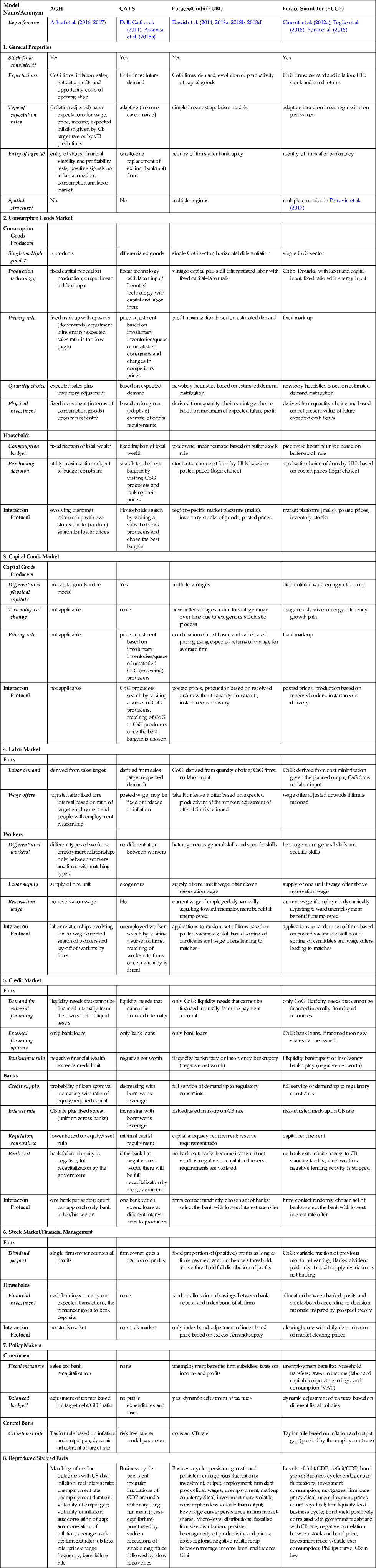
Table A2
Overview over agent-based macroeconomic models (Part 2)
| Model Name/Acronym | JAMEL | Keynes meeting Schumpeter (KS) | LAGOM | LEN |
|---|---|---|---|---|
| Key References | Seppecher (2012), Seppecher and Salle (2015), Seppecher et al. (2018) | Dosi et al. (2010, 2013, 2015, 2017c) | Wolf et al. (2013), Mandel et al. (2010) | Lengnick (2013) |
| 1. General Properties | ||||
| Stock-flow consistent? | Yes | not reported | Yes | Yes |
| Expectations | demand (all firms); leverage target (CoG) and consumption budget (HH) | CoG firms: demand | CoG firms: demand; HHs: income | CoG firms: demand |
| Type of expectation rules | naive expectations; Seppecher and Salle (2015): evolving sentiments | naive expectations | simple linear extrapolation models | naive expectations |
| Entry of agents? | firm entry only as replacement for exited firms | firm entry only as replacement for exited firms | entry/exit of firms in a sector if average profit rate is above/below average interest rate plus a risk premium | No |
| Spatial structure? | No | No | No | Yes (regional version) |
| 2. Consumption Goods Market | ||||
| Consumption Goods Producers | ||||
| Single/multiple goods? | single CoGood | single CoGood | multiple goods (identified with sectors of production) | single CoGood |
| Production technology | homogeneous capital and labor with fixed capital/labor ratio | vintage capital plus labor with fixed capital–labor ratio | Production functions. Different types available: CES, Cobb–Douglas, Leontieff | linear, labor as single input |
| Pricing rule | price adjustment if inventory is below/above target level and last period production has/has not been fully sold; Seppecher et al. (2018): evolving mark-up adjustment | mark-ups evolving based on firms' market share | mark-up over costs with mark-up rate following evolution dynamics | dynamic adjustment based on ratio of inventory and expected demand |
| Quantity choice | implied by size of labor force | proportional to expected demand taking into account current inventory | expected demand | implied by size of labor force |
| Physical investment | only Seppecher et al. (2018): derived from past sales based on NPV calculations and leverage target | derived from quantity choice plus replacement inventory (technical obsolescence); vintage choice based on price and induced prod. costs | derived from quantity choice: investment at a fixed rate whenever capacity utilization rate passes a threshold | no physical capital in the model |
| Households | ||||
| Consumption budget | buffer-stock rule | HHs every period consume their entire income | Deaton rule: save/unsave if income is greater/smaller than expected | concave function of wealth |
| Purchasing decision | cheapest observed price | not applicable (only single CoG) | allocation across sectors based on (evolving) expenditure weighs; for each good cheapest available price is selected | HHs purchase from randomly selected firm in their network |
| Interaction Protocol | firms post prices; HHs observe randomly selected group of offers | no explicit interaction protocol; market shares of firms determined by prices and unfilled demand in the previous period | HHs order firms according to price and visit them till demand is fulfilled | evolving network of connections between HHs and CoG firms based on price and unfilled demand |
| 3. Capital Goods Market | ||||
| Capital Goods Producers | ||||
| Differentiated physical capital? | homogeneous capital (in each sector) | multiple vintages | differentiated capital | no capital goods in the model |
| Technological change | no endogenous technological change; only in Seppecher et al. (2018): exogenous technological shocks | competing CaG firms update their offered vintage through innovation and imitation, process modeled in the spirit of Nelson and Winter (1982) | endogenous (at the sectoral level) | not applicable |
| Pricing rule | only in Seppecher et al. (2018): evolutionary adjustment of mark-ups | fixed mark-up | mark-up over costs with mark-up rate following evolutionary dynamics | not applicable |
| Interaction Protocol | only in Seppecher et al. (2018): capital goods firms post prices, investing firms observe randomly selected group of offers | production based on received orders, potential friction due to labor market rationing, delivery after one period | delivered upon orders based on expected demand; no frictions | not applicable |
| 4. Labor Market | ||||
| Firms | ||||
| Labor demand | adjustment relative to current labor force with a probability depending on the gap between inventory and inventory target level | CoG + CaG: derived from quantity choice | based on expected demand and minimum ratio between labor and capital | dynamic adjustment based on ratio of inventory and expected demand |
| Wage offers | adjustment of wage offer based on difference between vacancies and target vacancy rate | homogeneous wage in the economy, adjusted over time based on average productivity, inflation, unemployment | reference wage at the sectoral level evolves according to productivity; firm wage adjusted according to share of vacancies filled | adjusted upwards if firm is rationed; adjusted downwards if all positions have been filled for several periods |
| Workers | ||||
| Differentiated workers? | no differentiation between workers | no differentiation between workers | no differentiation between workers | no differentiation between workers |
| Labor supply | supply of one unit if wage offer above reservation wage | aggregate labor supply is exogenous and inelastic | supply of one unit if wage offer above reservation wage | supply of one unit |
| Reservation wage | current wage if employed; if unemployed downward adjustment with a probability that increases with duration of unemployment | not applicable | constant, randomly chosen | if employed equal to maximum of current wage and previous reservation wage; decreased if unemployed |
| Interaction Protocol | firms post wage offers; unemployed worker chooses highest wage offer within randomly selected group of observed offers, if above reservation wage | no explicit interaction protocol; rationing of firms/unemployment if labor supply differs from demand; in Dosi et al. (2017c): decentralized labor market with random matching, where firms make offers first to applicants with lowest requested wage | firms access the labor market in a random order and workers with lowest reservation wages are employed first | workers approach randomly chosen firm, if firm has vacancy worker accepts if offered wage above reservation wage |
| 5. Credit Market | ||||
| Firms | ||||
| Demand for external financing | liquidity needs that cannot be internally financed; in Seppecher et al. (2018): also long term loans as a fraction of investment costs | liquidity needs that cannot be financed internally from the own stock of liquid assets | liquidity needs that cannot be financed internally from the own stock of liquid assets (deficit computed at the end of the period) | no credit market |
| External financing options | only bank credit | only bank credit | only bank credit | not applicable |
| Bankruptcy/exit rule | inability to pay off a loan; in Seppecher et al. (2018): liabilities exceed assets | CoG and CaG: firms with near-zero market shares and/or negative net liquid assets | firm exit if profit rate below average interest rate | no bankruptcies; automatic wage cuts to keep liquidity nonnegative |
| Banks | ||||
| Credit supply | all credit demands are satisfied | supply to firms based on ranking w.r.t. liquidity/sales ratio up to (bank specific) upper bound on credit | all credit demands are satisfied | not applicable |
| Interest rate | fixed interest rate, increased if extension of due date is needed by firm | Dosi et al. (2013): fixed mark-up on CB rate; Dosi et al. (2015): risk-adjusted mark-up on CB rate | Taylor rule (one interest rate for the financial sector) | not applicable |
| Regulatory constraints | none | Dosi et al. (2013): global upper bound on credit proportional to previous period total deposits; Dosi et al. (2015): bank specific upper bound based on deposits and bad debt | none | not applicable |
| Bank exit | single bank; exit if insolvent | bank failure if net worth becomes negative; automatic bailout by the government (only Dosi et al., 2015) | only financial sector as a whole considered | not applicable |
| Interaction Protocol | single bank accommodates all requests | Dosi et al. (2013): single bank; Dosi et al. (2015): fixed firm–bank network | financial sector accommodates all requests | not applicable |
| 6. Stock Market/Financial Management | ||||
| Firms | ||||
| Dividend payout | difference between target level of net wealth (derived from leverage target) and actual net wealth (if positive) constrained by available cash-at-hand | no firm dividends | fixed dividend rate; distributed only if no debt | profits net of liqidity buffer distributed to HHs proportional to HHs liquidity |
| Households | ||||
| Financial investment | all savings kept in cash | no HH savings | only savings accounts receiving interests | all savings kept in cash |
| Interaction Protocol | no stock market | not applicable | no stock market | no stock market |
| 7. Policy Makers | ||||
| Government | ||||
| Fiscal measures | no fiscal measures | unemployment benefits, taxes on income, and profits | unemployment benefits, taxes on income | no fiscal measures |
| Balanced budget? | not applicable | fixed rates for taxes, subsidies, and unemployment benefits and endogenously evolving government deficit | yes, dynamic adjustment of tax rates | not applicable |
| Central Bank | ||||
| CB interest rate | Seppecher et al. (2018): Taylor rule (implemented by unique bank representing the whole banking sector) | Dosi et al. (2013): fixed CB rate; Dosi et al. (2015): Taylor rule based on inflation and unemployment | Taylor rule based on inflation and unemployment gaps | no CB |
| 8. Reproduced Stylized Facts | ||||
| Business cycle: endogenous persistent fluctuations; positive correlation between consumption & output; higher volatility of output; procyclical consumption, employment, inventory change, inflation, vacancy, velocity of money; countercyclical unemployment rate and duration; Beveridge curve; Phillips curve; output autocorrelation; persistence of inflation & GDP; Micro-level distributions: firms size distribution right skewed and not normal; upper part of income distribution Pareto; average level of Gini | Business cycle: endogenous persistent fluctuations; procyclical consumption, investment, change in inventory, employment, productivity, inflation, firm debt (partially with lags); countercyclical unemployment, prices, mark-ups, bank deposits; investment more volatile than GDP; consumption less volatile than GDP; distribution of aggregate growth rates with fat tails; micro-level distributions: firm size distribution skewed and not log-normal; firm growth rate distribution tent-shaped; persistent heterogeneity of labor productivity; Laplace distribution of productivity growth rates; power-law type distribution of bad debt at time of bankruptcy; lumpiness of investment; clustering of bankruptcies in time; fat tails of distribution of banking crises costs (relative to GDP) | endogenous growth; Business cycle: endogenous persistent fluctuations; investment more volatile than consumption | Business cycles: endogenous persistent fluctuations; correlation between output & lagged prices for different lags; Beveridge curve; Phillips curve; micro-level distributions: firms size distribution right skewed; right skewed distribution of frequency of price change | |
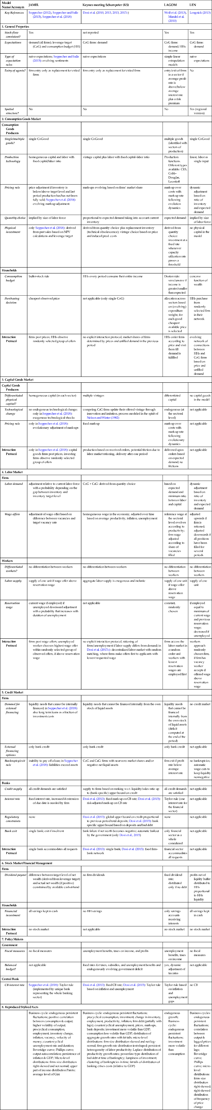
Appendix B List of Symbols
| Symbol | Meaning |
|---|---|
| C h | total consumption of household h |
| Y h | income of household h |
| S h | saving of household h |
| C i,h | consumption of variety i by household h |
| C | total households' consumption |
| C i | households' demand for variety i |
|
|
expected demand for variety i |
| Y i | output of the ith C-firm |
| Y k | output of the kth K-firm |
| J k | demand for the kth K-good |
| K i | physical capital of firm i |
| I i | investment of firm i |
| E i | net worth or equity of firm i |
| π i | profit of firm i |
| ω i | capacity utilization of firm i |
| N i | employment at firm i |
| L i | bank loans received by firm i |
|
|
desired or optimal output of firm i |
| Y | total output/income (GDP) |
| M C i | marginal cost of firm i |
| A C i | average cost of firm i |
| Q i | sales of firm i |
| Δi | inventories of firm i |
| α | marginal productivity of labor |
| F c | number of C-goods and of C-firms |
| F k | number of K-goods and of K-firms |
| F | total number of firms |
| H | total number of households |
|
|
permanent income of household h |
|
|
average income of household h |
|
|
cut-off value of the average income of household h |
| R = 1 + r | gross nominal interest rate |
|
|
human capital of household h |
|
|
financial wealth of household h |
| M h | money balances of household h |
| w h | reservation wage of household h |
| w i | wage posted by firm i |
| Symbol | Meaning |
|---|---|
| w | wage |
| P i | price of the ith C-good |
| P k | price of the kth K-good |
| P | general price level |
| p i | relative price of the ith variety |
| y i | output-to-loan ratio of firm i |
| π | inflation rate |
| k h | capitalization factor (in AGH) |
| ξ | memory parameter in permanent income algorithm (AGH) |
| δ | desired inventory-to-sale ratio |
| β | exponent of capital in the production function |
| ω f | desired wealth-to-income ratio |
| χ | parameter of quasi-replication dynamics of market share (KS) |
| v | parameter of mark-up dynamics (KS) |
| ζ1,ζ2 | parameters of competitiveness equation (KS) |
| Ωi | information set of firm i |
| e i | forecasting error of firm i |
|
|
fraction of sampled household that would good i at the price |
| λ i | leverage of firm i |
|
|
target leverage of firm i |
| μ i | mark-up of firm i |
| ν | velocity of adjustment of wealth to targeted wealth (EUBI) |
| ε | price elasticity of demand |
| ε i | price elasticity of demand expected/estimated by firm i |
|
|
total consumption expenditure estimated/expected by firm i |
| η | stochastic rate of change of the price set by each firm |
| η w | stochastic rate of change of the wage posted by each firm |
| η h | stochastic rate of change of the reservation wage |
|
|
duration of the unemployment spell (JAMEL) |
|
|
cut-off value of the unemployment spell (JAMEL) |
| Symbol | Meaning |
|---|---|
| γ | intensity of (price) competition among C-firms (EUBI) |
| ρ | intensity of adjustment of output to changes in inventories (ADG) |
| c h | propensity to consume out of human capital |
| c f | propensity to consume out of financial wealth |
| c y | propensity to consume out of income |
| f i | market share of firm i (KS) |
| E i | competitiveness of firm i (KS) |
|
|
average competitiveness of C-firms (KS) |
| s H | propensity to save when optimist (JAMEL) |
| s L | propensity to save when pessimist (JAMEL) |
| π m | probability of adopting the consumer sentiment of the majority (JAMEL) |
| π s | probability of searching for a job if unemployed (AGH) |
| π T | inflation target of the central bank (AGH) |
| v | vintage of a machine tool |
| V | total number of vintages of a machine tool |
| Z c | number of C-firms visited by a household to buy C-goods |
| Z k | number of K-firms visited by a C-firm to buy a machine tool |
| Z e | number of firms visited by a household searching for a job |