
Empirical Validation of Agent-Based Models✶
Thomas Lux⁎,1; Remco C.J. Zwinkels† ⁎Christian Albrechts Universität zu Kiel, Germany
†Vrije Universiteit Amsterdam and Tinbergen Institute, The Netherlands
1Corresponding author. email address: [email protected]
Abstract
The literature on agent-based models has been highly successful in replicating many stylized facts of financial and macroeconomic time series. Over the past decade, however, also advances in the estimation of such models have been made. Due to the inherent heterogeneity of agents and nonlinearity of agent-based models, fundamental choices have to be made to take the models to the data. In this chapter we provide an overview of the current literature on the empirical validation of agent-based models. We discuss potential lessons from other fields of applications of agent-based models, avenues for estimation of reduced form and ‘full-fledged’ agent-based models, estimation methods, as well as applications and results.
Keywords
Agent-based models; Validation; Method of moments; State space models; Sequential Monte Carlo; Switching mechanisms; Reduced form models
1 Introduction
The primary field of development of agent-based models in economics has been the theory of price formation in financial markets. It is also in this area that we find the vast majority of attempts in recent literature to develop methods for estimation of such models. This is not an accidental development. It is rather motivated by the particular set of ‘stylized facts’ observed in financial markets. These are overall statistical regularities characterizing asset returns and volatility, and they seem to be best understood as emergent properties of a system composed of dispersed activity with conflicting centrifugal and centripetal tendencies. Indeed, ‘mainstream’ finance has never even attempted an explanation of these stylized facts, but often has labeled them ‘anomalies’. In stark contrast, agent-based models seem to be generically able to relatively easily replicate and explain these stylized facts as the outcome of market interactions of heterogeneous agents.
The salient characteristics of the dynamics of asset prices are different from those of dynamic processes observed outside economics and finance, but are surprisingly uniform across markets. There are highly powerful tools available to quantify these dynamics, such as GARCH models to describe time-varying volatility (see Engle and Bollerslev, 1986) and Extreme Value Theory to quantify the heaviness of the tails of the distribution of asset returns (see e.g. Embrechts et al., 1997). For a long time very little has been known about the economic mechanisms causing these dynamics. The traditional paradigm building on agent rationality and consequently also agent homogeneity has not been able to provide a satisfying explanation for these complex dynamics. This lack of empirical support coupled with the unrealistic assumptions of the neoclassical approach has contributed to the introduction and rise of agent-based models (ABMs) in economics and finance; see e.g. Arthur (2006) in the previous edition of this handbook.
Whereas the strength of ABMs is certainly their ability to generate all sorts of complex dynamics, their relatively (computationally) demanding nature is a drawback. This was, among others, a reason why Heterogeneous Agent Models (HAMs) were developed as a specific type of agent based models. Most HAMs only consider two very simple types of agents. Specifically, most models contain a group of fundamentalists expecting mean reversion and chartists expecting trend continuation. The main source of dynamics, however, is a switching function allowing agents to switch between the two groups conditional on past performance. Interestingly, even such simplified and stylized versions of ABMs are capable of replicating the complex price dynamics of financial markets to a certain degree; see e.g. Hommes (2006) for an overview. Recent research has also collected catalogs of stylized facts of macroeconomic data, and agent-based approaches have been developed to explain those (e.g. Dosi et al., 2013, 2015).
Due to the aforementioned background of ABMs, the early literature has typically been relying on simulations to study the properties of models with interacting agents. By doing so, authors were able to illustrate the ability of ABMs to generate complex dynamic processes resembling those observed in financial markets. There are, however, several good reasons why especially ABMs should be confronted with empirical data. First of all, ABMs are built on the notion of bounded rationality. This generates a large number of degrees of freedom for the theorist as deviations from rationality can take many forms. Empirical verification of the choices made in building the models can therefore enforce discipline in model design. Second, by confronting ABMs with empirical data, one should get a better understanding of the actual law of motion generating market prices. Whereas simulation exercises with various configurations might generate similar dynamics, a confrontation with empirical data might allow inference on relative goodness-of-fit in comparison to alternative explanations. This is especially appealing because the introduction of ABMs was empirically motivated in the first place. Finally, empirical studies might allow agent based models to become more closely connected to the ‘mainstream’ economics and finance literature. Interestingly, certain elements underlying ABMs have been used in more conventional settings; see for example Cutler et al. (1991) or Barberis and Shleifer (2003), who also introduce models with boundedly rational and interacting agents. Connections between these streams of literature, however, are virtually non-existent. By moving on to empirical validation, which could also serve as a stepping stone towards more concrete applications and (policy) recommendations, the ABM literature should become of interest and relevance to a broader readership.
While ABMs are based on the behavior of and interaction between individual agents, they typically aspire to explain macroscopic outcomes and therefore most empirical studies are also focusing on the market level. The agent based approach, however, by definition has at its root the behavior of individual agents and, by doing so, any ABM necessarily makes a number of assumptions about individual behavior. Stepping away from the rational representative agent approach implies that alternative behavioral assumptions have to be formulated. Whereas rational behavior is uniquely defined, boundedly rational behavior can take many forms. Think, for example, of the infinite number of subsets that can be extracted from the full information set relevant for investing, let alone the sentiment that agents might incorporate in their expectations. To address these two issues, Hong and Stein (1999) define three criteria the new paradigm should adhere to, which serve as a devise to restrict the modeler's imagination. The candidate theory should (i) rest on assumptions about investor behavior that are either a-priori plausible or consistent with casual observation; (ii) explain the existing evidence in a parsimonious and unified way; and (iii) make a number of further predictions that can be subject to out-of-sample testing. Whereas empirical evidence at the macro-level mainly focuses on criteria (ii) and (iii), micro-level evidence is necessary to fulfill criterion (i) and thereby find support for the assumptions made in building the agent based models. This is especially pressing for the reduced form models discussed in Section 3, as a number of assumptions are made for example regarding the exact functional form of the heterogeneous groups.
Taking ABMs to the data is not straightforward due to an often large number of unknown parameters, nonlinearity of the models leading to a possibly non-monotonic likelihood surface, and sometimes limited data availability. As such, one needs to make choices in order to be able to draw empirical inferences. In this review, we distinguish between two approaches. The first approach covers (further) simplifications of ABMs and HAMs to reduced form models making them suitable for estimation using relatively standard econometric techniques. These reduced form models are often sufficiently close to existing econometric models, with the additional benefit of a behavioral economic underpinning. The second approach is less stringent in the additional assumptions made on agent behavior, but requires more advanced estimation methods. Typically, these methods belong to the class of simulation-based estimators providing the additional benefit that the model is not fitted on the mean of the data, as typically is the case when using standard estimation techniques, but on the (higher) moments. This creates a tighter link between the original purpose of ABMs of explaining market dynamics and the empirical approach.
All in all, the empirical literature on agent based models has been mounting over the past decade. There have been interesting advances in terms of methods, models, aggregation approaches, as well as markets, which we will review in this chapter. The empirical results generally appear to be supportive of the agent-based approach, with an emphasis on the importance of dynamics in the composition of market participants. The estimation methods and exact functional forms of groups of agents vary considerably across studies, making it hard to draw general conclusions and to compare results across studies. The common denominator, however, is that virtually all studies find evidence in support of the relevance of the heterogeneity of agents. Allowing agents to switch between groups generally has a positive effect on model fit. These results typically hold both in-sample and out-of-sample. In view of the dominance of financial market applications of agent-based models, most of this survey will be dealing with attempts at estimating ABMs designed to explain asset price dynamics. We note, however, that the boundaries between agent-based models and more traditional approaches are becoming more and more fuzzy. For example, recent dynamic game-theoretic and microeconomic models (Blevins, 2016; Gallant et al., 2016) also entail a framework of a possibly heterogeneous pool of agents interacting in a dynamic setting. Similarly, heterogeneity has been allowed for in standard macroeconomic models in various ways (e.g., Achdou et al., 2015). However, all these approaches are based on inductive solutions of the agents' optimization problem while models that come along with the acronym ABM would typically assume some form of bounded rationality. We stick to this convention and mainly confine attention to ABMs with some kind of boundedly rational behavior. Notwithstanding this confinement, models with a multiplicity of rational agents might give rise to similar problems and solutions when it comes to their empirical validation.
Being boundedly rational agents ourselves, this chapter no doubt suffers from the heuristics we have applied in building a structure and selecting papers. As such, this review should not be seen as an exhaustive overview of the existing literature, but rather as our idiosyncratic view of it. The remainder of the chapter is organized as follows. In Section 2 we discuss which insights economists can gain from other fields when it comes to estimation of ABMs. Whereas Section 3 discusses reduced form models, Section 4 reviews the empirical methods employed in estimation of more general variants of agent-based models. It also proposes a new avenue for estimation by means of state-space methods, which have not been applied in agent-based models in economics and finance so far. Section 5 discusses the empirical evidence for ABMs along different types of data at both the individual and the aggregate level that can be used to validate agent-based models. Section 6, finally, concludes and offers our view on the future of the field.
2 Estimation of Agent-Based Models in Other Fields
The social sciences seem to be the field predestined for the analysis of individual actors and the collective behavior of groups of them. However, agent-based modeling is not strictly confined to subjects dealing with humans, as one could, for example, also conceive of the animals or plants of one species as agents, or of different species within an ecological system. Indeed, biology is one field in which a number of potentially relevant contributions for the subject of this review can be found. Before we move on to such material, we first provide an overview over agent-based models and attempts at their validation in social sciences other than economics.
2.1 Sociology
Sociology by its very nature concerns itself with the effects of interactions of humans. In contrast to economics, there has never been a tradition like that of the ‘representative agent’ in this field. Hence, interaction among agents is key to most theories of social processes. The adaptation of agent-based models on a relatively large scale coincided with a more computational approach that has appeared over the last decades. Many of the contributions published in the Journal of Mathematical Sociology (founded in 1971) can be characterized as agent-based models of social interactions, and the same applies to the contributions to Social Networks (founded in 1979). The legacy of seminal contributions partly overlaps with those considered milestones of agent-based research in economic circles as well, e.g. Schelling's model of the involuntary dynamics of segregation processes among ethnic groups (Schelling, 1971), and Axelrod's analysis of the evolution of cooperation in repeated plays of prisoners” dilemmas (Axelrod, 1984). Macy and Willer (2002) provide a comprehensive overview over the use of agent-based models and their insights in sociological research. More recently, Bruch and Atwell (2015) and Thiele et al. (2014) discuss strategies for validation of agent-based models.
These reviews not only cover contributions in sociology alone, but also provide details on estimation algorithms applied in ecological models as well as systematic designs for confrontation of complex simulation models with data (of which agent-based models are a subset). A systematic approach to estimation of an interesting class of agent-based models has been developed in network theory. The pertinent class of models has been labeled ‘Stochastic Actor-Oriented Models’ (SAOM). It formalizes individuals' decisions to form and dissolve links to other agents within a network setting. This framework bears close similarity to models of discrete choice with social interactions in economics (Brock and Durlauf, 2001a, 2001b). The decision to form, keep or give up a link is necessarily of discrete nature. Similar to discrete choice models, the probabilities for agents to change from one state to another are formalized by multinomial logit expressions. This also allows the interpretation that the agents' objective functions contain a random idiosyncratic term following an extreme value distribution. The objective function naturally is a function evaluating the actor's satisfaction with her current position in the network. This ‘evaluation function’ is, in principle, completely flexible and allows for a variety of factors of influence on individuals' evaluation of network ties: actor-specific properties whose relevance can be evaluated by including actor covariates in the empirical analysis (e.g., male/female), dyadic characteristics of pairs of potentially connected agents (e.g., similarity with respect to some covariate), overall network characteristics (e.g., local clustering), as well as time-dependent effects like hysteresis or persistence of existing links or ‘habit formation’ (e.g., it might be harder to cut a link, the longer it has existed).
Snijders (1996) provides an overview over the SAOM framework. For estimation, various approaches have been developed: Most empirical applications use the method of moments estimator (Snijders, 2001), but recently also a Generalized Method of Moments (GMM) approach has been developed (Amati et al., 2015). Maximum likelihood estimation (Snijders et al., 2010) and Bayesian estimation (Koskinen and Snijders, 2007) are feasible as well. The set-up of the SAOM approach differs from that of discrete choice models in economics in that agents operate in a non-equilibrium setting, while the discrete choice literature usually estimates its models under rational expectations, i.e. assuming agents are operating within an equilibrium configuration correctly taking into account the influence of each agent on all other agents' utility functions. While the SAOM framework does not assume consistency of expectations, one can estimate its parameters under the assumption that the data are obtained from the stationary distribution of the underlying stochastic process. If the model explicitly includes expectations (which is typically not the case in applications in sociology) these should then have become consistent. Recent generalizations include an extension of the decision process by allowing for additional behavioral variables besides the network formation activities of agents (Snijders et al., 2007) and modeling of bipartite networks, i.e. structures consisting of two different types of agents (Koskinen and Edling, 2012). The tailor-made R package SIENA (Snijders, 2017) covers all these possibilities, and has become the work tool for a good part of sociological network research. Economic applications include the analysis of managers' job mobility on the creation of interfirm ties (Checkley and Steglich, 2007), and the analyses of link formation in the interbank money market (Zappa and Zagaglia, 2012; Finger and Lux, 2017). A very similar approach to the estimation of network models of human interactions within the context of development policy can be found in Banerjee et al. (2013).
2.2 Biology
Agent-based simulation models have found pervasive use in biology, in particular for modeling of population dynamics and ecological processes. The range of methods to be found in these areas tends to be wider than in the social sciences. In particular, various simulation-based methods of inference are widely used that have apparently hardly ever been adopted for validation of ABMs in the social sciences or in economics. Relatively recent reviews can be found in Hartig et al. (2011) and Thiele et al. (2014), who both cover ecological applications along with sociological ones. Methods used for estimation of the parameters of ecological models include Markov Chain Monte Carlo (MCMC), Sequential Monte Carlo (SMC), and particle filters, which are all closely related to each other. In most applications, the underlying model is viewed as a state-space model with one or more unobservable state(s) governed by the agent-based model and a noisy observation that allows indirect inference on the underlying states together with the estimation of the parameters of the pertinent model. In a linear, Gaussian framework for both the dynamics of the hidden state and the observation, such an inference problem can be solved most efficiently with the Kalman filter. In the presence of nonlinearities and non-Gaussianity, alternative, mostly simulation-based methods need to be used. An agent-based model governing the hidden states by its very nature typically is a highly nonlinear and non-Gaussian process, and often can only be implemented by simulating its defining microscopic laws of motion. The simulation-based methods mentioned above would then allow to numerically approximate the likelihood function (or if not available, any other objective function) via some population-based evolutionary process for the parameters and states, in which the simulation of the ABM itself is embedded.
Markov Chain Monte Carlo samples the distribution of the model's parameters within an iterative algorithm in which the next step depends on the likelihood of the previous one. In each iteration, a proposal for the parameters is computed via a Markov Chain, and the proposal is accepted with a probability that depends on its relative likelihood vis-à-vis the previous draws and their relative probabilities to be drawn in the Markov chain. After a certain transient this chain should converge to the stationary distribution of the parameters allowing to infer their expectations and standard errors. In Sequential Monte Carlo, it is not one realization of parameters, but a set of sampled realizations that are propagated through a number of intermediate steps to the final approximation of the stationary distribution of the parameters (cf. Hartig et al., 2011). In an agent-based (or population-based) framework, the simulation of the unobservable part (the agent-based part) is often embedded via a so-called particle filter in the MCMC or SMC framework. Proposed first by Gorden et al. (1993) and Kitagawa (1996), the particle filter approximates the likelihood of a state-space model by a swarm of ‘particles’ (possible realizations of the state) that are propagated through the state and observation parts of the system. Approximating the likelihood by the discrete probability function summarizing the likelihood of the particles, one can perform either classical inference or use the approximations of the likelihood as input in a Bayesian MCMC or SMC approach.
Advanced particle methods use particles simultaneously for the state and the parameters (Kitagawa, 1998). With the augmented state vector, filtering and estimation would be executed at the same time, and the surviving particles of the parameters at the end of one run of this so-called ‘auxiliary’ particle filter would be interpreted as parameter estimates. Instructive examples from a relatively large pertinent literature in ecology include Golightly and Wilkinson (2011), who estimate the parameters of partly observed predator-prey systems via Markov Chain Monte Carlo together with a particle filter of the state dynamics, or Ionides et al. (2006), who apply frequentist maximum likelihood based on a particle filter to epidemiological data. MCMC methods have also been applied for rigorous estimation of the parameters of traffic network models, cf. Molina et al. (2005). An interesting recent development is Approximate Bayesian Computation (ABC) that allows inference based on MCMC and SMC algorithms using objective functions other than the likelihood (Sisson et al., 2005; Toni et al., 2008). Since it is likely that for ABMs of a certain complexity, it will not be straightforward to evaluate the likelihood function, these methods should provide a welcome addition to the available toolbox.
2.3 Other Fields
Agent-based models can be viewed as a subset of ‘computer models’, i.e., models with an ensemble of mathematical regularities that can only be implemented numerically. Such models might not have units that can be represented as agents, but might take the form of large systems of complex (partial) differential equations. Examples are various models of industrial processes (cf. Bayarri et al., 2007), or the fluid dynamical systems used in climate change models (Stephenson et al., 2012). In biology, one might, in fact, sometimes have the choice to use an agent-based representation of a certain model, or rather a macroscopic approximation using, for example, a low-dimensional system of differential equations (cf. Golightly et al., 2015, for such an approach in an ecological model). Similar approximation of agent-based models in economics can be found in Lux (2009a, 2009b, 2012). The same choice might be available for other agent-based models in economics or finance (see below Section 4.3). In macroeconomics, dynamic stochastic general equilibrium (DSGE) models are medium-sized systems of non-linear difference equations that have also been estimated in recent literature via Markov Chain Monte Carlo and related methods (e.g., Amisano and Tristani, 2010).
In climate modeling, epidemics (Epstein, 2009), and industrial applications (Bayarri et al., 2007), models have become so complex that an estimation of the complete model often becomes unfeasible. The same applies to computational models in anthropology such as the well-known model of Anasazi settlement dynamics in northeastern Arizona (Axtell et al., 2002). The complexity of such models also implies that only a limited number of scenarios can be simulated and that different models can at best be compared indirectly. The epistemological consequences of this scenario are intensively discussed in climate change research as well as in the social sciences (cf. Carley and Louie, 2008). In the context of very complex models and/or sparse data, empirical validation is often interpreted in a broader sense than estimation proper. Aiming to replicate key regularities of certain data is known in ecology as pattern-oriented modeling (cf. Grimm et al., 2005). This is equivalent to what one would call ‘matching the stylized facts’ in economics. As far as patterns can be summarized as functions of the data and a simulated agent-based model could be replicated without too much computational effort, a more rigorous version of pattern-oriented modeling would consist in a method-of-moments approach based upon the relevant patterns. However, even if only a small number of simulations of a complex simulation model can be run, estimation of parameters through rigorous exploitation of the (scarce) available information is possible. Within the framework of industrial applications and epidemiological dynamics, Bayarri et al. (2007), Higdon et al. (2008), and Wang et al. (2009) provide a systematic framework for a Bayesian estimation approach that corrects the biases and assesses the uncertainties inherent in large simulation models that can neither be replicated often nor selectively modified. In the analysis of complex models of which only a few replications are available often so-called emulation methods are adopted to construct a complete response of model output on parameters. Typically, emulator functions make use of Gaussian processes and principal component analysis (e.g., Hooten and Wikle, 2010; Heard, 2014; Rasouli and Timmermans, 2013). One might envisage that such a framework could also be useful for macroeconomics once agent-based models of various economic spheres are combined into larger models.
3 Reduced Form Models
The literature on agent-based models was initially purely theoretical in nature. As such, the benchmark models did not take the restrictions into account that empirical applications require. A number of issues in the theoretical models need to be addressed before the models can be confronted with empirical data, especially when focusing on market level studies. One direction is to use advanced econometric techniques, which we will discuss in Section 4. Another direction is to rewrite the model in a reduced form. Bringing HAMs to the data introduces a trade-off between the degree of micro-foundation of the (empirical) model and the appropriateness of the model for estimation. A first choice is the form of the dependent (endogenous) variable. Several models, such as, for example, Day and Huang (1990) and Brock and Hommes (1997), are written in terms of price levels. This poses no problems in an analytical or simulation setting, but could become problematic when turning to calibration or estimation. Most standard econometric techniques assume that the input data is stationary. This assumption, however, is typically violated when using financial prices or macroeconomic time series.
The second issue is the identification of coefficients. The theoretical models contain coefficients that might not all be identified econometrically, which means that one could not obtain an estimate of all the behavioral parameters of a model but that, for instance, only composite expressions of the primitive parameters can be estimated. A third issue relates to the switching mechanism that is typically applied in HAMs. Allowing agents to switch between strategies is, perhaps, the identifying characteristic of HAMs and an important source of dynamics in simulation settings. At the same time it poses a challenge for empirical work, as the switching function is by definition non-linear which could create a non-monotonic likelihood surface.
A final issue we want to discuss here, is the choice of the fundamental value in asset-pricing applications. The notion of a fundamental value is intuitively appealing and central to the behavior of ‘fundamentalists’ in HAMs. Empirically, though, the ‘true’ fundamental value is principally unobservable. As there is no objective choice for the fundamental value, any estimation of a model including a fundamental value will therefore inevitably suffer from the ‘joint hypothesis problem’, cf. Fama (1991). We will discuss these four issues in more detail in the following subsections.
3.1 Choice of Dependent Variable
Whereas several HAMs are principally written in terms of price levels, empirical studies using market data are hardly ever based on price levels due to the non-stationarity issue. Possible solutions to this issue include working with alternative econometric methods, such as, e.g., cointegration techniques (Amilon, 2008; Frijns and Zwinkels, 2016a, 2016b) or simulation techniques (Franke, 2009; Franke and Westerhoff, 2011), but the more typical solution is to reformulate the original model such that the left hand side variable is stationary.
Two main approaches consist of empirical models in terms of returns, ΔPt=Pt−Pt−1![]() with Pt
with Pt![]() the asset price at time t, and empirical models in terms of price deviation from the fundamental, Pt−P⁎t
the asset price at time t, and empirical models in terms of price deviation from the fundamental, Pt−P⁎t![]() . The choice between the two is driven by the underlying HAM, or more specifically its micro-foundation and market clearing mechanism.1 Micro-founded equilibrium models based on a Walrasian auctioneer, such as Brock and Hommes (1997, 1998), assume the existence of an all-knowing auctioneer who collects all supply and demand schedules and calculates the market clearing price. These models are typically written in terms of price levels. It is not possible to convert these into price changes because prices are modeled as a non-linear function of lagged prices. Disequilibrium models based on the notion of a market maker, see Beja and Goldman (1980), Day and Huang (1990), or Chiarella (1992) for early examples, assume that net demand (supply) causes prices to increase (decrease) proportionally, without assuming market clearing. These models are typically written in terms of price changes or are easily reformulated as such.2
. The choice between the two is driven by the underlying HAM, or more specifically its micro-foundation and market clearing mechanism.1 Micro-founded equilibrium models based on a Walrasian auctioneer, such as Brock and Hommes (1997, 1998), assume the existence of an all-knowing auctioneer who collects all supply and demand schedules and calculates the market clearing price. These models are typically written in terms of price levels. It is not possible to convert these into price changes because prices are modeled as a non-linear function of lagged prices. Disequilibrium models based on the notion of a market maker, see Beja and Goldman (1980), Day and Huang (1990), or Chiarella (1992) for early examples, assume that net demand (supply) causes prices to increase (decrease) proportionally, without assuming market clearing. These models are typically written in terms of price changes or are easily reformulated as such.2
The most widely applied configuration is the model with a market maker in terms of price changes or returns (see e.g. Frankel and Froot, 1990; Reitz and Westerhoff, 2003; Reitz et al., 2006; Manzan and Westerhoff, 2007; De Jong et al., 2009, 2010; Kouwenberg and Zwinkels, 2014, 2015). The empirical models are typically of the form:
(1) ΔPt=c+wftα(Pt−1−P⁎t−1)+wctβΔPt−1+εt
in which wft![]() and wct
and wct![]() are the fundamentalist and chartist weights, respectively, εt
are the fundamentalist and chartist weights, respectively, εt![]() is the noise factor and c, α, and β are the coefficients to be estimated. Given that both the left hand and right hand side variables are denoted in differences, the stationarity issue is largely extenuated. At the same time, there is no (explicit) micro-foundation in the sense of a utility or profit maximizing framework that motivates the behavior of the two groups of agents in this model.
is the noise factor and c, α, and β are the coefficients to be estimated. Given that both the left hand and right hand side variables are denoted in differences, the stationarity issue is largely extenuated. At the same time, there is no (explicit) micro-foundation in the sense of a utility or profit maximizing framework that motivates the behavior of the two groups of agents in this model.
In a series of papers, Alfarano et al. (2005, 2006, 2007) set up a HAM with trading among speculators and a market maker that results in a dynamic process for log returns. They derive a closed-form solution for the distribution of returns that is conditional on the structural parameters of the model and estimate these parameters via an approximate maximum likelihood approach. In a follow-up study, Alfarano et al. (2008) derive closed form solutions to the higher moments of the distribution.
The second approach is to write the model in terms of price deviations from the fundamental value, xt=Pt−P⁎t![]() , or a variant thereof. The implicit assumption that is made, is that the price and fundamental price are cointegrated with cointegrating vector (1,−1)
, or a variant thereof. The implicit assumption that is made, is that the price and fundamental price are cointegrated with cointegrating vector (1,−1)![]() , such that the simple difference between the two is stationary.3 One example of this approach is Boswijk et al. (2007), who initially base their study on the Brock and Hommes (1998) model in terms of price levels:
, such that the simple difference between the two is stationary.3 One example of this approach is Boswijk et al. (2007), who initially base their study on the Brock and Hommes (1998) model in terms of price levels:
(2) Pt=11+rH∑h=1nh,tEh,t(Pt+1+yt+1),

with Eh,t(⋅)![]() denoting the expectation of agents of group h, nh,t
denoting the expectation of agents of group h, nh,t![]() their number at time t, yt
their number at time t, yt![]() the dividend and r the risk-free interest rate. Dividing the left and right-hand side of Eq. (1) by dividend yt
the dividend and r the risk-free interest rate. Dividing the left and right-hand side of Eq. (1) by dividend yt![]() and assuming that yt+1=(1+g)yt
and assuming that yt+1=(1+g)yt![]() , Eq. (2) can be written in terms of price-to-cash flow
, Eq. (2) can be written in terms of price-to-cash flow
(3) δt=1R⁎{1+H∑h=1nh,tEh,t(δt+1)}
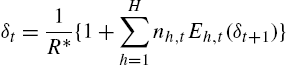
in which δ=Pt/yt![]() and R⁎=(1+g)/(1+r)
and R⁎=(1+g)/(1+r)![]() . Assuming a fundamental value based on the Gordon growth model, the fundamental is given by P⁎t=1+gr−gyt
. Assuming a fundamental value based on the Gordon growth model, the fundamental is given by P⁎t=1+gr−gyt![]() , such that the fundamental price-to-cash-flow ratio is given by δ⁎t=1+gr−g
, such that the fundamental price-to-cash-flow ratio is given by δ⁎t=1+gr−g![]() . Finally, Boswijk et al. (2007) use xt=δt−δ⁎t
. Finally, Boswijk et al. (2007) use xt=δt−δ⁎t![]() as the input to their empirical model. This approach has been applied, among others, by Chiarella et al. (2014).
as the input to their empirical model. This approach has been applied, among others, by Chiarella et al. (2014).
Clearly, the choice of model has consequences on the results but also on the interpretation of the results. The deviation type models assume that xt![]() is the variable that investors form expectations about, whereas the return type models assume that ΔPt
is the variable that investors form expectations about, whereas the return type models assume that ΔPt![]() is the variable that investors form expectations about. Theoretically these should be equivalent, but we know from social psychology that people respond differently to such different representations of the same information. For example, Glaser et al. (2007) find in an experimental study that price forecasts tend to have a stronger mean reversion pattern than return forecasts. Furthermore, in the deviation type models the two groups of agents rely on the same type of information, namely xt−1
is the variable that investors form expectations about. Theoretically these should be equivalent, but we know from social psychology that people respond differently to such different representations of the same information. For example, Glaser et al. (2007) find in an experimental study that price forecasts tend to have a stronger mean reversion pattern than return forecasts. Furthermore, in the deviation type models the two groups of agents rely on the same type of information, namely xt−1![]() or last period's price deviation. Fundamentalism and chartism are subsequently distinguished by the coefficients in the expectations function, in which a coefficient >1 (<1) implies chartism (fundamentalism). This interpretation, however, is not exactly the same as with the original models of fundamentalists and chartists because chartists do not expect a price trend to continue but rather expect the price deviation from fundamental to increase. Furthermore, this setup is rather restrictive in that it does not allow for the inclusion of additional trader types. In the return based models, on the other hand, agents use different information sets as indicated in Eq. (1). This allows for more flexibility as any trader type can be added to the system. De Jong et al. (2009), for example, include a third group of agents to their model, internationalists, next to fundamentalists and chartists.
or last period's price deviation. Fundamentalism and chartism are subsequently distinguished by the coefficients in the expectations function, in which a coefficient >1 (<1) implies chartism (fundamentalism). This interpretation, however, is not exactly the same as with the original models of fundamentalists and chartists because chartists do not expect a price trend to continue but rather expect the price deviation from fundamental to increase. Furthermore, this setup is rather restrictive in that it does not allow for the inclusion of additional trader types. In the return based models, on the other hand, agents use different information sets as indicated in Eq. (1). This allows for more flexibility as any trader type can be added to the system. De Jong et al. (2009), for example, include a third group of agents to their model, internationalists, next to fundamentalists and chartists.
There is also an important econometric difference between the deviation and return type models. In the deviation type models, the two groups are not identified under the null of no switching because both rely exclusively on xt−1![]() as information; the switching parameter is a nuisance parameter; see Teräsvirta (1994). As a result, the statistical added value of switching is to be determined using a bootstrap procedure. In the return-based models, however, this issue does not hold as both groups remain identified under the null of no switching, and the added value of switching is therefore determined by means of standard goodness-of-fit comparisons.4
as information; the switching parameter is a nuisance parameter; see Teräsvirta (1994). As a result, the statistical added value of switching is to be determined using a bootstrap procedure. In the return-based models, however, this issue does not hold as both groups remain identified under the null of no switching, and the added value of switching is therefore determined by means of standard goodness-of-fit comparisons.4
3.2 Identification
The original HAMs have a relatively large number of parameters, which might not all be identified in an estimation setting. As a result, the econometrician will have to make one or more simplifying assumptions such that all parameters are identified. As in the previous subsection, here we can also make the distinction between models based on a Walrasian auctioneer and models based on a market maker.
Brock and Hommes (1997) build their model using mean-variance utility functions, resulting in a demand function of group h of the form
(4) zht=Eht(Pt+1+yt+1−RPt)ahσ2
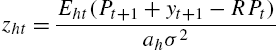
in which R=1+r![]() , a is the coefficient of risk aversion, and σ market volatility. Now assume a very simple structure of the expectation formation rule:
, a is the coefficient of risk aversion, and σ market volatility. Now assume a very simple structure of the expectation formation rule:
(5) Eht(Pt+1+yt+1−RPt)=αh(Pt−1+yt−1−RPt−2)
such that
(6) zht=αh(Pt−1+yt−1−RPt−2)ahσ2.
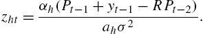
The empirical issue with such a demand function, is that the coefficients ah![]() and αh
and αh![]() cannot be distinguished from each other. One solution is to take α′h=αh/ahσ2
cannot be distinguished from each other. One solution is to take α′h=αh/ahσ2![]() , assuming volatility is constant such that α′h
, assuming volatility is constant such that α′h![]() is also a constant that can be estimated. This assumption, however, is at odds with the initial motivation of HAMs to provide an economic explanation for time-varying volatility. Therefore, the following steps are typically taken. Summing up the demand functions over groups and equating to supply yields the market clearing condition:
is also a constant that can be estimated. This assumption, however, is at odds with the initial motivation of HAMs to provide an economic explanation for time-varying volatility. Therefore, the following steps are typically taken. Summing up the demand functions over groups and equating to supply yields the market clearing condition:
(7) ΣhnhtEht(Pt+1+yt+1−RPt)ahσ2=zst

in which nht![]() is the proportion of agents in group h in period t, and zst
is the proportion of agents in group h in period t, and zst![]() is the supply of the asset. Brock and Hommes (1997) subsequently assume a zero outside supply of stocks, zst=0
is the supply of the asset. Brock and Hommes (1997) subsequently assume a zero outside supply of stocks, zst=0![]() , such that
, such that
(8) RPt=ΣhnhtEht(Pt+1+yt+1).
In other words, by assuming zero outside supply, the risk aversion coefficients an![]() drop out of the equation and agents effectively become risk neutral provided all groups h are characterized by the same degree of risk aversion (so that groups only differ in their prediction of future price movements). This step eliminates the identification issue, but also reduces the impact of agent's preferences on their behavior. As an alternative avenue, Hommes et al. (2005a, 2005b) introduce a market maker who adjusts the price in the presence of excess demand or excess supply.
drop out of the equation and agents effectively become risk neutral provided all groups h are characterized by the same degree of risk aversion (so that groups only differ in their prediction of future price movements). This step eliminates the identification issue, but also reduces the impact of agent's preferences on their behavior. As an alternative avenue, Hommes et al. (2005a, 2005b) introduce a market maker who adjusts the price in the presence of excess demand or excess supply.
In a setting with a market maker, authors typically start by specifying demand functions of the form
(9) Dft=αf(Pt−P⁎t),Dct=αc(Pt−Pt−1)
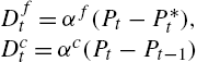
with superscripts f and c denoting the pertinent reaction coefficients of fundamentalists and chartists, respectively. Note that these are already simplified in the sense that risk preference is not taken into account. This either implies that agents are risk neutral, or that αf![]() and αc
and αc![]() can be interpreted broader as coefficients capturing both the expectation part and a risk adjustment part, αf=αf′/aσ
can be interpreted broader as coefficients capturing both the expectation part and a risk adjustment part, αf=αf′/aσ![]() . This works again under the assumption that volatility σ is constant.
. This works again under the assumption that volatility σ is constant.
Aggregating demand of the two groups yields market demand:
(10) Dmt=nftDft+nctDct
such that the price equation is given by
(11) Pt=Pt−1+λDmt+εt
in which λ is the market maker reaction coefficient, and εt![]() is a stochastic disturbance.
is a stochastic disturbance.
In this setting, the market maker reaction coefficient λ is empirically not identifiable independently of αf![]() and αc
and αc![]() . Two solutions to this issue have been proposed. Either one assumes that λ=1
. Two solutions to this issue have been proposed. Either one assumes that λ=1![]() such that the estimated coefficient equals αh
such that the estimated coefficient equals αh![]() , or one interprets the estimated coefficient as a market impact factor, equal to αhλ
, or one interprets the estimated coefficient as a market impact factor, equal to αhλ![]() . Both solutions entail that both groups have the same price elasticity of demand.
. Both solutions entail that both groups have the same price elasticity of demand.
Both solutions described here result in extremely simple models of price formation. They do, however, capture the main behavioral elements of HAMs: boundedly rational expectation formation by heterogeneous agents, consistent with empirical evidence, combined with the ability to switch between groups. In addition, simulation exercises also illustrate that certain variants of these models are still able to generate some of the main stylized facts of financial markets, such as their excess volatility and the emergence and breakdown of speculative bubbles (Day and Huang, 1990; Chiarella, 1992). The ABM character underlying these empirical models essentially represents an economic underpinning of time-varying coefficients in an otherwise quite standard econometric model capturing conditional trends and mean-reversion.
3.3 Switching Mechanism
One of the main issues in estimating ABMs follows from the non-linear nature of the model that (mainly) arises from the existence of the mechanism that governs the switching between beliefs. As a result, the likelihood surface tends to be rugged making it challenging to find a global optimum. This issue has been explored either directly or indirectly by a number of papers. Several approaches have been used.
As an early example, Shiller (1984) introduces a model with rational smart money traders and ordinary investors and shows that the proportion of smart money traders varies considerably during the 1900–1983 period by assuming the aggregate effect of ordinary investors to be zero. Frankel and Froot (1986, 1990) have a very similar approach. Specifically, Frankel and Froot (1986) assume that market-wide expected returns are equal to the weighted average of fundamentalist and chartist expectations:
(12) Δsmt+1=ωtΔsft+1+(1−ωt)Δsct+1
with Δsmt+1![]() , Δsft+1
, Δsft+1![]() and Δsct+1
and Δsct+1![]() denoting the expected exchange rate changes of the overall ‘market’, of the fundamentalist group and of the chartist group, respectively, and wt
denoting the expected exchange rate changes of the overall ‘market’, of the fundamentalist group and of the chartist group, respectively, and wt![]() being the weight assigned by ‘the market’ to the fundamentalist forecast.5
being the weight assigned by ‘the market’ to the fundamentalist forecast.5
By assuming that chartists expect a zero return, we get
(13) ωt=Δsmt+1Δsft+1.
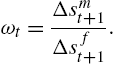
Frankel and Froot (1990) subsequently proxy Δsmt+1![]() by the forward discount, and Δsft+1
by the forward discount, and Δsft+1![]() by survey expectations. In this way, they implicitly back out the time-varying fundamentalist weight ωt
by survey expectations. In this way, they implicitly back out the time-varying fundamentalist weight ωt![]() from the data. Apart from making some strong assumptions about agent behavior, this method identifies the time-varying impact of agent groups, but does not identify the drivers of this time-variation.
from the data. Apart from making some strong assumptions about agent behavior, this method identifies the time-varying impact of agent groups, but does not identify the drivers of this time-variation.
Reitz and Westerhoff (2003) and Reitz et al. (2006) estimate a model of chartists and fundamentalists for exchange rates by assuming the weight of technical traders to be constant, and the weight of fundamental traders to depend on the normalized misalignment between the market and fundamental price. As such, there is no formal switching between forecasting rules, but the impact of fundamentalists is time-varying. Manzan and Westerhoff (2007) introduce time-variation in the chartist extrapolation coefficient by making it conditional on the current mispricing. Hence, the authors are capturing a driver of dynamic behavior, but do not estimate a full-fledged switching mechanism with switching between groups.
Another approach uses stochastic switching functions to capture dynamic behavior, such as regime-switching models (Vigfusson, 1997; Ahrens and Reitz, 2005; Chiarella et al., 2012) and state-space models (Baak, 1999; Chavas, 2000). The advantage of this approach relative to the deterministic switching mechanism that is typically applied in HAMs is that it puts less structure on the switching mechanism and thereby on the data. Furthermore, there is ample econometric literature studying the characteristics of such models. The drawback is that the estimated model weights have no economic interpretation as is the case for the deterministic switching functions. In other words, the stochastic switching models are able to infer from the data that agents switch between groups, but do not allow to draw inference about the motivation behind switching.6
Boswijk et al. (2007) is the first study that estimates a HAM with a deterministic switching mechanism that captures switching between groups as well as the motivation behind switching (in this case, the profit difference between groups). While Boswijk et al. (2007) use U.S. stock market data, De Jong et al. (2009) apply a similar methodology to the British Pound during the EMS crisis and the Asian crisis, respectively. Alfarano et al. (2005) set up an empirical model based on Kirman (1993). In this model, switching is based on social interaction and herding rather than profitability considerations. Alfarano et al. (2005) show that in this model the tail behavior of the distributions of returns is a function of the herding tendency of agents.
Boswijk et al. (2007) rewrite the model of Brock and Hommes (1997) such that it simplifies to a standard smooth transition auto-regressive (STAR) model, in which the endogenous variable is the deviation of the price-earnings ratio from its long-run average and the switching function is a logit function of the form
(14) wft=exp(βπft−1)exp(βπft−1)+exp(βπct−1)
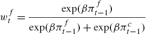
in which πf![]() and πc
and πc![]() are measures of fundamentalists' and chartists' performance, respectively.
are measures of fundamentalists' and chartists' performance, respectively.
In this setup, the coefficient β captures the switching behavior of agents, or their sensitivity to performance differences, and is typically denoted the intensity of choice parameter. With β=0![]() , agents are not sensitive to differences in performance between groups and remain within their group with probability 1. With β>0
, agents are not sensitive to differences in performance between groups and remain within their group with probability 1. With β>0![]() , agents are sensitive to performance differences. In the limit, as β tends to infinity, agents switch to the most profitable group with probability 1 such that wft∈{0,1}
, agents are sensitive to performance differences. In the limit, as β tends to infinity, agents switch to the most profitable group with probability 1 such that wft∈{0,1}![]() .
.
The significance of β in this configuration cannot be judged based on standard t-tests as it enters the expression non-linearly. Specifically, for β sufficiently large or sufficiently small, additional changes in β will not result in changes in wft![]() . As such, the standard errors of the estimated β will be inflated. To judge the significance of switching, one therefore needs to examine the model fit.
. As such, the standard errors of the estimated β will be inflated. To judge the significance of switching, one therefore needs to examine the model fit.
A second issue with this functional form is that the magnitude of β cannot be compared across markets or time periods. This is caused by the fact that its order of magnitude depends on the exact definition and the distributional characteristics of πft![]() . One way to address this issue, is to introduce normalized (unit-free) performance measures in a logit switching function, as first done in Ter Ellen and Zwinkels (2010):
. One way to address this issue, is to introduce normalized (unit-free) performance measures in a logit switching function, as first done in Ter Ellen and Zwinkels (2010):
(15) wft=11+exp(β(πct−1−πft−1πct−1+πft−1)).
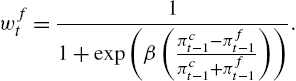
The additional benefit of this form is that the distribution of profit differences is less heavy-tailed, causing the estimation to be more precise and less sensitive to periods of high volatility.
Baur and Glover (2014) estimate a model for the gold market with chartists and fundamentalist who switch strategies according to their past performance. They find a significant improvement of fit against a benchmark model without such switching of strategies, but very different estimated parameters in different subsamples of the data. They also compare this analysis with switching depending on selected market statistics and find similar results for the parameters characterizing chartists' and fundamentalists' expectation formation under both scenarios.
3.4 Fundamental Value Estimate
Whereas the fundamentalist–chartist distinction in HAMs is intuitively appealing and consistent with empirical observation,7 the exact functional form of the two groups is less straightforward. Chartism is typically modeled using some form of expectation of auto-correlation in returns, which is consistent with the empirical results of Cutler et al. (1991), who find autocorrelation in the returns of a broad set of assets, and it is also consistent with the tendency of people to erroneously identify trends in random data.8 Fundamentalism is typically modeled as expected mean reversion towards the fundamental value. The main question is, though, what this fundamental value should be.
There are several theoretical properties any fundamental value should have. Therefore, in analytical or simulation settings it is possible to formulate a reasonable process for the fundamental value. Empirically though, one has to choose a specific model. Note, however, that the fundamental value used in an empirical HAM is not necessarily the actual fundamental value of the asset. HAMs are based on the notion of bounded rationality, and it is therefore internally consistent to also assume this for the ability of fundamentalists to calculate a fundamental value. As such, the choice of fundamental value should be based on the question whether a boundedly rational market participant could reasonably make the same choice. In other words, the fundamental value should also be a heuristic.
A number of studies using equity data, starting with Boswijk et al. (2007), use a simple fundamental value estimate based on the Gordon-growth model or dividend-discount model; see Gordon and Shapiro (1956). The model is given by
(16) P⁎t=1+gr−gyt
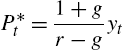
in which yt![]() is dividend, g is the constant growth rate of dividends, and r is the required return or discount factor.
is dividend, g is the constant growth rate of dividends, and r is the required return or discount factor.
The advantage of this approach is certainly its simplicity. The drawback is that it does not take time-variation of the discount factor into account, as is common in mainstream asset pricing studies, cf. Cochrane (2001). This causes the fundamental value estimate P⁎t![]() to be rather smooth because the discount factor is assumed constant. As such, models using this fundamental value estimate might attribute an excessive amount of price volatility to non-fundamental factors. Hommes and in 't Veld (2017) are the first to address this issue and introduce a stochastic discount factor in HAMs. Specifically, next to the typical Gordon growth model they create a fundamental value estimate based on the Campbell and Cochrane (1999) consumption-habit model. The latter constitutes a typical consumption-based asset pricing model and therefore belongs to a different class of asset pricing models than the endowment based HAMs. The authors find evidence of behavioral heterogeneity, regardless of the underlying fundamental value estimate. Whereas Hommes and in 't Veld (2017) do not fully integrate the two approaches, their paper constitutes an interesting first step towards integrating the two lines of research, which might also help in getting the heterogeneity approach more widely accepted in the mainstream finance and economics literature.9
to be rather smooth because the discount factor is assumed constant. As such, models using this fundamental value estimate might attribute an excessive amount of price volatility to non-fundamental factors. Hommes and in 't Veld (2017) are the first to address this issue and introduce a stochastic discount factor in HAMs. Specifically, next to the typical Gordon growth model they create a fundamental value estimate based on the Campbell and Cochrane (1999) consumption-habit model. The latter constitutes a typical consumption-based asset pricing model and therefore belongs to a different class of asset pricing models than the endowment based HAMs. The authors find evidence of behavioral heterogeneity, regardless of the underlying fundamental value estimate. Whereas Hommes and in 't Veld (2017) do not fully integrate the two approaches, their paper constitutes an interesting first step towards integrating the two lines of research, which might also help in getting the heterogeneity approach more widely accepted in the mainstream finance and economics literature.9
Studies focusing on foreign exchange markets typically use the Purchasing Power Parity (PPP) model as fundamental value estimate; see e.g. Manzan and Westerhoff (2007); Reitz et al. (2006); Goldbaum and Zwinkels (2014). Kouwenberg et al. (2017) illustrate the added value of switching using different fundamental value estimates in a forecasting exercise for foreign exchange rates.
Alternatively, a number of studies circumvent the issue of choosing a particular model to proxy for the fundamental value. In each case, this approach yields a parsimonious proxy for a fundamental value, but also alters the exact interpretation of fundamentalist behavior. Furthermore, the approach is typically quite specific to a certain (institutional) framework and thereby less general. For example, De Jong et al. (2010) make use of the institutional framework of the European Monetary System (EMS), and use the central parity in the target zone regime as the fundamental. Whereas this provides a very clear and visible target, the group of fundamentalists no longer expect mean reversion towards the economic fundamental but expect the current institutional framework to be maintained without adjustments to the central parity.
Ter Ellen and Zwinkels (2010) use a moving average of the price level as fundamental value estimate. Whereas this is again a very parsimonious approach, the nature of fundamentalists in such a setup moves towards chartism as all expectations are based on market information. More recently, Frijns and Zwinkels (2016a, 2016b) have taken advantage of the fact that assets trade on multiple markets in formulating a fundamental value. Specifically, they use cross-listed stocks and the spot and derivatives markets, respectively. This changes the exact interpretation of fundamentalists towards arbitrageurs, but retains the stabilizing character of this particular group of market participants relative to the destabilizing chartists.
As we will see in the next section, the necessity of specifying the time development of the underlying fundamental value only applies to reduced-form models. When using a more general approach, it often suffices to assume a general law of motion of the fundamental value (e.g., Brownian motion). Estimation would, then, allow to identify, for instance, the variance of the innovations of the fundamental value along with the parameters of the agent-based part of the overall model. If the pertinent methodology allows filtering to retrieve unobserved variables, this would also provide an estimated trajectory of the fundamental value as the residual obtained by filtering the empirical data (raw prices or returns) by the behavioral component implied by the ABM. Note that such an approach is very different from the a priori specification of a plausible fundamental dynamic process in the models reviewed above.
4 Estimation Methods
4.1 Maximum Likelihood
4.1.1 General Considerations
By the very nature of agent-based models, maximum likelihood (ML) estimation without any numerical approximation will rarely be possible. Such a completely standard approach will indeed only be possible if the ABM can be represented by a reduced-form equation or a system of equations (e.g., a VAR structure) for which a standard ML estimation approach is available. Examples of such models have been covered in the previous section. Any such statistically convenient framework will be based upon relatively strong assumptions on the behavior of the underlying pool of agents. For instance, in order to end up with a reduced form that is equivalent to a (linear) regime-switching model (e.g. Reitz and Westerhoff, 2003), one has to assume that (i) two different groups of agents with two different linear demand functions exist, (ii) all the agents of one group are characterized by the same elasticities, (iii) markets are always dominated by one of the groups, and (iv) there is a unique (Gaussian) noise factor in each of these regimes. Condition (i) might be relaxed by having a less stringent microstructure based on a market-maker; condition (iii) might be relaxed by allowing for smooth transition models in the statistical implementation of the switching of strategies of agents along some discrete choice formalization.
Still, to be able to derive some simple macroscopic structural form of the agents' aggregate behavior, the stochastic factors have to be conceived a-priori as an additive noise superimposed on the agents' interaction. If, in principle, the agents' behavior is conceived to be of a stochastic nature (reflecting the inability of any model to completely cover all their motivations and idiosyncratic determinants of their behavior), this amounts to evoking the law of large numbers and resorting to the deterministic limiting process for an infinite number of agents in the population.
Maintaining the randomness of individual decisions as via a discrete choice formalization with a finite population would render the noise component of the model much more complicated: The noise would now consist of the set of all the stochastic factors entering the decision of all the agents in the model, i.e. with N agents the model would contain N stochastic processes rather than a single one as in typical structural equations. It is worthwhile to note that for typical candidates of the stochastic utility term in discrete choice models, like the Gumbel distribution, theoretical aggregation results are not available. Aggregation of individual decisions might also be hampered by correlation of their choices if social interactions are an important factor in the agents' decision process.
4.1.2 Maximum Likelihood Based on Numerical Integration
Full maximum likelihood for models with dispersed activity of an ensemble of agents would, in principle, require availability of closed-form solutions for the transient density of the process. Due to the complexity of most ABMs, such information will hardly ever be available. However, certain systems allow at least numerical approximations of the transient density that can be used for evaluation of the likelihood function. Lux (2009a) applies such a numerical approach to estimate a simple model of opinion formation for survey data of a business climate index. The underlying model assumes that agents switch between a pessimistic and optimistic expectation for the prospects of their economy under the influence of the opinion of their peers as well as exogenous factors (information about macroeconomic variables). For this model of social interaction, the transient density of the average opinion can be approximated via the so-called Fokker–Planck or forward Kolmogorov equation. The latter cannot be solved in closed form. However, as it is a partial differential equation, many well-known methods exist to integrate it numerically. It thus becomes possible to use a numerical ML estimator. Application to a business climate index for the German economy shows strong evidence of social interaction (herding), a significant momentum effect besides the baseline interaction and very limited explanatory power of exogenous economic variables.
This framework can, in principle, be generalized to more complex models with more than one dynamic process. Lux (2012) applies this approach to bivariate and trivariate processes. Here the underlying data consists of two sentiment surveys for the German stock market, short-run and medium-run sentiment, and the price of the DAX. The model allows for two interlinked opinion formation processes plus the dynamics of the stock index that might be driven by sentiment along with fundamental factors. Combining pairs of these three processes or all three simultaneously, the transient dynamics can again be approximately described by a (bivariate or trivariate) Fokker–Planck equation. These partial differential equations can again be solved numerically, albeit with much higher computational demands than in the univariate case. As it turns out, social interaction is much more pronounced in short-run than medium-run sentiment. It also turns out that both sentiment measures have little interaction (although they are obtained from the same ensemble of participants). The price dynamics show a significant influence of short-run sentiment which, however, could not be exploited profitably for prediction of stock prices in an out-of-sample forecasting exercise.
4.1.3 Approximate Maximum Likelihood10
When full maximum likelihood is not possible, various approximate likelihood approaches might still be feasible. For example, Alfarano et al. (2005) apply maximum likelihood based upon the stationary distribution of a financial market model with social interaction. Results would be close to the exact likelihood case only if the process converges quickly to its stationary distribution. In a similar framework, Kukacka and Barunik (2017) use the non-parametric simulated maximum likelihood estimator of Kristensen and Shin (2012) which uses simulated conditional densities rather than the analytical expressions and is, in principle, universally applicable. They show via Monte Carlo simulations that this approach can reliably estimate the parameters of a strategy-switching model à la Brock and Hommes (1997). They find significant parameters of the expected sign for the fundamentalist and chartist trading strategies for various stock markets, but the ‘intensity of choice’ parameter turns out to be insignificant which is also found by a number of related studies on similar models.
4.2 Moment-Based Estimators
4.2.1 General Considerations
A most straightforward way to estimate complex models is the Generalized Method of Moments (GMM) and the Simulated Method of Moments (SMM) approach. The former estimates parameters by matching a weighted average of analytical moments, the later uses simulated moments in cases in which analytical moments are not available. Both GMM and SMM have a long legacy of applications in economics and finance (cf. Mátyás, 1999) and should be flexible enough to also be applicable to agent-based models. However, even this very general approach might have to cope with specific problems when applied to typical agent-based models. One of these is the lack of continuity of many moments when varying certain parameters. To see this, consider an ensemble of agents subject to a discrete choice problem of deciding about the most promising trading strategy at any time, where, for the sake of concreteness, we denote the alternatives again as ‘chartism’ and ‘fundamentalism’. There will be two probabilities pcf(⋅)![]() and pfc(⋅)
and pfc(⋅)![]() for switching from one alternative to the other, both depending on statistics of the current and past market development. A simple way to simulate such a framework consists of drawing uniform numbers εi
for switching from one alternative to the other, both depending on statistics of the current and past market development. A simple way to simulate such a framework consists of drawing uniform numbers εi![]() for each agent i and making this agent switch if εi<pcf(⋅)
for each agent i and making this agent switch if εi<pcf(⋅)![]() or pfc(⋅)
or pfc(⋅)![]() depending on which is applicable.
depending on which is applicable.
The important point here is that this type of stochasticity at the level of the individual agent is distinctly different from a standard additive noise at the system level. Even when fixing the sequence of random numbers, any statistics derived from this process will not be smooth under variation of the parameters of the model. Namely, if we vary any parameter that enters as a determinant of pcf(⋅)![]() or pfc(⋅)
or pfc(⋅)![]() and keep the set of random draws constant, there will be a discontinuous move at some point making the agent switch her behavior. The same, of course, applies to all other agents, so that in contrast to a deterministic process with linear noise, a stochastic process with noise at the level of the agent will exhibit in general non-smooth statistics even with “frozen” random draws.
and keep the set of random draws constant, there will be a discontinuous move at some point making the agent switch her behavior. The same, of course, applies to all other agents, so that in contrast to a deterministic process with linear noise, a stochastic process with noise at the level of the agent will exhibit in general non-smooth statistics even with “frozen” random draws.
Luckily, this does not necessarily make all standard estimation methods unfeasible. While standard regularity conditions will typically require smoothness of the objective functions, more general sets of conditions can be established that allow for non-smooth and non-differentiable objective functions, cf. Andrews (1993). The more practical problem is that the rugged surface resulting from such a microfounded process would render standard derivative-based optimization routines useless.
Many recent papers on estimation of ABMs in economics have used various methods to match a selection of empirical moments. This should not be too surprising as, particularly in financial economics, the most prominent aim of the development of ABMs has been the explanation of the so-called stylized facts of asset returns. A list of such stylized facts includes (i) absence of autocorrelations in the raw returns at high frequencies or martingale-like behavior, (ii) leptokurtosis of the unconditional distribution of returns, or fat tails, (iii) volatility clustering or long-term temporal dependence in squared or absolute returns (or other measures of volatility), (iv) positive correlation between trading volume and volatility, and (v) long-term temporal dependence in volume and related measures of trading activity.
All of these features can be readily characterized by statistical moments of the underlying data, and quantitative measures of ‘stylized facts’ (i) to (iii) are typically used as the moments one attempts to match in order to estimate the models' parameter. Both in GMM and SMM, parameter estimates are obtained as the arguments of an objective function that consists of weighted deviations between the empirical and model-generated moments. According to our knowledge, stylized facts (iv) and (v) have been used to compare the output of agent-based models to empirical data (e.g., LeBaron, 2001) but have not been exploited so far in full-fetched estimation as all available studies concentrate on univariate series of returns and neglect other market statistics such as volume. Indeed, it even appears unclear whether well-known models that are able to match (i) to (iii) are also capable to explain the long-lasting autocorrelation of volume and its cross-correlation with volatility.
Almost all of the available literature also uses a simulated method of moments approach as the underlying models appear too complex to derive analytical moment conditions. An exception is Ghonghadze and Lux (2016).
4.2.2 Moment-Based Estimation of Structural Models
Within structural equation models Franke (2009) and Franke and Westerhoff (2011, 2012, 2016) have applied SMM estimation to a variety of models and have also conducted goodness-of-fit comparisons across different specifications. All the models considered are formulated in discrete time.
Franke (2009) estimates a model proposed by Manzan and Westerhoff (2007), which combines a market maker dynamics for price adjustments with a standard demand function of fundamentalists and a second group of traders, denoted speculators, who react to stochastic news. The author uses a sample of moments of raw and absolute returns, i.e. their means, autocovariances over various lags, and log absolute returns exceeding a certain threshold as a measure related to the tail index. Since it was found that the correlations between the moment conditions were too noisy, only the diagonal entries of the inverse of the variance–covariance matrix of the moment conditions has been used as weight matrix. Although the usual goodness-of-fit test, the so-called J-test for equality of empirical and model-generated moments, could always reject the model as the true data generating process for a sample of stock indices and exchange rates, the fit of the selected moments was nevertheless considered satisfactory.
Shi and Zheng (2016) consider an interesting variation of the discrete choice framework for switching between a chartist and fundamentalist strategy in which fundamentalists receive heterogeneous news about the change of the fundamental value. A certain fraction of agents then chooses one or the other strategy comparing their pertinent expected profits. In the infinite population limit, analytical expressions can be obtained for the two fractions. The resulting price process is estimated via analytical moments (GMM) from which the usual parameters of the demand functions of both groups and the dispersion of fundamental news relative to the agents' prior can be obtained.
Franke and Westerhoff (2011) estimate what they call a ‘structural stochastic volatility model’. This is a model of chartist/fundamentalist dynamics in which both demand functions consist of a systematic deterministic part and a noise factor with different variances for both groups. With an additional switching mechanism between groups this leads to volatility clustering in returns because of the different levels of demand fluctuations brought about by dominance of one or the other group. In their SMM estimation the authors use a weighting matrix obtained from bootstrapping the variability of the empirical moments. Results were again somewhat mixed: While the model could well reproduce the selected moments, the authors found that for two out of six parameters it could not be rejected that they were equal to zero in the application of the model to the US dollar–Deutsche Mark exchange rate series. Note that this implies that certain parts of the model seem to be superfluous (in this case the entire chartist component) and that a more parsimonious specification would probably have to be preferred. In the application to the S&P 500 returns, all parameters were significant. The same applies under a slightly different estimation procedure (Franke and Westerhoff, 2016). In the later paper, the authors also assess the goodness-of-fit of the model via a Monte Carlo analysis (rather than the standard J-test based on asymptotic theory) and found that under this approach, the model could not be rejected.
Franke and Westerhoff (2012), finally, use the SMM approach to conduct a model contest between two alternative formalizations of the chartist/fundamentalist approach: one with switching between strategies based on transition probabilities (the approach of their related papers of 2011 and 2016), and one using a discrete choice framework for the choice of strategy in any period. Further variations are obtained by considering different determinants in these switching or choice probabilities: the development of agents' wealth, herding and the effect of misalignment of asset prices. As it turns out, the discrete choice model with herding component in the fitness function performs best in matching the selected moments of S&P 500 returns.
Somewhat similar in spirit are the recent papers by Grazzini and Richiardi (2015), Lamperti (2015), and Barde (2016). Grazzini and Richiardi use a simulated minimum distance estimator for an agent-based model of price discovery in double auctions. Lamberti (2015) proposes an information-theoretical distance measure. Barde (2016) adopts a similar measure to compare different types of agent-based models. He abstains, however, from direct estimation, but compares the models for a large set of parameter values using the concept of model confidence set (Hansen et al., 2011) to select those models (with pre-specified parameters) that cannot be outperformed by other alternatives at a certain confidence level. As it turns out, the above mentioned model of Franke and Westerhoff (2016) is the one most often represented in the confidence set followed by the model of Alfarano et al. (2008).
4.2.3 Moment-Based Estimation of Models with Explicit Agents
The later is a model that in its original format is not in reduced form but has an ensemble of agents that update their behavior in continuous time. While the agents' aggregate behavior is represented by a Langevin equation in Barde (2016) – and hence the model is transformed into a structural one – Jang (2015) studies simulated method of moments estimation for the same framework on the base of proper micro-simulations. He shows that the objective function is non-smooth (cf. the considerations laid out in Section 4.2.1) and also exhibits very flat areas along various dimensions which makes identification of a global minimum difficult. Jang explores the behavior of the SMM estimator in various ways fixing some parameters, and estimating the remaining ones. He finds certain intervals for some of the parameters in which Hansen's J-test does not reject the model as the ‘true’ data generating process.
When using a model based upon a proper micro-ensemble of agents, a particular conundrum is the decision about the number of agents. Replicating the market dynamics using the ‘true’ number of market participants appears out of the question. Since this number is probably in the millions for typical stock and foreign exchange markets of advanced economies, this would impose too high a computational burden on most models. In addition, exact numbers are often not known and might show some variation over time. What is more, practically all models available in the literature would become “uninteresting” with this large number of agents. The reason is that despite being subject to all types of social interaction agents are mostly autonomous in their decisions and with a given intensity of interaction the system will eventually tend to a limiting behavior under a law of large numbers when one increases the number of market participants. Typically the limiting behavior would lead to Gaussian market statistics lacking all the stylized facts of financial returns.
Since the stylized facts appear largely independent of the varying size of different markets, it appears appropriate to design behavioral agent-based models that show robust stylized facts independent of system size. Various avenues to arrive at models that maintain strong coherence of behavior also in large populations are laid out in Aoki (2002), Alfarano et al. (2008), Alfarano and Milakovic (2009), and Irle et al. (2011). Lux (2009a) estimates the system size (number of agents) for macroeconomic survey data of which the number of participants is known, and finds a much smaller (as he calls it) ‘effective’ system size that he attributes to agents moving in tandem with each other in certain groups. This resonates with the important observation emphasized by Chen (2002) that, in principle, the noise-over-signal ratio of some observable should provide an indication on how many independent contributing factors one should expect in a model explaining its behavior. Indeed, Jang (2015) considers different numbers of agents and finds a monotonic improvement of the goodness-of-fit when increasing the number of agents from 10 to 1000 in his estimation of the Alfarano et al. (2008) model for five foreign exchange rates. In his application, he also finds relatively uniform parameter estimates across markets (assuming N=100![]() ), and a contribution of about fifty percent of the agent-based speculative dynamics to the overall volatility of exchange rates.
), and a contribution of about fifty percent of the agent-based speculative dynamics to the overall volatility of exchange rates.
Ghonghadze and Lux (2016) and Chen and Lux (2016) both continue the line of research initiated by Jang (2015). Ghonghadze and Lux (2016) expand analytical results of Alfarano et al. (2008) to derive a generalized methods of moments estimator, while Chen and Lux use a similar set of moments in an SMM approach. Chen and Lux (2016) come to the conclusion that due to the lack of smoothness of the objective function, a one-time optimization from a given set of initial conditions could lead to almost arbitrary results. Hence, a more systematic exploration of the parameter space is needed. They recommend an extensive grid search followed by an application of a derivative-free optimization method for a range of the best grid values found in the first step. With GMM, more standard optimization routines can be applied, but nevertheless the parameters of the Alfarano et al. (2008) model appear difficult to estimate as there are strong correlations between certain parameters. The system appears near to collinearity and with not too large sample size (say some thousand observations as is typical in financial data) certain sets of parameter values could generate apparently very similar dynamics. Again, a grid search prior to the application of an optimization routine appears useful.
It is also found that very large samples are needed (about 105 observations) for SMM to approach the efficiency of GMM. While with sufficiently larger sample sizes, both GMM and SMM estimate the parameters more precisely and show a tendency towards T1/2![]() consistency, in both cases the J-test of goodness-of-fit based on the overidentification restrictions shows severe size distortion. In particular, while the asymptotic χ2
consistency, in both cases the J-test of goodness-of-fit based on the overidentification restrictions shows severe size distortion. In particular, while the asymptotic χ2![]() distribution fits the experimental distribution of the J-test well for a minimal set of moments, it tends to over-accept its null when additional moments are added in the estimation. This behavior stems very likely from the limited added informational content of further moment conditions. This might signal a general problem for GMM/SMM estimation of ABMs in the context of univariate financial data: there are not too many moments one can use in such exercises. Basically, all available studies use some measure of fat-tailedness and clustering of volatility. Adding more moments, one can just add alternative measures (like, e.g., autocovariances over different lags) that are highly correlated with each other.
distribution fits the experimental distribution of the J-test well for a minimal set of moments, it tends to over-accept its null when additional moments are added in the estimation. This behavior stems very likely from the limited added informational content of further moment conditions. This might signal a general problem for GMM/SMM estimation of ABMs in the context of univariate financial data: there are not too many moments one can use in such exercises. Basically, all available studies use some measure of fat-tailedness and clustering of volatility. Adding more moments, one can just add alternative measures (like, e.g., autocovariances over different lags) that are highly correlated with each other.
In the empirical part of their papers, both Chen and Lux (2016) and Ghonghadze and Lux (2016) apply their estimation algorithm to a selection of stock and foreign exchange data as well as the price of gold. Although the estimated parameters are not always very close, overall the results confirm received wisdom: Speculative forces appear stronger in stock markets and the market for gold than in foreign exchange markets. Ghonghadze and Lux (2016) also conduct a forecasting competition between their ABM and a standard GARCH model. While the GARCH has throughout somewhat smaller errors of its volatility forecasts, it turns out that the ABM can add value when combined forecasts from both models are constructed. It is also shown that for medium and long-run horizons (10 to 50 days forecasts) the GARCH model does not ‘encompass’ the ABM, i.e. the forecasts of the later uses information that is not already covered by the GARCH model (which motivates combining their forecasts).
4.3 Agent-Based Models as Latent Variable Models and Related Estimators
4.3.1 Basic Framework
It has been mentioned in Section 2 that agent-based models of ecological processes have often been framed as state-space or hidden Markov models, and have been estimated by a variety of methods developed for this class of models. Indeed, it appears to us that most models that have been reviewed above can be easily categorized as examples of state-space models or slightly more general latent variable models, so that estimation of ABMs could profit substantially from the rich toolbox developed for such models. As far as we can see, economic ABMs have never been related to the framework of state-space models, with the exception of a recent paper by Grazzini et al. (2017) who, however focus only on Bayesian estimation within such a context and do not emphasize the general proximity of ABMs to state-space models.
In other areas of economics, state-space modeling is more common: For instance, dynamic stochastic general equilibrium (DSGE) models have been estimated with both frequentist and Bayesian methods based upon a state-space representation, cf. Fernández-Villaverde and Rubio-Ramírez (2007), and Amisano and Tristani (2010) for both frequentist and Bayesian methods, as well as the monograph by Herbst and Schorfheide (2016) that focuses completely on Bayesian estimation which has become particularly popular in this area. In financial econometrics, similarly popular areas of applications are stochastic volatility models (e.g. Kim et al., 1998; Carvalho and Lopes, 2007) and Markov-switching models (e.g. Billio and Casarin, 2010). A survey of a range of popular approaches can be found in Lopes and Tsay (2011).
Since state-space modeling seems an important concept in which agent-based models could be nested as a particular subset of cases, we provide here a short introduction together with an illustrative application of important methods for parameter estimation to a prominent ABM. A general state-space model is defined by the stochastic evolution in time of a vector of states, say xt![]() , and a vector of measurements, say yt
, and a vector of measurements, say yt![]() . If xt
. If xt![]() follows a general Markov process, the unobserved process for the state vector can be written as
follows a general Markov process, the unobserved process for the state vector can be written as
(17) xt=f(xt−1,εt)
where εt![]() is a summary notation for all stochastic factors that enter into the dynamics of xt
is a summary notation for all stochastic factors that enter into the dynamics of xt![]() . The vector of observations can be written in a similar general form as
. The vector of observations can be written in a similar general form as
(18) yt=g(xt,ηt)
where ηt![]() summarizes all stochastic factors that make the vector of measurements a noisy signal of the states xt
summarizes all stochastic factors that make the vector of measurements a noisy signal of the states xt![]() . If Eqs. (17) and (18) are linear systems of equations with Gaussian noises, the optimal approach to parameter estimation and filtering for recovery of the unobserved state vector is the well-known Kalman filter. For nonlinear systems with Gaussian noises, various extensions and approximations to the linear Kalman filter have been developed (see e.g. Grewal and Andrews, 2008). For nonlinear, non-Gaussian state-space models, Markov chain Monte Carlo and particle filter methods have become the state of the art (cf. Doucet et al., 2001).
. If Eqs. (17) and (18) are linear systems of equations with Gaussian noises, the optimal approach to parameter estimation and filtering for recovery of the unobserved state vector is the well-known Kalman filter. For nonlinear systems with Gaussian noises, various extensions and approximations to the linear Kalman filter have been developed (see e.g. Grewal and Andrews, 2008). For nonlinear, non-Gaussian state-space models, Markov chain Monte Carlo and particle filter methods have become the state of the art (cf. Doucet et al., 2001).
Many agent-based models can be cast into the framework of Eqs. (17) and (18). Others can be embedded into slightly more general classes of models with latent variables. This basically applies to practically all the ABMs for interaction of heterogeneous investors that we have reviewed in the preceding sections. What distinguishes agent-based models from other state-space models is that Eq. (17) captures some sort of summary statistics of relevant features of the agents averaged over the entire ensemble of actors that is of relevance for the dynamics of the observables yt![]() , most often asset prices or returns. If the behavior of individual agents is formalized in a stochastic way (taking into account idiosyncratic factors unknown to the modeler), Eq. (17) would not only contain one noise factor for each element of the state vector, but would also be driven by the joint dynamics of agents' changes of behavior and their respective stochastic elements. While we could imagine a state-space formalism in which not a summary measure, but the exact features of each agent define the vector of states, such a model would presumably be hard or impossible to estimate just because a small number of observed variables would almost surely not contain enough information to track a much larger number of states.
, most often asset prices or returns. If the behavior of individual agents is formalized in a stochastic way (taking into account idiosyncratic factors unknown to the modeler), Eq. (17) would not only contain one noise factor for each element of the state vector, but would also be driven by the joint dynamics of agents' changes of behavior and their respective stochastic elements. While we could imagine a state-space formalism in which not a summary measure, but the exact features of each agent define the vector of states, such a model would presumably be hard or impossible to estimate just because a small number of observed variables would almost surely not contain enough information to track a much larger number of states.
4.3.2 Illustration: A Nonlinear Model of Speculative Dynamics with Two Groups of Agents
We take as an example a simple heterogeneous agent model with two types of traders that has been proposed by Gaunersdorfer and Hommes (2007). In this model, the two types are chartists and fundamentalists, and their demand functions, zc,t![]() and zf,t
and zf,t![]() are particular cases of Eq. (4) of the following form:
are particular cases of Eq. (4) of the following form:
(19) zc,t=Pt−1+g(Pt−1−Pt−2)+y−RPtaσ2zf,t=Pf+ν(Pt−1−Pf)+y−RPtaσ2
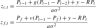
where y is the expected dividend (here assumed to be constant). Risk aversion a and expected variance of price changes, σ2![]() , are assumed to be the same for both groups, and R=1+r
, are assumed to be the same for both groups, and R=1+r![]() . Agents' choice of strategy is determined by a discrete-choice approach based upon accumulated profits:
. Agents' choice of strategy is determined by a discrete-choice approach based upon accumulated profits:
(20) Uh,t=(Pt+y−RPt−1)zh,t−1+ηUh,t−1
for h=c,t![]() , with η∈[0,1]
, with η∈[0,1]![]() a memory parameter for the influence of past profits. Gaunersdorfer and Hommes (2007) assume an infinite population so that the fractions nc,t
a memory parameter for the influence of past profits. Gaunersdorfer and Hommes (2007) assume an infinite population so that the fractions nc,t![]() and nf,t
and nf,t![]() of the two groups within the overall population would be identical to their expectations:
of the two groups within the overall population would be identical to their expectations:
(21) nh,t=exp(βUh,t−1)∑m=c,fexp(βUm,t−1)
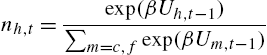
with β the parameter for the intensity of choice.
In addition, the authors assume that the fraction of chartists also decreases when the price deviates strongly from its fundamental value so that effectively, the two fractions are given by ˜nc,t![]() and ˜nf,t
and ˜nf,t![]() defined as follows:
defined as follows:
(22) ˜nc,t=nc,texp(−(Pt−1−Pf)2α),˜nf,t=1−˜nc,t,
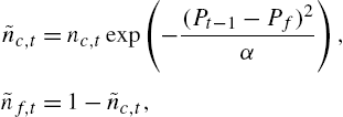
with α>0![]() , a constant parameter for the strength of the stabilizing force of the fundamental value. In the stochastic version of the model, a random Gaussian term ut∼N(0,σ2u)
, a constant parameter for the strength of the stabilizing force of the fundamental value. In the stochastic version of the model, a random Gaussian term ut∼N(0,σ2u)![]() is added to the system so that the asset price in a market equilibrium with zero exogenous supply is given by
is added to the system so that the asset price in a market equilibrium with zero exogenous supply is given by
(23) RPt=˜nc,tEc,t[Pt+1+y]+˜nf,tEf,t[Pt+1+y]+ut
with the expectations given by the first two terms in the numerators of the right-hand sides of Eqs. (19), i.e.
(24) Ec,t[Pt+1+y]=Pt−1+g(Pt−1−Pt−2)+y,Ef,t[Pt+1+y]=Pf+ν(Pt−1−Pf)+y.

Obviously, Eq. (23) is a well-defined equation for the observed variable – the asset price – of this dynamic system. Eqs. (19) through (22) constitute the state dynamics with ˜nc,t![]() , and ˜nf,t
, and ˜nf,t![]() being unobserved state variables, while Pt
being unobserved state variables, while Pt![]() is the observable part of the system. In the original model with its assumption of an infinite population this would be a completely deterministic system and, thus, would be a somewhat degenerate case of a state-space system. A case that is more representative of the ABM literature is easily obtained by rather assuming that the population of investors is finite and applying Eqs. (21) and (22) not as deterministic expressions, but to draw binomial random numbers with the pertinent probabilities to independently determine for each agent her choice of strategy at time t. This can simply be achieved by binomial draws with probabilities:
is the observable part of the system. In the original model with its assumption of an infinite population this would be a completely deterministic system and, thus, would be a somewhat degenerate case of a state-space system. A case that is more representative of the ABM literature is easily obtained by rather assuming that the population of investors is finite and applying Eqs. (21) and (22) not as deterministic expressions, but to draw binomial random numbers with the pertinent probabilities to independently determine for each agent her choice of strategy at time t. This can simply be achieved by binomial draws with probabilities:
(25) Pr(c)=exp(βUc,t−1)exp(βUc,t−1)+exp(βUf,t−1)exp(−(Pt−1−Pf)2α)andPr(f)=1−Pr(c)

with the obvious notation indicating the probability to select the chartist or fundamentalist strategy by Pr(c)![]() and Pr(f)
and Pr(f)![]() , respectively. The stochastic fractions of chartists and fundamentalists generated in this way replace the laws of Eqs. (22) and (23). Eqs. (20) and (25) would then constitute our implementation of the state dynamics which apparently is both highly nonlinear and non-Gaussian. Indeed, in this example the stochastic factors that are symbolized in Eq. (17) by the summary notation εt
, respectively. The stochastic fractions of chartists and fundamentalists generated in this way replace the laws of Eqs. (22) and (23). Eqs. (20) and (25) would then constitute our implementation of the state dynamics which apparently is both highly nonlinear and non-Gaussian. Indeed, in this example the stochastic factors that are symbolized in Eq. (17) by the summary notation εt![]() consist of as many stochastic draws as there are agents in the system. However, the state of the system can still be conveniently summarized by the (now stochastic) fractions of chartists and fundamentalists which enter again in the price dynamics as formalized in Eq. (23).
consist of as many stochastic draws as there are agents in the system. However, the state of the system can still be conveniently summarized by the (now stochastic) fractions of chartists and fundamentalists which enter again in the price dynamics as formalized in Eq. (23).
Note that our overall system is of a more general format than the state space formalism introduced in Eqs. (17) and (18). Namely, the unobserved state (here ˜nc,t![]() ) does not follow an autonomous Markov process but also depends on lagged values of the observation, Pt
) does not follow an autonomous Markov process but also depends on lagged values of the observation, Pt![]() . In the absence of stochastic factors in the state dynamics, such a process is often characterized as an ‘observation-driven process’ (cf. Douc et al., 2013). The more general case encountered here would fall under the label of a ‘dynamic system with latent variables’. An interesting example from empirical finance with a similar format is a stochastic volatility model with a leverage effect (leading to dependency of the latent volatility process on past realizations of returns, cf. Yu, 2005; Pitt et al., 2014).
. In the absence of stochastic factors in the state dynamics, such a process is often characterized as an ‘observation-driven process’ (cf. Douc et al., 2013). The more general case encountered here would fall under the label of a ‘dynamic system with latent variables’. An interesting example from empirical finance with a similar format is a stochastic volatility model with a leverage effect (leading to dependency of the latent volatility process on past realizations of returns, cf. Yu, 2005; Pitt et al., 2014).
The dynamics of the present system is well understood: In particular, for certain parameter values its deterministic ‘skeleton’ (with ut=0![]() ) is characterized by a locally stable fixed point (with the price equal to the fundamental value) and a limit cycle that also possesses its own domain of attraction. Adding noise of sufficient amplitude, the stochastic system switches repeatedly between these two attractors and the noisy cyclical episodes lead to returns that to some extent show leptokurtosis and volatility clustering (cf. also Lux and Alfarano, 2016). The lower left-hand panel of Fig. 1 exhibits a typical example of the state dynamics (fraction of chartists nc,t
) is characterized by a locally stable fixed point (with the price equal to the fundamental value) and a limit cycle that also possesses its own domain of attraction. Adding noise of sufficient amplitude, the stochastic system switches repeatedly between these two attractors and the noisy cyclical episodes lead to returns that to some extent show leptokurtosis and volatility clustering (cf. also Lux and Alfarano, 2016). The lower left-hand panel of Fig. 1 exhibits a typical example of the state dynamics (fraction of chartists nc,t![]() ): Mostly the market is dominated by fundamentalists (namely, when the process is close to the fixed point equilibrium), but rapid eruptions of periods with adaption of a chartist strategy by many market participants occur repeatedly (when the stochastic factor drives the dynamics into the domain of the limit cycle).
): Mostly the market is dominated by fundamentalists (namely, when the process is close to the fixed point equilibrium), but rapid eruptions of periods with adaption of a chartist strategy by many market participants occur repeatedly (when the stochastic factor drives the dynamics into the domain of the limit cycle).

When bringing such a model to data, one typically would pursue two objectives: (i) estimating the parameters, and (ii) tracking the unobserved state on the base of the observable variables. Moment-based methods (cf. Section 4.2) could be applied for parameter estimation, but they would not provide an avenue for filtering information on unobserved states. Indeed, despite the prominent role of summary variables for agents' states (strategies, expectations, opinions), hardly any attempts have been made in the ABM literature to retrieve information on such unobserved variables.
4.3.3 Estimation of the Model of Gaunersdorfer and Hommes Based on Particle Filter Algorithms
We will now shortly explain how to estimate the parameters and how to track the states of such a highly nonlinear system with dispersed activity via state-space methods. Like many agent-based models, the present framework also has probably too many free parameters, that could not all be estimated at the same time with the limited information available from the price dynamics. We will, therefore, concentrate on four crucial parameters: the reaction parameters of chartists and fundamentalists, g and ν, the intensity of choice, β, and the variance σ2u![]() of the noise component of the ‘measurement equation’ (23). Overall, we adopt the parameters of the simulations conducted by Gaunersdorfer and Hommes (2007): ν=1.0
of the noise component of the ‘measurement equation’ (23). Overall, we adopt the parameters of the simulations conducted by Gaunersdorfer and Hommes (2007): ν=1.0![]() , g=1.9
, g=1.9![]() , β=2.0
, β=2.0![]() , σu=10
, σu=10![]() , r=0.001
, r=0.001![]() , α=1800
, α=1800![]() , aσ2=1
, aσ2=1![]() , η=0.99
, η=0.99![]() , Pf=1000
, Pf=1000![]() , and y=1
, and y=1![]() .
.
We illustrate the design and performance of Monte Carlo methods developed for state-space models with three basic approaches: (i) frequentist maximum likelihood based on a particle filter, (ii) an evolutionary algorithm known as self-organizing state-space modeling, and (iii) Bayesian sequential Markov chain Monte Carlo. We dispense with many technical details which can be found in the vast statistical literature on this subject and its applications to DSGE models, ecological models as well as in financial econometrics.
Frequentist ML Estimation via a Particle Filter
Denote by θ={ν,g,β,σu}![]() the vector of parameters. The likelihood function with a sample of observations of asset prices Pt
the vector of parameters. The likelihood function with a sample of observations of asset prices Pt![]() , t=1,…,T
, t=1,…,T![]() is
is
(26) L(P1,…,PT|t)=p(P1|θ)T∏t=2p(Pt|Pt−1,θ)

in which in the absence of a closed-form solution for the unconditional density, the first term, p(P1|θ)![]() can be obtained from the simulated stationary distribution on the base of a sufficiently long Monte Carlo simulation of the model. The conditional densities p(Pt|Pt−1,θ)
can be obtained from the simulated stationary distribution on the base of a sufficiently long Monte Carlo simulation of the model. The conditional densities p(Pt|Pt−1,θ)![]() summarize the temporal evolution of the state-space model and can be decomposed as follows:
summarize the temporal evolution of the state-space model and can be decomposed as follows:
(27) p(Pt|Pt−1,θ)=∫p(Pt|nc,t)P(nc,t|nc,t−1)dnc,t−1
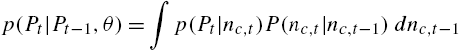
where we have summarized the state of the latent variables by nc,t![]() .
.
While the first conditional density in the integral can be evaluated analytically in our case (but this need not be so), the second one can only be approximated via simulations.11 This motivates what has become known as the particle filter, i.e. discrete approximation of the terms p(Pt|Pt−1,θ)![]() via a set of ‘particles’. The most common approach to particle filtering works as follows12:
via a set of ‘particles’. The most common approach to particle filtering works as follows12:
- (i) Initiate a ‘swarm’ of B particles n(j)c,1,j=1,…,B
 using random draws from the unconditional distribution p(nc,θ)
 . If this is not known, one might simulate the complete state-space system to obtain an approximation of its unconditional density,13
 - (ii) the densities p(P1|n(j)c,1,θ)
 are computed and the particles are resampled using weights p(P1|n(j)c,1)∑mp(P1|n(m)c,1)
 ,
, - (iii) the resampled swarm is propagated through the state dynamics and the updated states n(j)c,2
 are obtained,
 - (iv) steps (ii) and (iii) are repeated for t=2,…,T
 .
.
In this way, we obtain an approximation of the likelihood function
(28) L(P1,…,PT|θ)≈T∏t=11NB∑j=1p(Pt|n(j)c,t,θ).
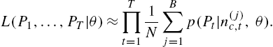
Under mild regularity conditions, the particle filter is a consistent estimator of the ‘true’ likelihood (e.g. Künsch, 2005) for baseline state space models. Ionides et al. (2011) show that for general systems with latent variables, an iterated filtering procedure on the base of a particle filter converges to the maximum likelihood estimate when the number of particles goes to infinity. Indeed, our example falls into this general class of models since there is a feedback from the observable variable Pt![]() to the unobservable state nc,t
to the unobservable state nc,t![]() which is absent in the elementary state-space formalism of Eqs. (17) and (18). One important problem is that the resulting approximation of the likelihood function is not a smooth function of the parameters. This is so because the multinomial draws in the resampling step would lead to discrete changes under continuous variation of the parameters of the model. This happens even if the random numbers are kept constant for subsequent iterations in the optimization routine (which one should nevertheless do in order not to introduce additional sources of discontinuities in the likelihood function).14
which is absent in the elementary state-space formalism of Eqs. (17) and (18). One important problem is that the resulting approximation of the likelihood function is not a smooth function of the parameters. This is so because the multinomial draws in the resampling step would lead to discrete changes under continuous variation of the parameters of the model. This happens even if the random numbers are kept constant for subsequent iterations in the optimization routine (which one should nevertheless do in order not to introduce additional sources of discontinuities in the likelihood function).14
Malik and Pitt (2011) have developed a method to make the approximation smooth via a simple transformation but very likely their approach will not provide a full remedy for this problem in an agent-based framework like ours since multinomial draws do not occur only in the resampling step of the particle filter (which Malik and Pitt's method smoothes out) but in the state dynamics as well. We will, therefore, generically have to use optimization algorithms that do not need derivatives as an input. Fernández-Villaverde and Rubio-Ramirez (2007) use simulated annealing to find the maximum of the likelihood function. Here, we resort to the versatile Nelder–Mead or simplex algorithm. Table 1 shows the results of a small Monte Carlo study using this particle filter approximation to the likelihood with simulated time series of length T=1000![]() and T=2000
and T=2000![]() (used as pseudo-empirical series) and also B=1000
(used as pseudo-empirical series) and also B=1000![]() and B=2000
and B=2000![]() particles.
particles.
Table 1
Monte Carlo experiment for estimation of Gaunersdorfer/Hommes model via Maximum Likelihood based on the particle filter
| Parameter | ν | g | β | σ u |
|---|---|---|---|---|
| True | 1.0 | 1.9 | 2.0 | 10.0 |
| T=1000 |
||||
| Mean | 0.999 | 1.585 | 2.235 | 10.048 |
| FSSE | 0.002 | 0.642 | 0.877 | 0.265 |
| RMSE | 0.003 | 0.712 | 0.904 | 0.268 |
|
B=2000
|
||||
| Mean | 0.999 | 1.617 | 2.186 | 10.058 |
| FSSE | 0.002 | 0.525 | 0.846 | 0.278 |
| RMSE | 0.003 | 0.594 | 0.862 | 0.282 |
| T=2000 |
||||
| Mean | 0.999 | 1.629 | 2.271 | 10.085 |
| FSSE | 0.001 | 0.452 | 0.666 | 0.202 |
| RMSE | 0.001 | 0.525 | 0.715 | 0.218 |
|
B=2000
|
||||
| Mean | 0.999 | 1.619 | 2.240 | 10.085 |
| FSSE | 0.001 | 0.493 | 0.714 | 0.214 |
| RMSE | 0.001 | 0.565 | 0.749 | 0.229 |

Notes: The table shows the means, finite sample standard errors (FSSE) and root-mean squared errors (RMSE) of 100 replications of each scenario.
As we can observe, in this example we get extremely accurate estimates of the parameter ν, reasonable estimates of σu![]() , and not very precise estimates of the remaining parameters g and β. We also see an improvement of the precision of our estimates when increasing the length of the underlying time series from T=1000
, and not very precise estimates of the remaining parameters g and β. We also see an improvement of the precision of our estimates when increasing the length of the underlying time series from T=1000![]() to T=2000
to T=2000![]() . The improvement is, however, smaller than expected under √T
. The improvement is, however, smaller than expected under √T![]() consistency. The reason is that we have used the same number of particles B. Since the overall approximation error increases with the length of a series, the approximation of the likelihood function requires an increase of the number of particles to off-set this tendency. Theoretical results on how B shall vary with T for convenient asymptotic behavior can be found in the statistical literature.15 As we can also observe in Table 1, increasing the number of particles for a constant length of the time series leaves the results basically unchanged. While this result can certainly not be generalized, it indicates that for the present sample sizes, more particles do not lead to a further gain in accuracy of the approximation. Estimated parameters could be used to filter out information on the unobservable state, and the outcome typically appears quite accurate in our application along the lines of the example displayed in the lower left-hand panel of Fig. 1.
consistency. The reason is that we have used the same number of particles B. Since the overall approximation error increases with the length of a series, the approximation of the likelihood function requires an increase of the number of particles to off-set this tendency. Theoretical results on how B shall vary with T for convenient asymptotic behavior can be found in the statistical literature.15 As we can also observe in Table 1, increasing the number of particles for a constant length of the time series leaves the results basically unchanged. While this result can certainly not be generalized, it indicates that for the present sample sizes, more particles do not lead to a further gain in accuracy of the approximation. Estimated parameters could be used to filter out information on the unobservable state, and the outcome typically appears quite accurate in our application along the lines of the example displayed in the lower left-hand panel of Fig. 1.
Estimation via Self-Organizing State Space Algorithm
A relatively simple alternative avenue to parameter estimation has been proposed by Kitagawa (1998) under this heading. The idea of this approach is to augment the state space by auxiliary particles. These auxiliary particles cover the unknown parameters. Hence, each particle in our setting would become a vector {n(j)c,t,ν(j)t,g(j)t,β(j)t,σ(j)u,t}![]() . The state dynamics would be augmented by trivial components:
. The state dynamics would be augmented by trivial components:
v(j)t+1=v(j)t,g(j)t+1=g(j)t,β(j)t+1=β(j)t,σ(j)u,t+1=σ(j)u,t
for j=1,…,B![]() the augmented particles.
the augmented particles.
The evaluation of the conditional densities in the likelihood function would, then, also exert evolutionary pressure on the auxiliary particles and lead to a selection of those that provide the highest conditional probabilities. By its construction, this approach is executed in one single sweep through the data. An example is shown in Fig. 1. The temporal evolution of the parameters is shown in terms of the mean over all particles for three of the parameters. While the overall length of the time series is T=1000![]() only the first 350 periods are displayed because the auxiliary parameters have completely converged at this stage, i.e. the shown mean is, in fact, the only value that has survived to this point and can, thus, count as the final estimate.
only the first 350 periods are displayed because the auxiliary parameters have completely converged at this stage, i.e. the shown mean is, in fact, the only value that has survived to this point and can, thus, count as the final estimate.
In this example, the estimation works satisfactorily: the final parameter estimates are close to their ‘true’ values. Particularly parameter ν is almost exactly identified after just a dozen of observations. Table 2 exhibits the statistics of a set of 100 Monte Carlo replications of the online estimation approach of which Fig. 1 has illustrated one single run. As the table shows overall results with T=1000![]() and B=1000
and B=1000![]() are somewhat worse in terms of root-mean squared errors (RMSEs) than with the ML approach. The advantage of this approach is an enormous saving in computation time: We only do one sweep through the data (i.e., estimate on-line) while the Nelder–Mead approach usually needed several hundreds of evaluations of the likelihood function over the whole length of the time series. We can, thus, easily increase the number of the particles. Table 2 also shows that the improvement when moving from B=1000
are somewhat worse in terms of root-mean squared errors (RMSEs) than with the ML approach. The advantage of this approach is an enormous saving in computation time: We only do one sweep through the data (i.e., estimate on-line) while the Nelder–Mead approach usually needed several hundreds of evaluations of the likelihood function over the whole length of the time series. We can, thus, easily increase the number of the particles. Table 2 also shows that the improvement when moving from B=1000![]() to B=10,000
to B=10,000![]() is, however, not too high and still inferior to the ML results. But one could certainly still increase B at reasonable costs.
is, however, not too high and still inferior to the ML results. But one could certainly still increase B at reasonable costs.
Table 2
Monte Carlo experiment for estimation of Gaunersdorfer/Hommes model via the Self-Organizing State Space Approach
| Parameter | ν | g | β | σ u |
|---|---|---|---|---|
| True | 1.0 | 1.9 | 2.0 | 10.0 |
| T=1000 |
||||
| Mean | 0.988 | 1.884 | 1.987 | 11.866 |
| FSSE | 0.044 | 0.820 | 1.094 | 2.470 |
| RMSE | 0.045 | 0.816 | 1.089 | 3.086 |
| T=1000 |
||||
| Mean | 0.994 | 1.716 | 2.071 | 10.944 |
| FSSE | 0.018 | 0.709 | 1.108 | 1.592 |
| RMSE | 0.018 | 0.729 | 1.105 | 1.844 |
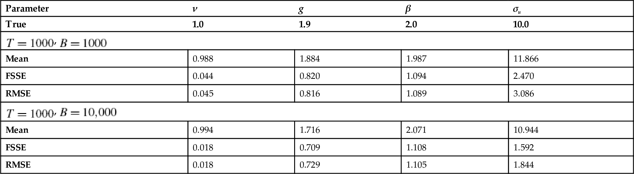
Notes: The table shows the means, finite sample standard errors (FSSE) and root-mean squared errors (RMSE) of 100 replications of each scenario.
One feature of this approach is that a larger time series of observations would not necessarily be of any benefit. With B=1000![]() particles, the distribution of the auxiliary particles has in almost all cases long become degenerate at the end of a time series of 1000 observations. Hence, no different estimates would be obtained with any longer series. With higher B, the swarm would likely remain heterogeneous for longer time, so that more efficient estimates would require an increase of both T and B at the same time. Despite these limitations, it is also worthwhile to emphasize the good performance of the filter for the state nc,t
particles, the distribution of the auxiliary particles has in almost all cases long become degenerate at the end of a time series of 1000 observations. Hence, no different estimates would be obtained with any longer series. With higher B, the swarm would likely remain heterogeneous for longer time, so that more efficient estimates would require an increase of both T and B at the same time. Despite these limitations, it is also worthwhile to emphasize the good performance of the filter for the state nc,t![]() . Note that the tracking of the state in this case is obtained on-line, i.e. with moving parameters as shown in the three remaining panels (plus the moving σu
. Note that the tracking of the state in this case is obtained on-line, i.e. with moving parameters as shown in the three remaining panels (plus the moving σu![]() that is not displayed here). Online estimation or particle learning is an active area of research, cf. Carvalho et al. (2010) and Ionides et al. (2011) for examples of more advanced approaches.
that is not displayed here). Online estimation or particle learning is an active area of research, cf. Carvalho et al. (2010) and Ionides et al. (2011) for examples of more advanced approaches.
Bayesian Estimation
We finally turn to Bayesian estimation, which is strongly connected with state-space approaches in the DSGE community. Andrieu et al. (2010) propose an approach that combines a particle filter with a Metropolis–Hastings sample of the posterior density of the parameters. This and closely related methods have been used by Fernández-Villaverde and Rubio-Ramirez (2007) for DSGE models and Golightly and Wilkinson (2011) for ecological agent-based models. The time-honored Metropolis–Hastings algorithm provides an approach to construct a Markov chain that converges to a stationary distribution equal to the posterior distribution of the parameter one wants to estimate. In order to generate this Markov chain, one needs a proposal density for new draws, say g(θζ|θζ−1)![]() where ζ is the sequential order of the chain. Draws from g(θζ|θζ−1)
where ζ is the sequential order of the chain. Draws from g(θζ|θζ−1)![]() , say θ⁎
, say θ⁎![]() , are accepted with probability
, are accepted with probability
α(θ⁎|θζ−1)=pθ⁎(y)p(θ⁎)g(θζ−1|θ⁎)pθζ−1(y)p(θζ−1)g(θ⁎|θζ−1)
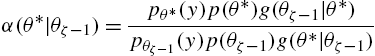
where pθ(y)![]() is the marginal likelihood of the observed data under θ, p(θ)
is the marginal likelihood of the observed data under θ, p(θ)![]() is the prior of the parameters, and the acceptance rate is restricted to the interval [0,1
is the prior of the parameters, and the acceptance rate is restricted to the interval [0,1![]() ] by appropriate constraints. In case the new draw θ⁎
] by appropriate constraints. In case the new draw θ⁎![]() is not accepted, the chain will continue with the previous values, i.e. θζ=θζ−1
is not accepted, the chain will continue with the previous values, i.e. θζ=θζ−1![]() . Under mild conditions on the likelihood of the process and the proposal density, the chain generated in this way will converge to the posterior distribution of the parameters. Andrieu et al. (2010) show that this convergence property holds also if the marginal likelihood is estimated via the particle filter introduced above. The pertinent method is called Particle Filter Markov Chain Monte Carlo (PMCMC). An important difference to the frequentist estimation presented earlier in this section is, however, that one would not initiate the particle filter with the same random seed in each iteration in order to generate random draws of the relative likelihoods.
. Under mild conditions on the likelihood of the process and the proposal density, the chain generated in this way will converge to the posterior distribution of the parameters. Andrieu et al. (2010) show that this convergence property holds also if the marginal likelihood is estimated via the particle filter introduced above. The pertinent method is called Particle Filter Markov Chain Monte Carlo (PMCMC). An important difference to the frequentist estimation presented earlier in this section is, however, that one would not initiate the particle filter with the same random seed in each iteration in order to generate random draws of the relative likelihoods.
We illustrate the Bayesian approach in Fig. 2 and Table 3. Since we might not have any clue to what the values of the parameters be prior to estimation, we used uniform priors with support in the interval [0,5![]() ] for ν,g
] for ν,g![]() and β and a uniform distribution on [0,50
and β and a uniform distribution on [0,50![]() ] for σu
] for σu![]() . For the proposal densities, we used random walks with standard deviations equal to 0.25 for the first three variables and 2.5 for the fourth. The underlying time series had a length of T=1000
. For the proposal densities, we used random walks with standard deviations equal to 0.25 for the first three variables and 2.5 for the fourth. The underlying time series had a length of T=1000![]() and we ran the algorithm with B=100
and we ran the algorithm with B=100![]() and B=1000
and B=1000![]() particles. The posterior distribution was sampled for a Markov chain of a length of 20,000 iterations after discarding the first 2000 iterations as transients.
particles. The posterior distribution was sampled for a Markov chain of a length of 20,000 iterations after discarding the first 2000 iterations as transients.

Table 3
Bayesian estimation of Gaunersdorfer/Hommes model via Particle Filter Markov Chain Monte Carlo
| T = 1000 |
B=100
|
B = 1000 | |||
|---|---|---|---|---|---|
| Parameter | True | Mean | S.E. | Mean | S.E. |
| ν | 1.0 | 0.999 | 0.008 | 0.999 | 0.006 |
| g | 1.9 | 1.938 | 0.124 | 1.968 | 0.116 |
| β | 2.0 | 3.139 | 1.340 | 2.610 | 1.362 |
| σ u | 10.0 | 10.396 | 0.715 | 10.184 | 0.349 |
| LogL | −3754.714 | 126.023 | −3735.381 | 110.455 | |
| Accept. rate | 0.352 | 0.375 | |||
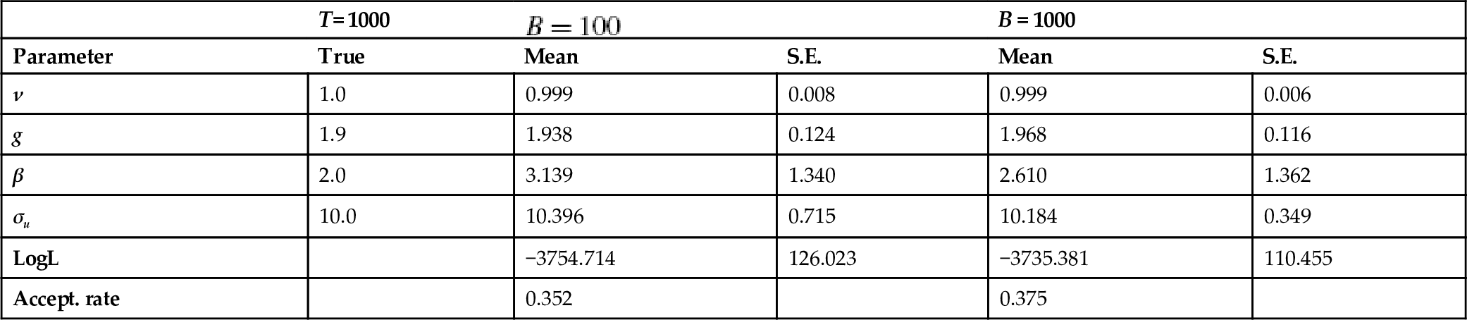
Notes: The table shows the Monte Carlo means and standard errors of the posterior distribution of the parameters from simulations with B=100![]() and B=1000
and B=1000![]() particles. The underlying time series has a length of T=1000
particles. The underlying time series has a length of T=1000![]() while the PMCMC algorithm used 20,000 iterations after discarding a transient of 2000 draws. Fig. 2 contains the transient indicating that convergence to the stationary posterior distribution is very fast.
while the PMCMC algorithm used 20,000 iterations after discarding a transient of 2000 draws. Fig. 2 contains the transient indicating that convergence to the stationary posterior distribution is very fast.
Fig. 2 shows the complete record or 22,000 iterations including the transients for B=100![]() . As we can see, we can hardly recognize any transient part at all: the Markov chain seems to converge to its stationary distribution very quickly. While this represents an estimation for only one replication of our ABM and the standard errors of the posterior distribution are not directly comparable to the finite sample standard errors across 100 simulations with the frequentist approach, results are pretty much in line with our previous findings. We see that the parameter ν seems to be almost perfectly identified even with as few as 100 particles followed by σu
. As we can see, we can hardly recognize any transient part at all: the Markov chain seems to converge to its stationary distribution very quickly. While this represents an estimation for only one replication of our ABM and the standard errors of the posterior distribution are not directly comparable to the finite sample standard errors across 100 simulations with the frequentist approach, results are pretty much in line with our previous findings. We see that the parameter ν seems to be almost perfectly identified even with as few as 100 particles followed by σu![]() and g with somewhat smaller signal-to-noise ratios. At least in our present example, the mean of the posterior distribution of g is remarkably close to the ‘true’ value and the signal-to-noise ratio of this parameter is relatively high so as to allow also meaningful inference on this parameter.
and g with somewhat smaller signal-to-noise ratios. At least in our present example, the mean of the posterior distribution of g is remarkably close to the ‘true’ value and the signal-to-noise ratio of this parameter is relatively high so as to allow also meaningful inference on this parameter.
This is, however, not the case with β, which eventually wanders across its entire admissible range (that we have fixed to the interval [0,5![]() ] via the choice of its prior). The mean and standard errors of β are so close to those of random draws from such a uniform distribution (2.5 and 1.445) that they appear meaningless, i.e. the data does not provide any information on β beyond that imposed by the distribution of the prior. Still, β>0
] via the choice of its prior). The mean and standard errors of β are so close to those of random draws from such a uniform distribution (2.5 and 1.445) that they appear meaningless, i.e. the data does not provide any information on β beyond that imposed by the distribution of the prior. Still, β>0![]() would be required for the scenario of long periods of fundamentalist dominance with recurrent bursts of chartist activity to be possible at all. The apparent inability to obtain sensible estimates of β resonates with empirical studies (using other methods) that always found it hard to obtain significant estimates of this parameter (see Boswijk et al., 2007; Kukacka and Barunik, 2017).
would be required for the scenario of long periods of fundamentalist dominance with recurrent bursts of chartist activity to be possible at all. The apparent inability to obtain sensible estimates of β resonates with empirical studies (using other methods) that always found it hard to obtain significant estimates of this parameter (see Boswijk et al., 2007; Kukacka and Barunik, 2017).
We note that for the Metropolis–Hastings algorithm the details of implementation are of secondary importance, as the theoretical convergence result holds under very general conditions. One major practical concern is the mixing of the Markov chain. A standard recommendation is an acceptance rate of 0.4, which both of our settings with B=100![]() and B=1000
and B=1000![]() get close to. With less mixing, a longer transient would be expected and the chain would have to be simulated over more iterations to obtain a satisfactory representation of the posterior density. The effect of a higher number of particles is a better approximation of the marginal likelihood which should also increase the precision of the estimation of the posterior distribution. This is indeed found to different degrees for the parameter ν, g and σu
get close to. With less mixing, a longer transient would be expected and the chain would have to be simulated over more iterations to obtain a satisfactory representation of the posterior density. The effect of a higher number of particles is a better approximation of the marginal likelihood which should also increase the precision of the estimation of the posterior distribution. This is indeed found to different degrees for the parameter ν, g and σu![]() , but not for β underlining the principal problem in estimating this parameter.
, but not for β underlining the principal problem in estimating this parameter.
Summarizing our findings in this subsection, we believe that the preceding experiments have demonstrated the great potential of sequential Monte Carlo methods for estimation of agent-based models. Adopting the rich toolbox available in this area would bring agent-based models to the same level of statistical rigor and precision as modern macroeconomics. What is more, in contrast to the hitherto popular moment-based estimators, SMC methods do not only allow inference on model parameters, but also filtering of information on unobserved state variables that characterize the agents' beliefs, opinions or attitudes. In the above example, we have also found that different parameters are estimated with very different degrees of precision. In particular, we found that the intensity of choice is almost impossible to estimate which also is in conformity with results obtained by other authors with other methods of inference. How general this phenomenon is and how much it impedes successful validation of agent-based models remains to be seen.
We also note that the Monte Carlo exercises above have been conducted on the base of a model formulated for prices as state variables, not returns. The lack of realism of some of the underlying assumptions such as the assumed dividend process would make an empirical implementation cumbersome. In Lux (2017), the same set of methods is applied to alternative asset pricing models with interacting agents that do not require any assumption on the dividend process. Monte Carlo exercises show very similar tendencies as in the present case, and the models under study are estimated for a selection of financial time series including a comparison of goodness-of-fit.
5 Applications of Agent-Based Models
Whereas the chapter has so far mainly focused on methods, we will now briefly turn to a description of the applications and results. As indicated before, the comparability of results across studies is rather limited due to the wide variation in both models and methods. It is therefore hard to make general statements about the behavior of agents across markets, or about which model is ‘best’. We will, however, provide an overview of what has been found so far using which type of data. We will divide the evidence in three levels: micro (individuals), market, and macro. The micro-level evidence focuses on the questions whether individuals form expectations as typically modeled in ABMs. It therefore serves as a check on the assumptions behind the models. The market level studies focus on one asset each, whereas the macro-level part focuses on general equilibrium models.
5.1 Micro-Level Applications
Because ABM and HAMs step away from the notion of rationality, they introduce a large number of degrees of freedom as there are many ways in which agents can behave boundedly rationally. As such, empirical research into the assumptions on expectation formation in ABMs is crucial. One challenge with micro-level studies is data availability. Whereas market outcomes (i.e., prices, volumes, etc.) are readily observable, market inputs at the individual level are mostly not observable. Therefore, one needs to turn to other sources of data than the standard macroeconomic and finance data bases. Several types of data for individual agents have been used, such as experimental data, survey data, and investment fund data, each with their own advantages and disadvantages. Whereas one can deduct revealed beliefs from experimental data, it is not clear to what extent experimental environments as well as their participants are representative for the real-life setting. Arifovic and Duffy (2018) give an overview of experimental work on ABMs. Survey data, on the other hand, is typically gathered among actual market participants based on actual markets. Unfortunately, it is unknown to the researcher, however, whether or not survey participants state their actual beliefs. This issue is partly mitigated when using publicly available survey data because the survey participant's reputation is at stake. Fund data, finally, consists of actual positions and capital flows, as certain types of funds are by law obliged to provide this information. The question that arises, though, is whether or not the observed actions are driven by beliefs, preferences, or institutional reasons. In what follows, we will give a sample of the empirical evidence from each of these data sources.
Both quantitative and qualitative surveys have been used for research in this area. Taylor and Allen (1992) show, based on a questionnaire survey, that 90% of the foreign exchange dealers based in London use some form of technical analysis in forming expectations about future exchange rates, particularly for short-term horizons. Menkhoff (2010) gathered similar data from fund managers in five different countries, and finds that 87% of the fund managers they survey are using technical analysis. Frankel and Froot (1986, 1990) were among the first to show, based on quantitative survey data, that expectations of market participants are non-rational and heterogeneous. They also find evidence for the chartist–fundamentalist approach employed in many of the heterogeneous agent models. Dick and Menkhoff (2013) use forecasters' self-assessment to classify themselves as chartists, fundamentalists, or a mix. They find that forecasters who characterize their forecasting tools as chartist use trend-following strategies and those that are categorized as fundamentalist have a stronger tendency toward purchasing power parity. For a more extensive overview, see Jongen et al. (2008).
Ter Ellen et al. (2013) are among the first to estimate a dynamic heterogeneous agent model on foreign exchange survey data. They find evidence for three forecasting rules (PPP, momentum, and interest parity) and that investors switch between forecasting rules depending on the past performance of these rules. Goldbaum and Zwinkels (2014) find that a model with fundamentalists and chartists can explain the survey data well. As in Ter Ellen et al. (2013), they find that fundamentalists are mean reverting and that this model is increasingly used for longer horizons. Chartists have contrarian expectations at the 1-month horizon. A model with time-varying weights obtained through an endogenous classification algorithm provides a substantially better fit than a static version of this model. Jongen et al. (2012) also allow the weights on different strategies to vary depending on market circumstances. However, instead of directly explaining the survey expectations, they analyze the dispersion between forecasts. They find that the dispersion is caused by investors using heterogeneous forecasting rules and having private information. This is in line with the earlier findings of Menkhoff et al. (2009) for a dataset on German financial market professionals.
The final data source we discuss here, is fund data. Given that both fund holdings and returns on the one hand and fund flows on the other hand are available, fund data allows us to study the behavior of both mutual fund investors as well as mutual fund managers. Goldbaum and Mizrach (2008) study the behavior of mutual fund investors and are able to estimate an intensity of choice parameter that governs to what extent investors switch between different types of mutual funds. They find that investors switch their allocation of capital between funds of similar styles but with different performance. A few more papers looks into the switching behavior of fund managers. Specifically, the question is to what extent fund managers switch between different styles presumably to maximize the performance of the fund. Using fund return data, the studies test whether the exposure to different styles is time-varying, and whether this time-variation is driven by relative past returns of the styles; see Verschoor and Zwinkels (2013) for foreign exchange funds, Schauten et al. (2015) for hedge funds, and Frijns et al. (2013) and Frijns and Zwinkels (2016a, 2016b) for mutual funds. Interestingly, the latter study finds that although fund managers massively switch capital towards styles that performed well in the recent past, this does not improve the overall performance of the fund nor does it attract more capital inflow. This is an indication that heterogeneity is indeed a behavioral characteristic.
5.2 Market-Level Applications
Due to the self-referential character of asset markets in ABMs, the behavioral heterogeneity of agents at the micro-level should be reflected in realized prices and returns. If a market is dominated by a particular type of agent, market dynamics should be more similar to the specific expectation formation model of that particular agent. As such, empirical evidence supporting the ABM approach can be identified from market data. A broad range of asset classes has by now been studied. Most papers so far have focused on equity markets. Boswijk et al. (2007) are among the first to estimate a HAM on market data. Specifically, they use historical data of the S&P 500 index and find significant evidence for behavioral heterogeneity at the annual frequency. Lof (2015) is based on the same dataset. Chiarella et al. (2012, 2014) and Amilon (2008) follow suit, on the monthly, weekly, and daily frequency, respectively. De Jong et al. (2009) study the Thai and Hong Kong stock markets simultaneously and find evidence for three types of agents, fundamentalists, chartists, and internationalists. Alfarano et al. (2007) use Japanese stock market data and find evidence for domination of noise traders. All these papers find evidence supportive of the heterogeneity approach in their respective models. Another common finding is that the intensity of choice or switching parameter is not significant based on common measures (i.e., a t-statistic). This finding could imply two things: Either there is no significant switching, or the intensity of choice is rather large such that the standard errors are inflated. Goodness of fit tests tend to suggest that adding switching increases the fit of the models, especially when the heterogeneous groups are well identified (i.e., when the fundamentalist and chartist coefficients are highly significant).
Rather than focusing on the return process of equity markets, a number of authors has employed an ABM to explain the volatility process of equity markets. Franke and Westerhoff (2012, 2016) develop and estimate a stochastic volatility model based on the premise that the stochastic noise terms of fundamentalist and chartist demand are different. By having time-varying weights on the different groups, this creates volatility clustering. Frijns et al. (2013) develop a model in which agents have different beliefs about the volatility process, which converges to a GARCH model with time-varying coefficients in which the ARCH-term and GARCH-term have conditional impacts. Ghonghadze and Lux (2016) apply GMM to the model of Alfarano et al. (2008) and show that the volatility forecasts of the HAM adds value to GARCH forecasts as it is not encompassed by the latter for certain assets and forecasting horizons. A typical finding in the volatility literature is that it is relatively straightforward to outperform a standard GARCH model in-sample, but much harder to do so out-of-sample. The volatility forecasting results based on ABMs are therefore encouraging.
Explaining foreign exchange market dynamics has long been an important motivation for the early HAM literature, which is also reflected in the amount of empirical work on this asset class; see Vigfusson (1997), Gilli and Winker (2003), Reitz and Westerhoff (2003), Ahrens and Reitz (2005), Reitz et al. (2006), Manzan and Westerhoff (2007), De Jong et al. (2010), Kouwenberg et al. (2017). The issue with such extremely liquid financial markets, though, is to find expectation formation rules that hold empirically as it is hard to find empirical patterns in such near-efficient markets. Finding behavioral heterogeneity in returns on free-floating exchange rates is therefore challenging. Other financial assets that have been studied using HAMs include credit default swaps (Chiarella et al., 2014; Frijns and Zwinkels, 2016b), and equity index options (Frijns et al., 2013). The largest financial markets in terms of outstanding capital, bond markets, have to our best knowledge not been studied yet. Given that prices of non-financial assets are also a function of the expectation of market participants, ABMs have been estimated on a broad range of markets. Baak (1999) uses data on cattle prices, Chavas (2000) studies the beef market, Ter Ellen and Zwinkels (2010) the oil market, Baur and Glover (2014) look at gold prices. Lux (2012) can also be mentioned in this respect, as the paper looks into heterogeneity and propagation of sentiment among investors.
Since the unraveling of the global financial crisis, studying the dynamics in the real estate market has become a central theme. Kouwenberg and Zwinkels (2014, 2015) fit a HAM on the Case–Shiller index, representing the US residential housing market. They find very strong evidence in favor of the heterogeneity approach, both in-sample and out-of-sample. Interestingly, their model with the estimated set of coefficients converges to a limit cycle.16 In other words, endogenous dynamics play an important role in the US housing market. Eichholtz et al. (2015) follow suit and estimate a HAM on over 400 years of real estate data from Amsterdam. They find that chartist domination is related to periods of upswing in the business cycle. Bolt et al. (2014) estimate a HAM on real estate data from a set of eight countries and also find strong evidence for heterogeneity driven bubbles and crashes.
One of the next steps we expect for this line of research, is a more granular approach. This can go along two lines. First, rather than focusing on stock indices, as most papers currently do, one could estimate ABMs on stock level data. Subsequently, it would be interesting to study the cross-sectional differences in agent behavior between stocks. Results could be linked to the more general asset pricing literature, which has identified numerous cross-sectional anomalies which might be driven by the (time-varying) behavior of boundedly rational agents. Second, with the increasing availability of individual level data, it becomes feasible to estimate (reduced-form) ABMs on groups of traders or individuals. This would allow to draw inference on the personal characteristics of trader types. For example, one can imagine that retail investors display a different type of behavior than professional investors, although both can be boundedly rational in nature. In addition, an interesting extension of the literature would be to compare behavioral heterogeneity across markets, as well as the interaction between markets. Current papers tend to focus on a single asset market. Due to the differences in models and empirical approaches, the results cannot be compared across studies. As such, a direct comparison of behavior across markets is warranted. Furthermore, in the theoretical HAM literature there is an increase in studies looking at multiple asset markets. The empirical follow-up is yet to come.
5.3 Applications in Macroeconomics
While agent-based modeling in economics goes beyond financial market applications, estimation of such models has by and large been confined to financial applications. This is not too surprising, as many such models with heterogeneous agents could be cast into traditional structural formats like those of regime-switching models. Even when considering a true ensemble of interacting agents with some stochastic behavioral variation, the overall dynamics still appears convenient enough at least for the rigorous application of moment-based estimation.
Little explicit estimation and goodness-of-fit is found in the macro-sphere. Existing examples are restricted to selected phenomena like the estimation of a model of opinion formation to business survey data in Lux (2009a) or the estimation of a network formation model for banks' activity in the interbank money market by Finger and Lux (2017). Bargigli et al. (2016) go one step further. They combine a network model for the formation of credit links between banks and non-financial firms with the balance sheet dynamics of firms and estimate their model with a rich data set of bank loans to Japanese firms. An interesting methodological aspect is that they use a ‘meta-model’ to both derive qualitative predictions from their complex model and to use it as an intermediate step for parameter estimation. Hence, in the spirit of ‘indirect inference’, parameter estimation involves a simple auxiliary stochastic model whose parameters are then matched with the agent-based model. This approach has been inspired by a similar framework adopted from an ABM of an ecological problem (Dancik et al., 2010), and Salle and Yildizoğlu (2014) apply the same concept of meta-modeling to the Nelson and Winter model (Nelson and Winter, 1982) of industrial dynamics as well as to an oligopoly model with heterogeneous firms.
More complex macroeconomic models have mostly been calibrated rather than estimated. Axtell et al. (1996) have already discussed how to ‘align’ complex simulation models that might have been designed to describe similar phenomena in very different languages. Such an alignment aims at finding out in how far there are similarities of observable characteristics between models. In complex macroeconomic data, the pertinent observables have typically been distributions such as those of firm sizes, growth rates, and the relation between size itself and the variance of its growth rate (cf. Bianchi et al., 2007, 2008). A particularly rich set of empirical stylized facts is met by the ‘Schumpeter meets Keynes’ framework of Dosi et al. (2010, 2013, 2015) that covers both time series properties of output fluctuations and growth as well as cross-sectional distributional characteristics of firms. A recent paper by Guerini and Moneta (2016) proposes to use the fraction of qualitative agreements in causal relationship between a model and data as a criterion for validation of a model that is too complex for rigorous estimation. To this end, they estimate a structural vector autoregressive model for the variables used by Dosi et al. Comparison with simulated model output provides an agreement of 65 to 90 percent of all causal relationships which is viewed as encouraging by the authors.
If heterogeneity is more limited, expanding a standard neo-Keynesian model by a modest degree of interaction of agents could still lead to a framework that can be estimated explicitly. Anufriev et al. (2015) consider heterogeneous inflation expectations with switching between belief formation heuristics according to their past performance. They show that the stabilizing potential of monetary policy depends on the interplay between the central bank's reaction function and the agents' expectation formation. De Grauwe (2011) allows for both boundedly rational, heterogeneous expectations on output and inflation. Jang and Sacht (2016) also follow this approach and replace rational expectations on output and inflation by the outcome of a process of opinion formation of heterogeneous agents. They find that this model provides a satisfactory match to Euro area data when estimated via simulated method of moments. Cornea et al. (2017) estimate a New Keynesian Phillips curve with time-varying heterogeneous expectations. They find significant switching between forward-looking expectations based on fundamentals and naive backward looking expectations. In contrast to other studies, their nonlinear least squares estimation also indicates that the intensity of choice parameter is significantly different from zero.
The so far only attempt at validation of a large-scale macroeconomic model has been made by Barde and van der Hoog (2017). They apply the so-called EURACE model (Dawid et al., 2017) to thirty OECD countries and the Eurozone. Since this is definitely a model that is too complex to subject it to repeated simulation within some parameter estimation loop, they adopt concepts of emulation or meta-modeling (called surrogate modeling in their paper) that have been mentioned in Section 2. Barde and van der Hoog conduct a total of 513 simulations and build model confidence sets of those versions that are not inferior to others following the methodology of Hansen et al. (2011). Adding to the trials those of local minima of the emulation function they attempt to find out whether the search through the later provides significantly better fitting parameters (in terms of an information criterion as objective function). This is mostly not the case. The overall size of the model confidence sets appears reasonably small in most cases which is mainly driven by the matching of the unemployment series while the other macroeconomic series of output and inflation rates add little discriminatory power. One particularly encouraging result appears to be that at least one out of the two particularly successful models (parameter sets) appears in all 31 model confidence sets.
6 Conclusion
Estimation of agent-based models has become a burgeoning research area over the last ten years or so. While there has been an older tradition of framing simple models with two groups of agents as regime-switching models, the more recent literature has moved on to develop estimation methods for more general designs of models with heterogeneous, interacting agents. Such models could both summarize the consequences of heterogeneity by some summary measures (like an opinion index) or they could truly consider a finite set of agents with their microeconomic interactions. Research in this vein has been emerging in economics more or less simultaneously with related efforts in other fields (particularly in ecology), unfortunately without too much interaction between these related streams of literature so far.
Estimating agent based models poses certain challenges to the econometrician. For example, the simulated objective functions that one may use to identify the parameters, will often not be a continuous function of the parameters. Because of the simulation of moments or likelihood functions, these functions will be a wiggly image of their unknown theoretical counterparts. At least in those types of models that have been explored so far, this problem seems to be generic. For practical applications, this means that we cannot use the set of convenient gradient-based optimizers that econometricians use for other problems. Otherwise one would almost with certainty end up in some local optimum rather than identifying sensible parameter values. Finding an appropriate optimization routine for non-standard problems (such as Nelder–Mead, simulated annealing, genetic algorithms, and others) can become a research topic in itself, and the best choice might be problem-specific.
While the research on econometric estimation of agent-based models has been growing impressively recently, most of it has so far remained on the level of proof of concept, demonstrating how a particular approach to estimation works with a selected model. Even in finance, the field in which almost all this research resides, it is hard to draw general material conclusions as to which particular model structures perform better than others. However, research on model comparison has recently begun (Franke and Westerhoff, 2012; Barde, 2016) and more along these lines is expected to come. The trend towards estimation might also have a beneficial effect in that it will impose empirical discipline on ABM modeling. It appears to us that there is often a danger of over-parametrization of such models, and even a Monte Carlo exercise could easily reveal that a model has redundant parameters that could never be identified with the data one targets.
As for the reduced-form models, we have seen applications in effectively all possible asset classes. The road ahead therefore no longer lies in analyzing more asset classes, but rather in comparisons between asset classes and more granular studies of individual assets. The former is directly related to the model comparison issues described above. A first step in this direction can be found in Ter Ellen et al. (2017), who provide a comparison of behavioral heterogeneity across asset classes. The granular approach includes, for example, analysis of individual stocks. Individual stock level analysis is especially challenging when it comes to finding the global optimum of the optimization procedure due to the high (idiosyncratic) volatility. A thorough test on the robustness of results to starting values is therefore warranted. A successful asset-level estimation exercise, however, would also help bring the HAM literature closer to the more mainstream asset pricing literature as it becomes possible to connect company characteristics to behavioral heterogeneity. Another step in this direction would be to introduce more sophisticated proxies for the fundamental value. The current proxies are probably too sensitive to the critique that both volatility and risk attitudes are static.
As has been pointed out in Section 2, in epidemiology, climate research, and industrial process dynamics, smaller simulation models have been integrated over time into more comprehensive large models. The smaller models had been validated rigorously in the respective fields and their known dynamic behavior and estimated parameters count as established knowledge. The large models are usually too complex and need too much computation time to be subjected to the same degree of scrutiny. However, methods have been developed to assess biases and to correct the uncertainties of large simulation models. We could imagine that economics could pursue a similar avenue in the medium run: Once a body of knowledge has been collected on ABMs for particular markets (the stock market, labor market, etc.) these could be integrated into a larger macroeconomic simulation framework with validated agent-based microfoundations.