
Heterogeneous Agents in the Macroeconomy: Reduced-Heterogeneity Representations
Xavier Ragot SciencesPo, CNRS, and OFCE, France, [email protected]
Abstract
This chapter surveys heterogeneous agent models with rational expectations that deliver a finite number of heterogeneous agents as an equilibrium outcomes. Instead of having a distribution with infinite support to follow, this class of models endogenously generates a finite number of agents as an equilibrium outcome. As a consequence, many of the additional tools and techniques developed in the DSGE literature with a representative agent can easily be imported in this class of models, allowing these models to be brought to the data with advanced econometric techniques. No-trade, small-heterogeneity and truncation methods are presented. The derivation of optimal policies is presented in these environments. Finally, the chapter discusses the relation with other heterogeneous agent models that don't rely on rational expectations, namely agent-based models.
Keywords
Incomplete insurance markets; Reduced heterogeneity; Model simulation
1 Introduction
Heterogeneity is now everywhere in the macroeconomy. Both on the normative and on the positive side, considering redistribution across agents with different wealth levels or economic behaviors is obviously key for economic analysis. Economists mostly use the term “heterogeneity” to refer to the multiple dimensions according to which economic agents could differ. The public debate is mostly concerned by “inequalities”, which refer to differences in income, wealth or consumption. Inequality should thus be understood as a subset of the broadest concept of heterogeneity for which a simple cardinal ranking of agents is possible (along the wealth dimension for instance). This being said, two lines of research dealing with agents heterogeneity have coexisted since many years.
A first line of research assumes that agents are rational, such that their differences come either from characteristics they have before starting economic activities or from different histories of “shocks” they face in their life. The notion of shocks should be broadly understood, including income shocks, but also health shocks, “family” shocks (see Heathcote et al., 2009 for a discussion of sources of risk). The key tool to model agent heterogeneity is the class of models with uninsurable idiosyncratic risks, which have different names in the literature: They are called either the Bewley–Huggett–Imohoroglu–Aiyagari models, or the Standard Incomplete Market model (SIM), or even simply Heterogeneous Agent models. This source of heterogeneity can be mixed with the introduction of the age dimension, in overlapping generation models, to obtain a very rich representation of heterogeneity across households (see Rios-Rull, 1995, 1997 for an early survey). After the contribution of Krusell and Smith (1998) these models are solved with aggregate shocks (see Algan et al., 2014 for a comparison of numerical methods).
Recent research now introduces many relevant frictions in this class of model, which were originally developed in the Dynamic Stochastic General Equilibrium (DSGE) literature with a representative agent. These frictions are sticky-prices, search-and-matching frictions on the labor market, and habit-formation or limited-participation in financial markets (see Krusell et al., 2010; Gornemann et al., 2012; Ravn and Sterk, 2013; Kaplan et al., 2016; Challe et al., 2017 among others). These recent contributions have shown that heterogeneity is important for macroeconomists for positive and not only normative analysis. The effect of technology shocks, of fiscal or monetary policy shocks are different between representative-agent world, and models where agents face uninsurable risks. To give a concrete example, Challe et al. (2017) show that agents facing an expected increase in unemployment save to self-insure, as they are afraid to fall into unemployment. This contributes to a fall in aggregate demand, which reduces the incentives to post vacancies and increases unemployment. This negative feedback loop is a form of a “paradox of thrift”, which is absent in representative agent models. This may explain a third of the fall in the consumption of non-durable goods with respect to trends after 2008. Krueger et al. (2015) present other evidence of the importance of heterogeneity/inequality among households in the subprime crisis.
The goal of this chapter is to review recent methods to solve these models, which allow for an easy introduction of these frictions in general equilibrium. These methods are based on a simplification of the structure of heterogeneity (motivating the title of this chapter) and on simple perturbation methods. The models generate a finite number of equations to describe agent heterogeneity. The gain of this reduction in heterogeneity is threefold. First, it allows deriving clear analytical insights in this class of model. Second, the model can be solve very rapidly. It allows the use of econometric techniques, such as estimation of the model with Bayesian tools. Third, one can derive normative implications from optimal policies in these environments. This class of model also has some drawbacks, resulting from the simplifying assumptions that are necessary to obtain a finite number of agent types in equilibrium. The use of perturbation methods for the aggregate risk (as in the DSGE literature) generates well-known problems about the determinacy of equilibrium portfolios with multiple assets. Recent papers emphasize non-convex portfolio adjustment costs, which could help in this dimension (see Kaplan et al., 2016 and Ragot, 2014). Finally, on the quantitative side, the models using truncated idiosyncratic histories may be more promising in matching relevant wealth distribution, as the wealth distribution can be made close to the full-fledge model when one increases the number of equations (see Section 7 below).
The balance of the costs of benefits of using this class of model obviously depends on the problem under consideration, as will be clear in this chapter. For some problems, the simulation of the full-heterogeneity model with aggregate shocks may be necessary. The limitations and possible developments in the reduced-heterogeneity literature are further discussed at the end of this survey, in Section 7.
The tools used in this chapter are designed to solve models with rational expectations (in a broad sense). These models differ from a second line of research on heterogeneous agents that depart from rational expectations. The models are labeled Agent-Based Models (ABM) and are developed in a vast literature that assume some specific behavioral rules. Section 8 is dedicated to the discussion of the these two lines of research.
This chapter is mostly methodological. It details benchmark models generating reduced heterogeneity and it sketches algorithms to solve them. Other approaches to solve heterogeneous-agent models with perturbation methods are used in the literature. The discussion and comparison with these alternative approaches is left for Section 7.
The presentation of this chapter follows the order of the complexity of the models. First, the basic problem is presented in Section 2 to lay down notations. Then, some economic problems can be quantitatively investigated in environments where agents don't trade in equilibrium. These no-trade equilibria are presented in Section 3. No-trade is too strong an assumption for models where the endogeneity of the amount of insurance (or self-insurance) is key for the economic problems under investigation. Section 4 presents an alternative class of models with small-heterogeneity where heterogeneity is preserved only for a subgroup of agents. Section 5 presents a general approach to reducing heterogeneity in incomplete insurance market models. In a nutshell, this theory is based on truncations of idiosyncratic histories, which endogenously delivers a finite (but arbitrarily large) number of different agents. Section 6 discusses the derivation of optimal policies in these environments. Section 7 discusses the relationship between the reduced-heterogeneity approach of this chapter and other methods using perturbation methods. Section 8 discusses the possible use of reduced-heterogeneity approaches for models not using rational expectations, such as Agent-Based Models. Section 9 concludes. Empirical strategies to discipline and discriminate among the general class of heterogeneous-agent models are discussed.
2 The Economic Problem and Notations
2.1 The Model
Time is discrete, indexed by ![]() . The aggregate risk is represented1 by state variables
. The aggregate risk is represented1 by state variables ![]() in each period t. Typically,
in each period t. Typically, ![]() can be the level of technology, the amount of public spending, and so on. It is assumed to be N-dimensional for the sake of generality. Key to the methods described below is the fact that
can be the level of technology, the amount of public spending, and so on. It is assumed to be N-dimensional for the sake of generality. Key to the methods described below is the fact that ![]() is continuous to allow for perturbation methods. We will indeed solve for small variations in
is continuous to allow for perturbation methods. We will indeed solve for small variations in ![]() or, in other words, for small changes in the aggregate state of the world. The idea is the same as linearizing a model around a well-defined steady-state for a representative agent model. It will always be possible to take higher-order approximation, but usually a first-order approximation (linearizing the model) is enough to obtain key insights. The history of aggregate shocks up to period t is denoted
or, in other words, for small changes in the aggregate state of the world. The idea is the same as linearizing a model around a well-defined steady-state for a representative agent model. It will always be possible to take higher-order approximation, but usually a first-order approximation (linearizing the model) is enough to obtain key insights. The history of aggregate shocks up to period t is denoted ![]() .
.
Agents' problem. The specificity of heterogeneous agent models is that, on top of aggregate risk, each agent faces uninsurable idiosyncratic risk, such that they will differ as time goes by, according to the realization of their idiosyncratic risk. More formally, assume that there is a continuum of length 1 of agents indexed by i.
Agents face time-varying idiosyncratic risk. At the beginning of each period, agents face an idiosyncratic labor productivity shock ![]() that follows a discrete first-order Markov process with transition matrix
that follows a discrete first-order Markov process with transition matrix ![]() , which is an
, which is an ![]() Markov matrix. The probability
Markov matrix. The probability ![]() ,
, ![]() is the probability for an agent to switch from individual state
is the probability for an agent to switch from individual state ![]() at date t to state
at date t to state ![]() at date
at date ![]() , when the aggregate state is
, when the aggregate state is ![]() in period t. At period t,
in period t. At period t, ![]() denotes a history of the realization of idiosyncratic shocks, up to time t. The fact that the idiosyncratic state space is discrete is crucial for the methods presented below, but it is not restrictive for the application found in the literature. The idiosyncratic states considered are often employment–unemployment or a 2-state endowment economy (as in Huggett, 1993), or different idiosyncratic productivity levels to match the empirical process of labor income (Heathcote, 2005 uses a 3-state process; Aiyagari, 1994 uses a 7-state process). More generally, any continuous first-order process can be approximated by a discrete process, using the Tauchen (1986) procedure.
denotes a history of the realization of idiosyncratic shocks, up to time t. The fact that the idiosyncratic state space is discrete is crucial for the methods presented below, but it is not restrictive for the application found in the literature. The idiosyncratic states considered are often employment–unemployment or a 2-state endowment economy (as in Huggett, 1993), or different idiosyncratic productivity levels to match the empirical process of labor income (Heathcote, 2005 uses a 3-state process; Aiyagari, 1994 uses a 7-state process). More generally, any continuous first-order process can be approximated by a discrete process, using the Tauchen (1986) procedure.
In what follows, and without loss of generality, I will consider a two-state process where agents can be either employed, when ![]() , or unemployed, when
, or unemployed, when ![]() . In this latter case, the agent must supply a quantity of labor δ for home production to obtain a quantity of goods δ: the labor choice is constrained. The probability to stay employed is denoted
. In this latter case, the agent must supply a quantity of labor δ for home production to obtain a quantity of goods δ: the labor choice is constrained. The probability to stay employed is denoted ![]() , thus
, thus ![]() is the job-separation rate. The probability to stay unemployed is denoted as
is the job-separation rate. The probability to stay unemployed is denoted as ![]() , such that
, such that ![]() is the job finding rate in period t.
is the job finding rate in period t.
Agents have a discount factor β and a period utility function ![]() , which is increasing in consumption c and decreasing in labor supply l. In addition U is twice-differentiable and has standard concavity properties for consumption.
, which is increasing in consumption c and decreasing in labor supply l. In addition U is twice-differentiable and has standard concavity properties for consumption.
Market structure. Agents can't buy assets contingent on their next-period employment status (otherwise, they could buy some insurance), but can only save in an “aggregate” asset, whose return depends only on the history of the aggregate states ![]() .
.
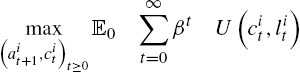
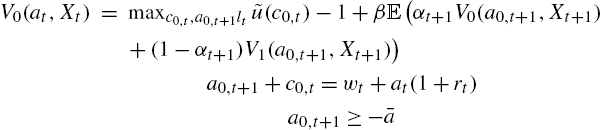
The typical problem of an agent facing incomplete insurance markets is the following
(1)
(2)
(3)
(4)
where ![]() is the wage rate in period t and
is the wage rate in period t and ![]() is the return on saving between period
is the return on saving between period ![]() and period t.
and period t. ![]() is the saving of agent i in period t, and
is the saving of agent i in period t, and ![]() are respectively the consumption and labor supply of agent i in period t. More rigorously, aggregate variables should be understood as a function of the history of aggregate shock
are respectively the consumption and labor supply of agent i in period t. More rigorously, aggregate variables should be understood as a function of the history of aggregate shock ![]() , thus as
, thus as ![]() and
and ![]() , whereas idiosyncratic variables should be understood as functions of both aggregate and idiosyncratic histories, as
, whereas idiosyncratic variables should be understood as functions of both aggregate and idiosyncratic histories, as ![]() for instance. The decisions in each period are subject to the non-negativity constraints (3). Importantly, agents can't borrow more than the amount
for instance. The decisions in each period are subject to the non-negativity constraints (3). Importantly, agents can't borrow more than the amount ![]() in each period.
in each period.
Production. Markets are competitive and a representative firm produces with capital and labor. The production function is ![]() , where μ is the capital depreciation rate, and
, where μ is the capital depreciation rate, and ![]() is the technology level, which is affected by technology shocks. The first-order conditions of the firm imply that factor prices are
is the technology level, which is affected by technology shocks. The first-order conditions of the firm imply that factor prices are
and
where ![]() is the aggregate capital stock and
is the aggregate capital stock and ![]() is the aggregate labor supply.
is the aggregate labor supply.
The technology shock is defined as the standard AR(1) process ![]() , with
, with
with ![]() .
.
2.2 Equilibrium Definition and Intuition to Reduce the State Space
We can provide the equilibrium definition and the main idea to reduce the state space. First, in the general case, as time goes by, there is an increasing number of different agents, due to the heterogeneity in idiosyncratic histories. Instead of thinking in sequential terms (i.e. following the history of each agent from period 0 to any period t), Huggett (1993) and Aiyagari (1994) have shown that the problem can be stated in recursive form, if ones introduces an infinite-support distribution as a state variable, when there are no aggregate shocks.2
Indeed, define as ![]() the cross-sectional cumulative distribution over capital holdings and idiosyncratic states in period t. For instance,
the cross-sectional cumulative distribution over capital holdings and idiosyncratic states in period t. For instance, ![]() is the mass of employed workers having a wealth level less than d at the beginning of period t. In the general case, an equilibrium of this economy is 1) a policy rule for each agent solving its individual maximization problem, 2) factor prices that are consistent with the firm first-order conditions, 3) financial and labor markets clear for each period
is the mass of employed workers having a wealth level less than d at the beginning of period t. In the general case, an equilibrium of this economy is 1) a policy rule for each agent solving its individual maximization problem, 2) factor prices that are consistent with the firm first-order conditions, 3) financial and labor markets clear for each period ![]() :
:
(5)

where ![]() is the saving in period t of a household having initial wealth a and being in state
is the saving in period t of a household having initial wealth a and being in state ![]() , and
, and
(6)
and finally 4) a law of motion for the cross-sectional distribution ![]() that is consistent with the agents' decision rule at each date. This law of motion can be written as (following the notation of Algan et al., 2014)
that is consistent with the agents' decision rule at each date. This law of motion can be written as (following the notation of Algan et al., 2014)
The literature on heterogeneous-agent models has tried to find solution techniques to approximate the very complex object ϒ, which maps distribution and shocks into distributions (Den Haan, 2010 for a presentation and discussion of differences in methods).
The basic idea. The basic idea for reducing the state space is first to go back to the sequential representation. If at any period t, only the last N periods are necessary to know the wealth of any agent, then only the truncated history ![]() is necessary to “follow” the whole distribution of agents, in a sense made clear below. In this economy, there are only
is necessary to “follow” the whole distribution of agents, in a sense made clear below. In this economy, there are only ![]() different agents at each period, instead of a continuous distribution. This number can be large, but it is finite and all standard perturbation techniques can be applied.
different agents at each period, instead of a continuous distribution. This number can be large, but it is finite and all standard perturbation techniques can be applied.
The next section presents different types of equilibria in the literature. The first one is the no-trade equilibrium where ![]() , the second one is the reduced-heterogeneity equilibrium, and the last one is the general case for arbitrary N.
, the second one is the reduced-heterogeneity equilibrium, and the last one is the general case for arbitrary N.
3 No-Trade Equilibria
3.1 No-Trade Equilibria with Transitory Shocks
A first simple way to generate a tractable model is to consider environments that endogenously generate no-trade equilibria with transitory shocks. This class of equilibrium was introduced by Krusell et al. (2011) to study asset prices with time-varying idiosyncratic risk. Recent developments show that they can be useful for macroeconomic analysis. Indeed, this equilibrium structure can be applied to a subgroup of agents.
3.1.1 Assumptions
These equilibria are based on two assumptions. First, assets are in zero net supply and production only necessitates labor (![]() in the production function). The first consequence is that the total amount of saving must be equal to the total amount of borrowing among households. The second consequence is that the real wage is only the technology level in each period
in the production function). The first consequence is that the total amount of saving must be equal to the total amount of borrowing among households. The second consequence is that the real wage is only the technology level in each period ![]() . Second, it is assumed that the borrowing limit is 0,
. Second, it is assumed that the borrowing limit is 0, ![]() . As agents can't borrow, there are no assets in which agents can save:
. As agents can't borrow, there are no assets in which agents can save: ![]() for all agents i in any period t. These equilibria are not interesting for generating a realistic cross-section of wealth, but they can be interesting to investigate the behavior of the economy facing time-varying uninsurable risk. Indeed, the price of any asset is determined by the highest price than any agent is willing to pay.
for all agents i in any period t. These equilibria are not interesting for generating a realistic cross-section of wealth, but they can be interesting to investigate the behavior of the economy facing time-varying uninsurable risk. Indeed, the price of any asset is determined by the highest price than any agent is willing to pay.
Denoting {1} the employed agents and {0} the unemployed agents, one can now state the problem recursively. The value functions for employed and unemployed agents are (I write these functions with the time index to facilitate the reading, although it is not necessary in this recursive formulation).
and
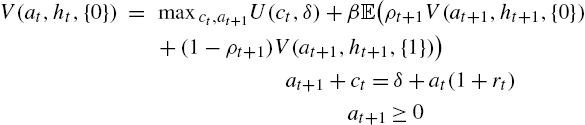
where the expectation operator ![]() is taken for the aggregate shock h only.
is taken for the aggregate shock h only.
As no agent can save, we have ![]() for all agents, and one can thus see that all employed agents consume
for all agents, and one can thus see that all employed agents consume ![]() and supply the same quantity of labor
and supply the same quantity of labor ![]() , whereas unemployed agents simply consume
, whereas unemployed agents simply consume ![]() and the labor supply is obviously given by
and the labor supply is obviously given by ![]() .
.
The equilibrium can be derived using a guess-and-verify structure. Indeed, for general values of the parameters derived below, unemployed agents are credit-constrained: they would like to borrow, and employed agents would like to save. As a consequence, they are the marginal buyer of the asset (although in zero-net supply) and make the price.
Deriving the first-order conditions of the previous program and then using these values, one finds

and the conditions for unemployed agents to be credit-constrained at the current interest rate is
Specification of the functional forms. Assume that
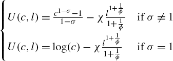
σ is the curvature of the utility function (not directly equal to risk aversion to the endogenous labor supply), and ϕ is the Frisch elasticity of labor supply, ranging from 0.3 to 2 in applied work (see Chetty et al., 2011 for a discussion). χ is a parameter scaling the supply of labor in steady state. With this specification one finds
(7)

and the conditions for unemployed agents to be credit-constrained at the current interest rate is
From the budget constraint of employed agents ![]() and the labor choice in (7), we obtain
and the labor choice in (7), we obtain
The technology process is the following
where ![]() is an AR(1) process specified above.
is an AR(1) process specified above.
Assume that three shocks hit the economy: A shock to the technology level, ![]() , a shock to the probability to stay employed
, a shock to the probability to stay employed ![]() and a shock to the probability to stay unemployed
and a shock to the probability to stay unemployed ![]() , which are AR(1) processes. More formally,
, which are AR(1) processes. More formally,
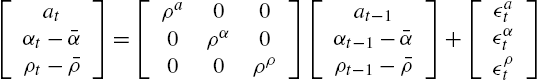
where the innovations ![]() ,
, ![]() , and
, and ![]() are white noise with standard deviation equal to
are white noise with standard deviation equal to ![]() ,
, ![]() , and
, and ![]() respectively,
respectively, ![]() . In the previous processes, the covariation between the exogenous shocks are 0, but alternative specifications are easy to introduce. The steady-state value of
. In the previous processes, the covariation between the exogenous shocks are 0, but alternative specifications are easy to introduce. The steady-state value of ![]() is
is ![]() and the steady-sate level of
and the steady-sate level of ![]() is
is ![]() .
.
Steady state. To use perturbation methods, we first solve for the steady sate and then consider first-order deviation from the steady state. In steady state ![]() , and we get from the two equations in (7),
, and we get from the two equations in (7),
(8)
and
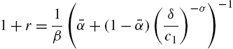
Putting in some numbers allows estimating the order of magnitude. Consider the period to be a quarter. The previous equality shows that the effect of uninsurable risk on the interest rate is the consumption inequality between employed and unemployed agents (irrespective of labor-supply elasticity for instance). Chodorow-Reich and Karabarbounis (2014) estimate a decrease in consumption of non-durable goods of households falling into unemployment between 10% and 20%. As a consequence, one can take the conservative value ![]() . The quarterly job loss probability is roughly 5% and
. The quarterly job loss probability is roughly 5% and ![]() (see Challe and Ragot, 2016 for a discussion), and the discount factor is
(see Challe and Ragot, 2016 for a discussion), and the discount factor is ![]() . One finds a real interest rate
. One finds a real interest rate ![]() for
for ![]() , and
, and ![]() when
when ![]() . In the complete market case, we have
. In the complete market case, we have ![]() and
and ![]() . We find
. We find ![]() . As is well known, market incompleteness contributes to a smaller steady-state interest rate compared to the complete market case (see Aiyagari, 1994 for a discussion).
. As is well known, market incompleteness contributes to a smaller steady-state interest rate compared to the complete market case (see Aiyagari, 1994 for a discussion).
3.2 Preserving Time-Varying Precautionary Saving in the Linear Model
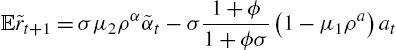
The effect of time-varying precautionary saving is preserved in the linear model for all the environments studied in this chapter. This is best understood in this simple framework. I denote by ![]() the proportional deviation of the variable x and by
the proportional deviation of the variable x and by ![]() the level deviation of variables y (applied typically to interest rate and transition probabilities). For instance,
the level deviation of variables y (applied typically to interest rate and transition probabilities). For instance, ![]() and
and ![]() . Linearizing the Euler equation in (7), one finds that
. Linearizing the Euler equation in (7), one finds that
(9)
where
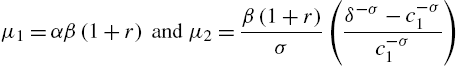
With the values given above, one finds ![]() and
and ![]() , when
, when ![]() . To give an order of magnitude, an increase in 10% in the expected job-separation rate (a decrease in α) has the same effect as an increase of 1% in the real interest rate. A second key implication is the value of
. To give an order of magnitude, an increase in 10% in the expected job-separation rate (a decrease in α) has the same effect as an increase of 1% in the real interest rate. A second key implication is the value of ![]() in front of
in front of ![]() . This has dramatic implications for monetary policy compared to the complete market case, where we have
. This has dramatic implications for monetary policy compared to the complete market case, where we have ![]() . These implications are studied by McKay et al. (2016) in this type of environment, to study forward guidance.
. These implications are studied by McKay et al. (2016) in this type of environment, to study forward guidance.
One can see that the probability to stay employed ![]() has a first-order effect on the consumption decision in (9) when markets are incomplete. The reason for this result is that we are not linearizing around a riskless steady state. We are linearizing around a steady state where idiosyncratic risk is preserved. As a consequence, there are two different marginal utilities that agents can experience in the steady state: either
has a first-order effect on the consumption decision in (9) when markets are incomplete. The reason for this result is that we are not linearizing around a riskless steady state. We are linearizing around a steady state where idiosyncratic risk is preserved. As a consequence, there are two different marginal utilities that agents can experience in the steady state: either ![]() if employed, or
if employed, or ![]() if unemployed. As a consequence, the term
if unemployed. As a consequence, the term ![]() in
in ![]() represents the lack of insurance in steady state. This term scales the reaction of consumption to changes in the idiosyncratic probability to switch employment status. In the complete market case, we obviously have
represents the lack of insurance in steady state. This term scales the reaction of consumption to changes in the idiosyncratic probability to switch employment status. In the complete market case, we obviously have ![]() .
.
Linearizing the labor-supply equation, one finds ![]() . Plugging this expression into (9), one finds that the value of the interest rate is pinned down by the shocks (using
. Plugging this expression into (9), one finds that the value of the interest rate is pinned down by the shocks (using ![]() and
and ![]() ):
):
One observes that an increase in the uncertainty (decrease in ![]() ) generates a fall in the expected real interest rate. Indeed, employed agents want to self-insure more in this case, and they accept a lower remuneration of their savings. An increase in productivity
) generates a fall in the expected real interest rate. Indeed, employed agents want to self-insure more in this case, and they accept a lower remuneration of their savings. An increase in productivity ![]() also decreases the expected real interest rate, as agents also want to self-insure more to transfer income from today to the next-period state of the world where they are unemployed.
also decreases the expected real interest rate, as agents also want to self-insure more to transfer income from today to the next-period state of the world where they are unemployed.
These no-trade equilibria are extreme representations of market incompleteness, as the consumption levels are exogenous. They can nevertheless be useful in DSGE models. For instance, Ravn and Sterk (2013) use the same trick to study an incomplete-insurance market model where households can be either employed or unemployed. The simplification on the households side allows to enrich the production side and to consider sticky prices, introducing quadratic costs of price adjustment à la Rotemberg, search-and-matching frictions on the labor market and downward nominal wage rigidities. In this environment, Ravn and Sterk consider two types of unemployed workers who differ in their search efficiency and therefore in their job-finding probabilities. They use this model to account for changes in the US labor market after the great recession. They focus in particular on the distinction of shifts in the Beveridge curve and of movements along the Beveridge curve. Werning (2015) uses this model to derive theoretical results about the effect of market incompleteness. Challe (2017) uses a no-trade equilibrium to analyze optimal monetary policy with sticky prices on the goods market and search-and-matching frictions on the labor market. He shows that optimal monetary policy reaction is more expansionary after a cost-push shock when markets are incomplete (compared to the complete market environment), because there are additional gains to reduce unemployment when markets are incomplete. McKay and Reis (2016a) analyze optimal time-varying unemployment insurance using this setup.
3.3 No-Trade Equilibrium with Permanent Shocks
A second line of literature to generate tractable no-trade equilibria is based on the Constantinides and Duffie (1996) environment. These authors consider permanent idiosyncratic risk (instead of transitory risk as in the previous framework) and show that one can study market allocations and asset prices with no-trade. Recently, Heathcote et al. (2014) generalized this framework to quantify risk-sharing and to decompose inequality into life-cycle shocks versus initial heterogeneity in preferences and productivity. Closed-form solutions are obtained for equilibrium allocations and for moments of the joint distribution of consumption, hours, and wages.
These no-trade equilibria are useful to provide a first quantification of new mechanisms generated by incomplete insurance markets. Nevertheless, they can't consider the macroeconomic effect of changes in savings after aggregate shocks. Small-heterogeneity models have been developed to consider this important additional channel in tractable environments.
4 Small-Heterogeneity Models
Small-heterogeneity models are classes of equilibria where agents do save but where the equilibrium distribution of wealth endogenously features a finite state space. Three classes of equilibria can be found in the literature. Each type of equilibrium has its own merit according to the question under scrutiny. I present the first one in detail, and the two others more rapidly, as the algorithms to solve for the equilibrium are very similar. The last class of equilibrium may be more suited for quantitative analysis, as the conditions for the equilibrium to exist are easier to check.
4.1 Models Based on Assumptions About Labor Supply
4.1.1 Assumptions
The first class of equilibria is based on two assumptions.
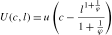
First, it is assumed that agents choose their labor supply when employed and that the disutility of labor supply is linear. If c is consumption and l is labor supply, the period utility function is
The implication of this assumption is that the first-order condition for labor supply pins down the marginal utility of consumption of employed agents. This assumption is used in Scheinkman and Weiss (1986) and in Lagos and Wright (2005) to simplify heterogeneity in various environments.
The second assumption is that the credit constraint is tighter than the natural borrowing limit
(10)
where r is the steady-state interest rate. This concept is introduced by Aiyagari (1994), and it is the loosest credit constraint, which ensures that consumption is always positive. The implication of this assumption is that unemployed agents will hit the credit constraint after a finite number of periods of unemployment. This property is key to reduce the state space, and we discuss it below.
4.1.2 Equilibrium Structure
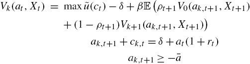
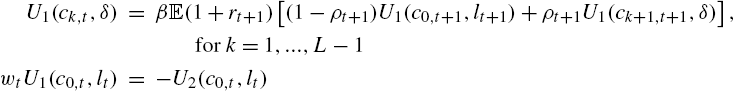
To simplify the exposition, the equilibrium is presented using a guess-and-verify strategy. For the sake of clarity, the time index is kept to variables (although not necessary in the recursive exposition). Assume that all employed agents consume and save the same amount in each period t, ![]() and
and ![]() respectively. In addition, assume that all agents unemployed for k periods consume and save the same amount, denoted
respectively. In addition, assume that all agents unemployed for k periods consume and save the same amount, denoted ![]() and
and ![]() , for
, for ![]() respectively. In addition, assume that agents unemployed for L periods are credit-constrained, and that this number is not time-varying (L is an equilibrium object). This last assumption is important and will be justified below.
respectively. In addition, assume that agents unemployed for L periods are credit-constrained, and that this number is not time-varying (L is an equilibrium object). This last assumption is important and will be justified below.
Denote as ![]() the value function of agents in state
the value function of agents in state ![]() (0 is employed agents, here), where
(0 is employed agents, here), where ![]() is the set of variables specified below that are necessary to form rational expectations.3
is the set of variables specified below that are necessary to form rational expectations.3
We have for employed people
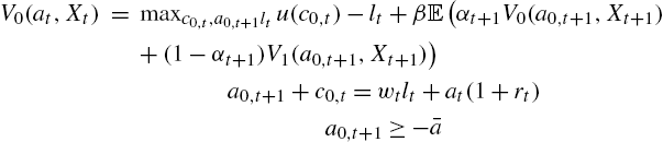
and for all unemployed people, ![]()

As credit constraints bind for agents unemployed for ![]() periods, we have for these agents
periods, we have for these agents ![]() .
.
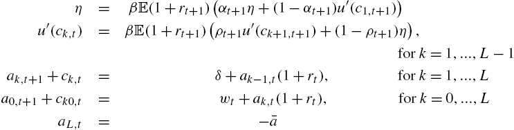
We can derive the set of first-order conditions. For employed agents

For unemployed agents, for ![]() .
.
Note that when ![]() , such that the credit constraints bind after one period of unemployment, then the previous equations don't exist. This case is studied more precisely below.
, such that the credit constraints bind after one period of unemployment, then the previous equations don't exist. This case is studied more precisely below.
The conditions define a system of ![]() equations.
equations.

These equations form a system in the ![]() variables
variables ![]() . These equations confirm the intuition that all employed agents consume and save the same amount.
. These equations confirm the intuition that all employed agents consume and save the same amount.
How is this possible? This comes from the labor choice, which provides some insurance. Indeed, as soon as an unemployed agent for k period in period ![]() becomes employed in period t, then they work the necessary amount, denoted as
becomes employed in period t, then they work the necessary amount, denoted as ![]() to consume
to consume ![]() . This amount is given by the budget constraint of employed households
. This amount is given by the budget constraint of employed households
(11)
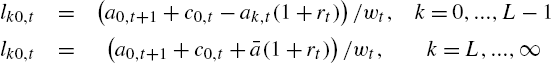
(The previous equation is indeed valid for ![]() .) Finally, note that for agents
.) Finally, note that for agents ![]() , we simply have, from the budget constraint
, we simply have, from the budget constraint
Thanks to the assumption about the credit constraint given by (3) and the assumption of small aggregate shocks (to use perturbation methods), this amount will be positive.
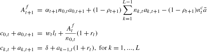
This almost concludes the description of the agent's decision. The last step is to follow the number of employed and of each type of unemployed agent. Denote as ![]() the number of agents in state
the number of agents in state ![]() in each period t. We have the law of motion of each type of agent
in each period t. We have the law of motion of each type of agent
The first equation states that the number of employed agents is equal to the number of employed agents who keep their job (first) term, plus the number of unemployed agents, which is ![]() , who find a job. The second equation states that the number of agents unemployed for k periods at date t, are the number of agents unemployed for
, who find a job. The second equation states that the number of agents unemployed for k periods at date t, are the number of agents unemployed for ![]() periods at the previous date who stay unemployed.
periods at the previous date who stay unemployed.
The number of k0 agents (i.e. employed agents at date t, who were unemployed for k periods at date ![]() ) is
) is
The number of credit-constrained agents is denoted as ![]() and is simply
and is simply

In this equilibrium, the capital market equilibrium is simply

and
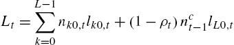
Here we used the fact that all constrained agents work the same amount when they find a job, due to condition (11).
Due to this assumption, the marginal utility of all employed agents is ![]() in all periods. As a consequence, this marginal utility does not depend on the history of agents on the labor market, what considerably simplifies the equilibrium structure.
in all periods. As a consequence, this marginal utility does not depend on the history of agents on the labor market, what considerably simplifies the equilibrium structure.
4.1.3 The System
We can now present the whole system of equations:
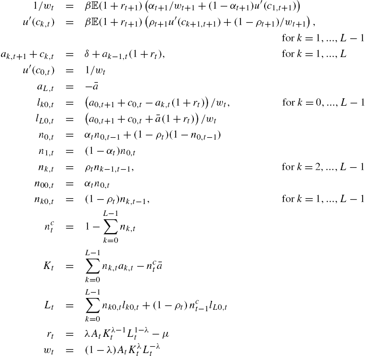
This system is large but finite. There are ![]() equations for
equations for ![]() variables
variables ![]() . For any process for the exogenous shocks
. For any process for the exogenous shocks ![]() one may think that it is possible to simulate this model. This is not the case because one key variable is not determined: L.
one may think that it is possible to simulate this model. This is not the case because one key variable is not determined: L.
4.1.4 Algorithm: Finding the Value of L
The value of L can be found using steady-state solutions of the previous system. The idea is to find the steady-state for any L and iterate over L to find the value for which L agents are credit constrained, whereas ![]() agents are not. The algorithm to find L and the steady state is the following (finding the steady state is not difficult because the problem is block-separable). I simply drop the time subscript to denote steady-state values.
agents are not. The algorithm to find L and the steady state is the following (finding the steady state is not difficult because the problem is block-separable). I simply drop the time subscript to denote steady-state values.
Algorithm
- 1. Take
 as given.
- a. Take r as given.
- i. From r deduce w using the FOCs of the firms.
- ii. Solve for the consumption of agents
 using the Euler equations of the agents, from
  to
to  .
. - iii. Solve for the saving of the agents from
 down to
  using the budget constraint of all agents, and the values .
 - iv. Solve for the labor supply of employed agents

 .
. - v. Solve for the share of agents
 for
for  and
and  .
. - vi. Find the aggregate capital stock K.
- b. Iterate over r, until the financial market clears, i.e. until
 .
.
- a. Take r as given.
- 2. Iterate over L, until
(12)
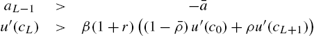
- where
 .
.
4.1.5 Simulations
Once the steady-state value of L and the steady-state value of the variables are determined, one can simulate the model using standard perturbation methods. One can use DYNARE to simulate first and second approximations of the model, compute second moments, and so on. The distribution of wealth is summarized by the vector ![]() and belongs to the state space of agents
and belongs to the state space of agents ![]() to form rational expectations. In these simulations, one has to check that the aggregate shock is small enough such that L is indeed constant over time. One must thus check that the condition (12) is satisfied not only in the steady state but also during the simulations.
to form rational expectations. In these simulations, one has to check that the aggregate shock is small enough such that L is indeed constant over time. One must thus check that the condition (12) is satisfied not only in the steady state but also during the simulations.
4.1.6 References and Limits
In the Bewley–Huggett–Aiyagari environment, Algan et al. (2011) use this framework to investigate the impact of money injections in a model where agents use money to self-insure against idiosyncratic shocks. Challe et al. (2013) use this assumption to study the effect of an increase in public debt on the yields curve in an environment where agents use safe assets of various maturities to self-insure against idiosyncratic risk. They show that an increase in idiosyncratic risk decreases both the level and the slope of the yield curve. In addition, an increase in public debt increases both the level and the slope of the yield curve. LeGrand and Ragot (2016a) use this assumption to consider insurance for aggregate risk in these environments. Introducing derivative assets, such as options, in an environment where agents use a risky asset to self-insure against idiosyncratic risk, they show that the time-variations in the volume of traded derivative assets are consistent with empirical findings.
This framework is interesting to investigate the properties of time-varying precautionary saving in finance (for instance to study asset prices) but it is not well suited for the macroeconomy. Indeed, the elasticity of labor supply is much too high compared to empirical findings (the Frisch elasticity is here infinite, whereas it is between 0.3 and 1 in the data, see Chetty et al., 2011 for a discussion). In addition, all employed agents consume the same amount, which is pinned down by the real wage, which is obviously a counterfactual. For this reason, other frameworks with positive trade have been developed.
4.2 Models Based on Linearity in the Period Utility Function
Challe and Ragot (2016) present an alternative environment, consistent with any value of the elasticity of the labor supply. This framework can thus be used in macroeconomic environments to model time-varying movements in inequality. We describe the empirical relevance and the modeling strategy in Section 4.2.3 after the presentation of the model.
4.2.1 Assumptions
The model relies on three assumptions.
First, instead of introducing linearity in the labor supply, the linearity is in the utility of consumption. More precisely, it is assumed that there exists a threshold ![]() such that the period utility function is strictly concave for
such that the period utility function is strictly concave for ![]() and linear for
and linear for ![]() . The linear-after-a-threshold utility function was introduced by Fishburn (1977) in decision theory to model behavior in front of gains and losses differently.
. The linear-after-a-threshold utility function was introduced by Fishburn (1977) in decision theory to model behavior in front of gains and losses differently.
The period utility function is thus
(13)

where the function ![]() is increasing and concave. The slope of the utility function must be low enough to obtain global concavity, that is
is increasing and concave. The slope of the utility function must be low enough to obtain global concavity, that is ![]() .
.
Second, the borrowing limit is assumed to be strictly higher than the natural borrowing limit, as before.
Third, it is assumed that the discount factor of agents is such that all employed agents consume an amount ![]() and all unemployed agents consume an amount
and all unemployed agents consume an amount ![]() .
.
4.2.2 Equilibrium Structure
To save some space, we now focus on the households' program. Assume that labor is inelastic as a useful benchmark (introducing elastic labor is very simple in this environment). All employed agents supply one unit of labor.
We have for employed people
and for all unemployed people, ![]()
One can solve for the order conditions following the same steps as before. Using the same notations as in the previous section, denote as k agents the agents unemployed for k periods. Assuming that credit constraints are binding after L periods of unemployment, one can find consumption and saving choices.
The key difference between this environment and the one presented in the previous section is that employed agents will not differ according to their labor supply (which is inelastic), but by their consumption level. Denote as ![]() the consumption at date t of employed agents who were unemployed for k periods at date
the consumption at date t of employed agents who were unemployed for k periods at date ![]() , and denote (as before) as
, and denote (as before) as ![]() (for
(for ![]() ) the consumption of unemployed agents who are unemployed for k periods at date t. The households are now described by the vector
) the consumption of unemployed agents who are unemployed for k periods at date t. The households are now described by the vector ![]() and
and ![]() solving
solving
One can check that this is a system of ![]() equations for
equations for ![]() variables. The number of each type of agent can be followed as in the previous section.
variables. The number of each type of agent can be followed as in the previous section.
One may find this environment more appealing than the one in the previous section, as it does not rely on an unrealistic elasticity of labor supply. The problem is nevertheless that there are additional conditions for the equilibrium existence that limit the use of such a framework. Indeed, one has first to solve for steady-state consumption and savings for each type of agent, and for the steady-state value of L using the algorithm described in Section 4.1.4, and then one has to check the following ranking condition:
The previous condition is that the highest steady-state consumption of unemployed agents is lower than the lowest steady-state consumption of employed agents. Indeed, the consumption of households just becoming unemployed (and thus being employed in the previous period) ![]() is the highest consumption of unemployed agents, because consumption is falling with the length of the unemployment spell. Moreover, the consumption of employed agents who were at the credit constraint in the previous period,
is the highest consumption of unemployed agents, because consumption is falling with the length of the unemployment spell. Moreover, the consumption of employed agents who were at the credit constraint in the previous period, ![]() , is the lowest consumption level of employed agents, because these agents have the lowest beginning-of-period wealth
, is the lowest consumption level of employed agents, because these agents have the lowest beginning-of-period wealth ![]() . If the condition is fulfilled, one can always find a threshold
. If the condition is fulfilled, one can always find a threshold ![]() such that the period utility function is well behaved.
such that the period utility function is well behaved.
This framework can nevertheless be used in realistic dynamic models when applied to a subgroup of the population.
4.2.3 Using Reduced Heterogeneity to Model Wealth Inequality over the Business Cycle
Challe and Ragot (2016) apply the previous framework to model the bottom 60% of US households, based on the following observation. The wealth share of the poorest 60% of households in terms of liquid wealth is as low as 0.3%. Indeed, as the model is used to model precautionary saving in the business cycle, one should indeed focus on the net worth, which can readily be used for the short-run change in income. Define the period to be a quarter.
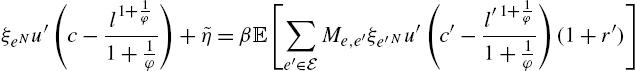
The modeling strategy is the following. Challe and Ragot (2016) model the top 40% of the households by a family, that can fully insure its members against unemployment risk. This family has a discount factor ![]() for patient and it has thus a standard Euler equation (without the employment risk, which is insured).
for patient and it has thus a standard Euler equation (without the employment risk, which is insured).
As a consequence, the bottom 60% is modeled by agents having a quasi-linear utility function and having a lower discount factor, denoted as ![]() (I for impatient, P for patient). With such a low wealth shares of 0.3% (a few hundred dollars of savings), it is easy to show that the households spend all their saving after a quarter of unemployment. This implies that one can construct an equilibrium for the bottom, where
(I for impatient, P for patient). With such a low wealth shares of 0.3% (a few hundred dollars of savings), it is easy to show that the households spend all their saving after a quarter of unemployment. This implies that one can construct an equilibrium for the bottom, where ![]() . In other words, these households face the credit constraint after one period (one quarter) of unemployment.
. In other words, these households face the credit constraint after one period (one quarter) of unemployment.
The inter-temporal choice of employed agents can be simply written as
where we used the fact that ![]() .
.
One can linearize the previous equation to obtain a simple saving rule. Level-deviations from the steady state are denoted with a tilde, as before. Linearization gives
where ![]() are coefficients that depend on parameter values. One can show that
are coefficients that depend on parameter values. One can show that ![]() , because agents facing a higher probability to stay employed decrease their precautionary savings. The coefficient
, because agents facing a higher probability to stay employed decrease their precautionary savings. The coefficient ![]() can be either positive or negative depending on parameter values, and on income and substitution effects.
can be either positive or negative depending on parameter values, and on income and substitution effects.
Due to the saving rule, the model differs from hand-to-mouth DSGE models in the tradition of Kiyotaki and Moore (1997). In the previous model, the number of credit-constrained agents is very low, as households at the constraint are the fraction of impatient agents who are unemployed and not the full population of impatient agents. Finally, the conclusion of this model that poor households (the bottom 60% of the wealth distribution) react more to the unemployment risk than rich households is confirmed by household data (see Krueger et al., 2015). As a consequence, this framework is empirically more relevant than the no-trade equilibria presented above, or hand-to-mouth models following the seminal paper of Kiyotaki and Moore (1997).
Finally, Challe and Ragot (2016) show that this model does a relatively good job in reproducing time-varying precautionary saving (compared to Krusell and Smith, 1998), and that the model is not more complicated than a standard DSGE model. In particular, it can be solved easily using DYNARE.
4.2.4 Other References and Remarks
LeGrand and Ragot (2016c) extend this environment to introduce various segments in the period utility function to consider various types of agents. They apply this framework to show that such a model can reproduce a rich set of empirical moments when limited participation in financial markets is introduced. In particular, the model can reproduce the low risk free rate, the equity premium the volatility of the consumption growth rate of the top 50% together with the aggregate volatility of consumption.
The use of a quasi-linear utility function provides (with the relevant set of assumptions) a simple representation of household heterogeneity focusing on the poor households who indeed face a higher unemployment risk. The cost of this representation is that the existence conditions can be violated for big aggregate shocks or for an alternative calibration of the share of households facing the unemployment risk. As a consequence, this representation is not well-suited for Bayesian estimation, as it is not sure that existence conditions are fulfilled for any samples. To overcome this difficulty, other assumptions can be introduced.
4.3 Models Based on a “Family” Assumption
The modeling strategy of previous models is based on the reduction of the state space by 1) reducing heterogeneity among high-income agents and 2) setting the credit constraints at a level higher than the natural borrowing limit (to be sure that low-income households reach the credit limit in a finite number of periods). The two previous modeling strategies played with utility functions to reach this goal. The last modeling strategy follows another route and considers directly different market arrangements for any utility function. It will be assumed that there is risk-sharing among employed agents. The presentation follows Challe et al. (2017), but it is much simpler because we do not introduce habit formation.
4.3.1 Assumptions
The model is based on limited insurance (“or the family assumption”) often used in macro, but applied to a subgroup of agents. Assume that all agents belong to a family. The family head cares for all agents, but has a limited ability to transfer resources across agents. Indeed, the planner can transfer resources across agents on the same islands, but it cannot transfer resources across islands. More specifically:
- 1. All employed agents are on the same islands, where there is full risk-sharing.
- 2. All unemployed agents for k periods live on the same island, where there is full risk-sharing.
- 3. A representative of the family head implements the consumption-saving choice in all islands, maximizing total welfare.
- 4. The representative of the family head choose allocate wealth to households before knowing their next-period employment status.
The structure can be seen as a deviation from Lucas (1990) to reduce heterogeneity among employed agents. It will generate the same structure as the previous models: no heterogeneity among employed agents and heterogeneous unemployed agents according to the length of their unemployment spell.
4.3.2 Equilibrium Structure
As before, we use a guess-and-verify strategy to present the model. Assume that the unemployed agents reach the credit constraint after L consecutive periods of unemployment.
As before, denote as ![]() the number of employed agents at date t, and as
the number of employed agents at date t, and as ![]() the number of agents unemployed for
the number of agents unemployed for ![]() consecutive periods at date t. Denote as
consecutive periods at date t. Denote as ![]() the value function of the family head, and
the value function of the family head, and ![]() as the value function of households unemployed for k periods. First, the value function of agents in the employed island is
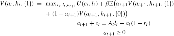
as the value function of households unemployed for k periods. First, the value function of agents in the employed island is

Let's explain this problem. The family head maximizes the utility of all agents in the employed island (imposing the same consumption and labor choice on all agents to maximize welfare). The head takes into consideration the fact that some employed agents will fall into unemployment next period (and will have the value function ![]() which is the inter-temporal welfare of agents unemployed for one period). The budget constraint is written in per capita terms: Per capita income is equal to per capita consumption and per capita savings, denoted as
which is the inter-temporal welfare of agents unemployed for one period). The budget constraint is written in per capita terms: Per capita income is equal to per capita consumption and per capita savings, denoted as ![]() . At the end of the period, all agents in the employed island have the same wealth, which is
. At the end of the period, all agents in the employed island have the same wealth, which is ![]() . As the family head cannot discriminate between agents before they leave the island, this will be the next-period beginning-of-period wealth of agents leaving the island, i.e. just falling into unemployment.
. As the family head cannot discriminate between agents before they leave the island, this will be the next-period beginning-of-period wealth of agents leaving the island, i.e. just falling into unemployment.
Finally, the next-period wealth of employed agents is the next-period pooling of the wealth of agents staying or becoming employed. First, it sums the wealth of agents staying employed ![]() , and the wealth of unemployed agents not at the credit constraint in period t and finding a job in period
, and the wealth of unemployed agents not at the credit constraint in period t and finding a job in period ![]() ,
, ![]() , and the wealth of agents constrained in period t and finding a job in period
, and the wealth of agents constrained in period t and finding a job in period ![]() . These agents have a wealth
. These agents have a wealth ![]() (recall that
(recall that ![]() is the number of agents at the credit constraint in period t).
is the number of agents at the credit constraint in period t).
The value function of unemployed agents for k periods is simpler
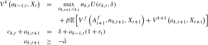
In this maximization, the representative of the family head in the island where agents are unemployed for k periods takes into account the fact that they will affect the next-period wealth of employed agents, because all agents belong to a whole family, and the wealth of agents unemployed for ![]() periods, in the next period. First-order and envelope conditions for employed agents are
periods, in the next period. First-order and envelope conditions for employed agents are

First-order and envelope conditions for unemployed agents are

Combining these equations (and using the fact that ![]() and
and ![]() ), one finds the set of equations defining the agents' choice.
), one finds the set of equations defining the agents' choice.
(14)
(15)
(16)
Given the prices ![]() and
and ![]() , this is a system of
, this is a system of ![]() equations for the
equations for the ![]() variables
variables ![]() . The key result of this construction is that the Euler equations of employed and unemployed agents are the same as those obtained in a model with uninsurable idiosyncratic risk. Indeed, using the law of large numbers (which is assumed to be valid in a continuum), the “island” metaphor transforms idiosyncratic probabilities into shares of agents switching between islands. The gain is that the state space is finite and the amount of heterogeneity is finite, as there are only
. The key result of this construction is that the Euler equations of employed and unemployed agents are the same as those obtained in a model with uninsurable idiosyncratic risk. Indeed, using the law of large numbers (which is assumed to be valid in a continuum), the “island” metaphor transforms idiosyncratic probabilities into shares of agents switching between islands. The gain is that the state space is finite and the amount of heterogeneity is finite, as there are only ![]() different wealth levels.
different wealth levels.
Note that the consumption of ![]() for
for ![]() is
is ![]() because
because ![]() for
for ![]() .
.
The capital stock and total labor supply are simply

Compared to the environments in Section 4.1 and in Section 4.2, the current equilibrium exhibits less heterogeneity, as all employed agents consume and work the same amount. The gain is that the period utility function can be very general.
4.3.3 Algorithm and Simulations
The algorithm to find the steady state is the following.
- 1. Guess a value for .
- 2. Guess a value for r; from r deduce w using the FOCs of the firms.
- 3. Guess a value for
 ; deduce the labor supply using (15).
 - a. Solve for the consumption of agents using the Euler equations of the agents, from
 to
to  .
. - b. Solve for the saving of the agents from to using the budget constraint of all agents, and the values .
- c. Solve for the share of agents
 for and .
 - d. Find the aggregate capital stock K and aggregate labor L.
- a. Solve for the consumption of agents
- 4. Iterate on r, until the financial market clears, i.e. until .
- 5. Iterate on L, until
(17)
- where .
The model is again a finite set of equations, which can be simulated using DYNARE. The DYNARE solver could be used to double-check the values of the steady state.
4.3.4 Example of Quantitative Work
Challe et al. (2017) use this representation of heterogeneity to construct a full DSGE model with heterogeneous agents. Indeed, the authors assume that only the bottom 60% in the wealth distribution form precautionary saving, and that the top 40% can be modeled by a representative agent.
They then introduce many other features to build a quantitative model, such as 1) sticky prices, 2) habit formation (which complexifies significantly the exposition of the equilibrium), 3) capital adjustment costs, 4) search-and-matching frictions on the labor market, and 5) stochastic growth.
The general model is then brought to the data using Bayesian estimations. The information used in the estimation procedure includes thus the information set used to estimate DSGE models. In addition, information about time-varying consumption inequalities across agents can be used in the estimation process. The model is used to assess the role of precautionary saving during the great recession in the US. The authors show that a third of the fall in aggregate consumption can be attributed to time-varying precautionary saving due to the increase in unemployment during this period.
The possibility to use Bayesian estimation is a clear strength of this class of model. Indeed, as time-varying precautionary saving is preserved after linearization, the same techniques as in the representative-agent DSGE literature can be used, but lots of new data about time-varying moments of the distribution of income, wealth or consumption can be used to disciplined the model. This open the route for richer quantitative works.
4.4 Assessment of Small-Heterogeneity Models
The three classes of small-heterogeneity model presented in this section have the merit to keep the effects of time-varying precautionary savings using perturbation methods. Compared to no-trade equilibria, the actual quantity of assets used to self-insure, i.e. the optimal quantity of liquidity in the sense of Woodford (1990), is endogenous. In addition, this can easily be applied to a relevant subset of households in a DSGE model.
An additional gain of these representations is that the state space is small. For an equilibrium where agents hit the borrowing constraint after L periods of unemployment, there are only ![]() different wealth levels.
different wealth levels.
There are nevertheless two main drawbacks. First, when L grows, the state space doesn't converge toward a Bewley economy, because there is no heterogeneity across employed households. As a consequence, one cannot consider the full-fledged Bewley economy as the limit of these equilibria when there are no aggregate shocks. As a further consequence, one cannot use all the information about the cross-section of household inequality (for instance all employed agents are similar). Hence, the models capture only a part of time-varying precautionary saving. Admittedly, this a key part as the unemployment risk is the biggest uninsurable risk faced by households (Carroll et al., 2003).
The second drawback is that the number of periods of consecutive unemployment before the credit constraint binds (denoted as L) is part of the equilibrium definition: it has to be computed as a function of the model parameters. If aggregate shocks are small enough, this number is not time-varying, but this has to be checked during the simulations.
New developments provide environments without these drawbacks, at the cost of a bigger state space.
5 Truncated-History Models
LeGrand and Ragot (2016b) present a general model to generate limited heterogeneity with an arbitrarily large but finite state space and which can be made close to the Bewley model. In this environment, the heterogeneity across agents depends only on a finite but possibly arbitrarily large number, denoted N, of consecutive past realizations of the idiosyncratic risk (as a theoretical outcome). As a consequence, the history of idiosyncratic risk is truncated after N periods. Agents sharing the same idiosyncratic risk realizations for the previous N periods choose the same consumption and wealth. As a consequence, instead of having a continuous distribution of heterogeneous agents in each period, the economy is characterized by a finite number of heterogeneous consumption and wealth levels. The model can be simulated with DYNARE and optimal policy can be derived solving a Ramsey problem in this environment. The presentation follows the exposition of the decentralized equilibrium of LeGrand and Ragot (2016b).4
5.1 Assumptions
Truncated histories. Consider the following notations. First, the program is written in recursive forms to simplify the exposition, such that ![]() is the next-period value of the variable x.
is the next-period value of the variable x. ![]() is the current beginning-of-period idiosyncratic state of the agent under consideration,
is the current beginning-of-period idiosyncratic state of the agent under consideration, ![]() is the beginning-of-period idiosyncratic state one period ago, and
is the beginning-of-period idiosyncratic state one period ago, and ![]() is the beginning-of-period idiosyncratic state k periods ago. As a consequence and for any N, each agent enters any period with an N-period history
is the beginning-of-period idiosyncratic state k periods ago. As a consequence and for any N, each agent enters any period with an N-period history ![]() ,
, ![]() . This N-period history is a truncation of the whole history of each agent: It is the history of the agent for the last N periods, before the agent learns its current idiosyncratic shock
. This N-period history is a truncation of the whole history of each agent: It is the history of the agent for the last N periods, before the agent learns its current idiosyncratic shock ![]() for the current period.
for the current period.
After the idiosyncratic shock is realized, the agent has the ![]() -period history denoted
-period history denoted ![]() . Histories without a tilde are thus histories after the idiosyncratic shock is realized. We can also write
. Histories without a tilde are thus histories after the idiosyncratic shock is realized. We can also write ![]() . Indeed,
. Indeed, ![]() can be seen as the history
can be seen as the history ![]() with the successor state e, or as the state
with the successor state e, or as the state ![]() followed by the N-period history
followed by the N-period history ![]() .
.
The probability ![]() that a household with end-of-period history (i.e. after the idiosyncratic shock is realized)
that a household with end-of-period history (i.e. after the idiosyncratic shock is realized) ![]() in the current period experiences a next-period end-of-period history
in the current period experiences a next-period end-of-period history ![]() is the probability to switch from state
is the probability to switch from state ![]() in the current period to state
in the current period to state ![]() in the next period, provided that histories
in the next period, provided that histories ![]() and
and ![]() are compatible. More formally:
are compatible. More formally:
(18)
where ![]() if
if ![]() is a possible continuation of history
is a possible continuation of history ![]() , and 0 otherwise.
, and 0 otherwise.
From the expression (18) of the probability ![]() , we can deduce the dynamics of the number of agents having history
, we can deduce the dynamics of the number of agents having history ![]() in each period, denoted
in each period, denoted ![]() :
:
(19)

The previous expression is the application of the law of large numbers in a continuum.
Preferences. For quantitative reasons that will appear clear below, we assume that the utility of each agent may be affected by its idiosyncratic history. More formally, it depends on the history of idiosyncratic risk ![]() , recalling that
, recalling that ![]() . As a consequence, preference depends on the current and the last
. As a consequence, preference depends on the current and the last ![]() idiosyncratic shocks. The period utility is thus
idiosyncratic shocks. The period utility is thus ![]() , where
, where ![]() . The equilibrium can be derived for
. The equilibrium can be derived for ![]() , as in LeGrand and Ragot (2016b). Adding the terms
, as in LeGrand and Ragot (2016b). Adding the terms ![]() is a trick to make the model more quantitatively relevant. It has the same role as the stochastic discount factor in Krusell and Smith (1998).
is a trick to make the model more quantitatively relevant. It has the same role as the stochastic discount factor in Krusell and Smith (1998).
To simplify the algebra, it is assumed that the period utility function exhibits no wealth effect on the labor supply (which is consistent with empirical estimates). The period utility function is of the Greenwood–Hercowitz–Huffman (GHH) type
State vector. Denote by X the state vector in each period, which is necessary to form rational expectations. This state vector will be specified below. For now it is sufficient to assume that it is finite dimensional.
Transfer. The trick to reduce heterogeneity is to assume that each agent receives a lump-sum transfer, which depends on her ![]() -history. This lump-sum transfer is denoted
-history. This lump-sum transfer is denoted ![]() and it will be balanced in each period.
and it will be balanced in each period.
Program of the agents. The agent maximizes her inter-temporal welfare by choosing the current consumption c, labor effort l, and asset holding ![]() . She will have to pay an after-tax interest rate and wage rate denoted as r and w, as before. The value function can be written as
. She will have to pay an after-tax interest rate and wage rate denoted as r and w, as before. The value function can be written as
(20)

(21)
(22)
Denote by ![]() the Lagrange multiplier of the credit constraint
the Lagrange multiplier of the credit constraint ![]() . The solution to the maximization program (20)–(22) is the policy rules denoted
. The solution to the maximization program (20)–(22) is the policy rules denoted ![]() ,
, ![]() ,
, ![]() and the multiplier
and the multiplier ![]() satisfying the following first-order conditions, written in a compact form (I omit the dependence in X to lighten notations):
satisfying the following first-order conditions, written in a compact form (I omit the dependence in X to lighten notations):
(23)
(24)
(25)
(26)
5.2 Equilibrium Structure
We can show that all agents with the same current history ![]() have the same consumption, saving, and labor choices. To do so, we follow a guess-and-verify strategy. Assume that agents entering the period with a beginning-of-period history
have the same consumption, saving, and labor choices. To do so, we follow a guess-and-verify strategy. Assume that agents entering the period with a beginning-of-period history ![]() have the same beginning-of-period saving
have the same beginning-of-period saving ![]() . These agents have a current productivity shock e, and have thus a history
. These agents have a current productivity shock e, and have thus a history ![]() . There are
. There are ![]() agents with a beginning-of-period history
agents with a beginning-of-period history ![]() and
and ![]() agents with a current (i.e. after the current shock) history
agents with a current (i.e. after the current shock) history ![]() .
.
Under the assumption that for any ![]() , agents having the history
, agents having the history ![]() have the same beginning-of-period wealth
have the same beginning-of-period wealth ![]() , the average welfare (before transfer) of agents having a current N-period history is
, the average welfare (before transfer) of agents having a current N-period history is
(27)

The term ![]() is the total wealth of agents having current history
is the total wealth of agents having current history ![]() . Dividing by the number of those agents, we find the per capita value
. Dividing by the number of those agents, we find the per capita value ![]() . The transfer is now easy to define:
. The transfer is now easy to define:
(28)
The transfer ![]() swaps the remuneration of the beginning-of-period wealth
swaps the remuneration of the beginning-of-period wealth ![]() of agents having history
of agents having history ![]() by the remuneration of the average wealth
by the remuneration of the average wealth ![]() of agents having the current N-period history
of agents having the current N-period history ![]() . It is easy to see that this transfer is balanced, as it only reshuffles wealth across a sub-group of agents.
. It is easy to see that this transfer is balanced, as it only reshuffles wealth across a sub-group of agents.
The impact of the transfer on agents' wealth. It is easy to see that all agents consider the lump-sum transfer ![]() as given and thus do not internalize the effect of their choice on this transfer (because there is a continuum of agents for any truncated history). We consider the impact of transfer
as given and thus do not internalize the effect of their choice on this transfer (because there is a continuum of agents for any truncated history). We consider the impact of transfer ![]() for an agent with history
for an agent with history ![]() and beginning-of-period wealth
and beginning-of-period wealth ![]() . Her budget constraint (21) can be expressed using transfer expression (28) as follows:
. Her budget constraint (21) can be expressed using transfer expression (28) as follows:
(29)
The beginning-of-period and after-transfer wealth of agents with a beginning-of-period history ![]() depends only on the current N-period history
depends only on the current N-period history ![]() . Moreover, as can be seen from (20), agents with the same N-period history
. Moreover, as can be seen from (20), agents with the same N-period history ![]() are endowed with the same expected continuation utility as long as they save the same amount
are endowed with the same expected continuation utility as long as they save the same amount ![]() . Therefore, agents with the same current N-period history
. Therefore, agents with the same current N-period history ![]() behave similarly: they consume the same level, they supply the same labor quantity, and they hold the same wealth.
behave similarly: they consume the same level, they supply the same labor quantity, and they hold the same wealth.
State vector. The aggregate state of the economy X is the collection of: (i) the beginning-of-period wealth distribution depending on the N-period history ![]() (i.e., the size of the agent population with history
(i.e., the size of the agent population with history ![]() , together with their respective wealth), and (ii) the aggregate state h, which affects transition probabilities.
, together with their respective wealth), and (ii) the aggregate state h, which affects transition probabilities.
5.3 Equations of the Model
We can now write the equations of the models with a truncation for N periods of idiosyncratic histories. We introduce the time subscript to simplify the reading and the numerical implementation. Define as ![]() the set of N-period idiosyncratic histories for which agents face credit constraints (we show how to find
the set of N-period idiosyncratic histories for which agents face credit constraints (we show how to find ![]() below). The histories
below). The histories ![]() are thus not credit-constrained.
are thus not credit-constrained.
(30)
(31)
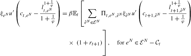
(32)
(33)
(34)

(35)

(36)

(37)
(38)
(39)
For a given technology process ![]() , this system has
, this system has ![]() equations for
equations for ![]() variables
variables ![]() . Before simulating the model, one has to find the set of histories facing credit constraint
. Before simulating the model, one has to find the set of histories facing credit constraint ![]() . To do so, we first solve the model under steady state to find
. To do so, we first solve the model under steady state to find ![]() , and then we assume that shocks are small enough to check that credit constraints are indeed binding.
, and then we assume that shocks are small enough to check that credit constraints are indeed binding.
5.4 Algorithm for the Steady State
For a given N, rank first the agents according to their idiosyncratic history. For instance, for the history ![]() N, one can consider
N, one can consider ![]() . With this ordering,
. With this ordering, ![]() for the agents who are unemployed for N periods
for the agents who are unemployed for N periods ![]() and
and ![]() for
for ![]() . In other words, agents with a low k have been unemployed recently for a long period of time. All the steady-state variables will be indexed by k instead of
. In other words, agents with a low k have been unemployed recently for a long period of time. All the steady-state variables will be indexed by k instead of ![]() . We thus look for
. We thus look for ![]() .
.
The algorithm for the steady state is the following.
- 1. Assume that the set of histories
 is credit constrained. For all
  , we have
  .
. - a. Consider an interest rate r such that
 . Deduce the real wage w, using Eqs. (38) and (39).
 - b. Deduce
 using (32).
- i. Assume values for the vector of consumption levels of constrained agents
 .
. - ii. Using the Euler equations (31) and labor supply find the consumption levels of unconstrained agents
 .
. - iii. Using the budget constraints (30) of unconstrained agents and the risk-sharing equation (34) find the savings of unconstrained agents
 .
. - iv. Deduce from the budget constraint of constrained agents,
 , the implied consumption levels
  .
. - v. Iterate over until
 .
.
- i. Assume values for the vector of consumption levels of constrained agents
- c. Compute the implied interest rate
 using Eqs. (36), (37), and (38).
 - d. Iterate on r until
 .
.
- a. Consider an interest rate r such that
- 2. Check that histories are credit-constrained and histories
 are not, iterate on otherwise.
5.5 Dynamics
The model can be easily simulated for small aggregate shocks at the first order, assuming that those shocks are small enough such that the set of constrained histories remains always the same. This can be checked during each simulation, checking that Euler equations hold with inequality for assumed constrained households. The simple way to simulate the model is 1) to write a code that writes the set of equations (30)–(39) as a DYNARE code, 2) specify the steady state found in the previous section as initial values to double-check that the steady state is correct, using the “resid” function of DYNARE, and 3) simulate the model using the “stoch_simul” function.
5.6 Choosing the Preference Shifters 
The simulations of the model can be done for any ![]() . How can we choose these parameters? What are they useful for? The simplest choice is to set
. How can we choose these parameters? What are they useful for? The simplest choice is to set ![]() . But the choice of these
. But the choice of these ![]() can be made to improve the fit of the equilibrium distribution to a given target. Indeed, if one has empirical average estimates of wealth levels of agents for an observed history on the labor market
can be made to improve the fit of the equilibrium distribution to a given target. Indeed, if one has empirical average estimates of wealth levels of agents for an observed history on the labor market ![]() , namely
, namely ![]() for
for ![]() , then one can iterate over
, then one can iterate over ![]() , until the steady savings values of the model are close enough to their empirical counterpart
, until the steady savings values of the model are close enough to their empirical counterpart ![]() for
for ![]() . For instance, one can simulate a Bewley–Aiyagari–Huggett model to get the model-generated averages
. For instance, one can simulate a Bewley–Aiyagari–Huggett model to get the model-generated averages ![]() for
for ![]() , and then iterate over
, and then iterate over ![]() in the truncated economy for the steady-state outcome of the truncated model to be close to the “true” values
in the truncated economy for the steady-state outcome of the truncated model to be close to the “true” values ![]() for
for ![]() . The general ability of the truncated model to reproduce any given wealth distribution is still an open question.
. The general ability of the truncated model to reproduce any given wealth distribution is still an open question.
5.7 Numerical Example
As an example, one can now provide numerical simulations of the truncated model. The goal of this simulation is not to provide a quantitatively relevant model, but to show how the truncated economy can be simulated. First, assume that the period GHH-utility function is

where φ is the inter-temporal Frisch elasticity of labor supply. The period is a year. The discount factor is set equal to ![]() . The curvature of the utility function is
. The curvature of the utility function is ![]() . The Frisch elasticity of the labor supply is also set to
. The Frisch elasticity of the labor supply is also set to ![]() . The quantity λ is the capital share, which is set to 0.36, while μ is the annual depreciation rate, set to 10%. The replacement ratio is set to
. The quantity λ is the capital share, which is set to 0.36, while μ is the annual depreciation rate, set to 10%. The replacement ratio is set to ![]() , which is in the lower range of empirical estimates. The credit constraint is set to
, which is in the lower range of empirical estimates. The credit constraint is set to ![]() . As a benchmark the model is solved with
. As a benchmark the model is solved with ![]() .
.
The autocorrelation of the technology shock ![]() is 0.8, and the standard deviation
is 0.8, and the standard deviation ![]() . Table 1 summarizes the parameter values.
. Table 1 summarizes the parameter values.
Table 1
Parameter values
| N | β | φ | σ | μ | λ | ρ a | σ a |
|
|---|---|---|---|---|---|---|---|---|
| 6 | 0.96 | 1 | 2 | 0.1 | 0.36 | 0.8 | 0.01 | 0 |

Concerning the labor process, the following transition matrix is considered:

When unemployed, agents have a yearly probability 0.2 to stay unemployed. This matrix corresponds more to a European labor market than the US labor market where the persistence of states is lower. This implies that the steady-state unemployment rate is roughly 6%.
The model is solved for ![]() . This implies that agents differ according to their idiosyncratic histories for the last 6 periods and that there are
. This implies that agents differ according to their idiosyncratic histories for the last 6 periods and that there are ![]() different agents in this economy. As a software like DYNARE can handle a few thousand equations, it implies that a maximum length of
different agents in this economy. As a software like DYNARE can handle a few thousand equations, it implies that a maximum length of ![]() (such that
(such that ![]() ) seems a number consistent with current standard computers.
) seems a number consistent with current standard computers.
In the steady state without aggregate shocks, one finds that only agents unemployed for ![]() periods are credit constrained. All other agents have a positive saving. The simulation of the model with aggregate shocks take 3 seconds in DYNARE.
periods are credit constrained. All other agents have a positive saving. The simulation of the model with aggregate shocks take 3 seconds in DYNARE.
Table 2 provides first- and second-order moments for this economy. The gain of using perturbation methods and DYNARE is that the impulse response function can be easily simulated for continuous exogenous shocks, as the state space for the aggregate variable is continuous. As an example, Fig. 1 plots IRFs after a TFP shock (first panel) for relevant variables. The variables are provided in percentage proportional deviation from steady state values, except the real interest rate which is in percentage level deviation from its steady state values.
Table 2
First- and second-order moments of key variables
| K | L | GDP | C tot | r | w | |
|---|---|---|---|---|---|---|
| Mean | 4.07 | 0.95 | 1.60 | 1.21 | 0.0417 | 1.08 |
| St. dev. | 0.12 | 0.002 | 0.04 | 0.02 | 0.003 | 0.025 |

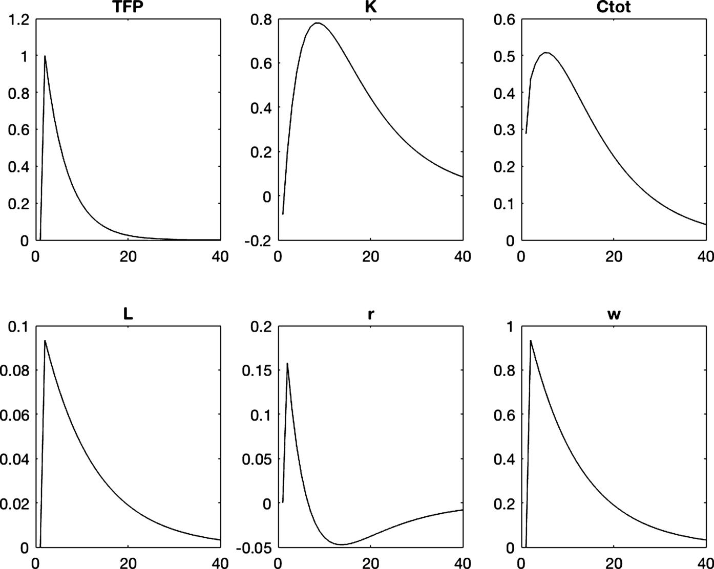
Computing the amount of extra insurance provided by the truncation. The structure of the truncation provides an additional transfer to any agents, summarized by the amount ![]() in Eq. (21). This transfer can be seen as an extra-insurance term, as it cancels the effect of past shocks to reduce heterogeneity. As the transfer is balanced, the average value of the transfer in any period is 0. In a full-fledge Bewley model, this transfer is exactly 0 for all agents, and the whole history of idiosyncratic shock matters for each individual agent. A measure of the contribution of the transfer to any agent's income is provided by the measure
in Eq. (21). This transfer can be seen as an extra-insurance term, as it cancels the effect of past shocks to reduce heterogeneity. As the transfer is balanced, the average value of the transfer in any period is 0. In a full-fledge Bewley model, this transfer is exactly 0 for all agents, and the whole history of idiosyncratic shock matters for each individual agent. A measure of the contribution of the transfer to any agent's income is provided by the measure
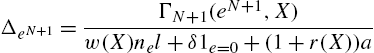
This ratio ![]() is the relative contribution of the transfer to the income of an agent having a history
is the relative contribution of the transfer to the income of an agent having a history ![]() . For the case
. For the case ![]() used in the current calibration, one finds that sd
used in the current calibration, one finds that sd![]()
![]() , which is a relatively small amount. LeGrand and Ragot (2016b) show that this standard deviation tends toward 0 as N increases. As a consequence, an increase in N reduces the amount of extra insurance provided by the truncation.
, which is a relatively small amount. LeGrand and Ragot (2016b) show that this standard deviation tends toward 0 as N increases. As a consequence, an increase in N reduces the amount of extra insurance provided by the truncation.
6 Optimal Policies
A common outcome of the previous models is that one has a finite number of types of agents to follow, as an equilibrium outcome. This allows deriving optimal policies using Ramsey techniques developed in the representative agents environments (see Sargent and Ljungqvist, 2012 for a textbook presentation), which is an interesting methodology to investigate the distortions generated by market frictions. Ragot (2016) investigates optimal monetary policy in a model with capital accumulation and flexible prices. Bilbiie and Ragot (2017) study optimal monetary policy in a monetary model with sticky-prices. Challe (2017) analyzes optimal monetary policy in a no-trade model with unemployment risk.
Recently, LeGrand and Ragot (2016b) developed a general technique to solve for optimal policies in truncated economies. They study optimal fiscal policies in a model with heterogeneous agents and aggregate shocks, with four instruments: a positive transfer, two distorting taxes on capital and labor, and public debt. This may be a promising route, as the distortions generated by incomplete insurance markets are hard to identify (see Aiyagari, 1995 and Davila et al., 2012 for a contribution about the optimality of the level of the capital stock). Nuno and Thomas (2017) solve for optimal monetary policy in a model with heterogeneous agents in continuous time, and without aggregate shocks (see also references in LeGrand and Ragot, 2016b for many relevant papers deriving optimal policies with heterogeneous agents). As far as I know, deriving optimal policies (monetary, fiscal or unemployment benefits) with incomplete markets and aggregate shocks is only easily done in a reduced-heterogeneity equilibrium, whereas it is impossible at this stage in full-fledged incomplete-market models.
7 Comparison with Other Approach Using Perturbation Methods
It maybe useful to compare the methods presented in this chapter with other methods using perturbation techniques. The key similarity of methods of this chapter is indeed to use perturbation methods around a steady state with idiosyncratic risk but with a finite state-space support as an equilibrium outcome. In addition, the state space for the aggregate risk has a continuous support, as in the DSGE literature. The model can be simulated with a finite number of equations using perturbations and software as DYNARE can be used.
Other strategies have been used to make possible the use perturbation methods.5 First, Reiter (2009) uses perturbation methods to solve for aggregate dynamics around a steady-state equilibrium of a Bewley model, with idiosyncratic shock but no aggregate shock. These techniques, used for instance in McKay and Reis (2016b), linearize policy rules around an equilibrium distribution, which has an infinite support (but the aggregate state has a finite support).
Mertens and Judd (2012) use perturbation methods around a steady-state with neither aggregate nor idiosyncratic shock. They use a penalty function to pin down steady-state portfolios (which are not determined without risks). Other papers using perturbation method but restricting exogenously the state-space are Preston and Roca (2007) and Kim et al. (2010). For instance, one can solve the model using an exogenous finite grid for the saving decisions.
The techniques presented in this chapter implied that the reduction in heterogeneity appears has an equilibrium outcome. To summarize the previous remarks, the gain is threefold.
First, this allows to consider many assets. For instance, Challe et al. (2013) price arbitrarily large number of maturities of the yield curve. LeGrand and Ragot (2016a) price both assets and derivative assets in the same model. This last two papers consider a finite state space for the aggregate risk. Considering different assets, some recent contributions in households finance show that non-convex portfolio adjustment costs (such as fixed costs) are necessary to rationalize households reaction to fiscal stimulus. This is the outcome of the recent literature on wealthy hand-to-mouth agents (Kaplan et al., 2016 and Ragot, 2014). The ability of reduced heterogeneity models to reproduce the data with such costs is an open question. Indeed, participation decision would depends on idiosyncratic histories, but they would have not to change with aggregate shocks.
Second, having a finite number of equations (in a possibly large model) allows using econometric techniques, such as Bayesian estimation, which are then relatively easy to implement. This is done in Challe et al. (2017) to quantify the contribution of precautionary saving to the business cycle in the US.
Third, the finite number of equations permits the derivation of optimal policies in these environments. This last properties allow considering rich and relevant tradeoffs for both fiscal and monetary policies, about redistribution, insurance, and incentives.
The cost of using the models presented in this chapter is that the representation of inequality is simplified in all cases compared to full-fledged Bewley models. As a consequence, these models are less useful when one wants to describe in details inequalities generated by self-insurance for uninsurable risks. Nevertheless, models with truncation in the space of idiosyncratic histories can generate an arbitrarily high number of agents to match any targeted wealth distribution. As a consequence, this type of model is more suited for quantitative work focusing cross-sectional heterogeneity.
8 Heterogeneous Expectations
The previous models have been presented under the assumption that agents share the same information set and form rational expectations. The gain of this assumption is that expectations are consistent with the model, what is an appealing property, and that they are the same for all agents. This last outcome is not totally consistent with data surveys, which shows heterogeneity in expectation about aggregate variables (see Carroll, 2003; Branch, 2004; and Massaro, 2013) and heterogeneity in expectation formation for the same information set (see Hommes, 2011 and Coibion and Gorodnichenko, 2015). A second line of research, called Agent-Based Modeling (ABM) departs from rational expectations in assuming that agents follow simple rules, and change rules according to interactions, or that they use expectations formation rules that differ from rational expectations. Hommes (2006) and LeBaron (2006) provide early surveys of this literature; Branch and McGough (2018) and Dieci and He (2018) give up to date state of the art surveys of heterogeneous expectations models in macroeconomics and finance respectively. The frontier between these two lines of research (rational and non-rational expectations) is still visible in the reference lists of various papers, but it can be expected to disappear progressively, as a growing literature investigates relevant models of expectation formation.
The tools developed in this chapter could be useful to model heterogeneous expectations in a tractable way, and thus contribute to close the gap between these two literatures. First, in some models agents choose in each periods the rules to form expectations (Branch and McGough, 2009; Massaro, 2013) or how much effort to invest to form expectation, as in the rational inattention literature (see Andrade and Le Bihan, 2013; or Vellekoop and Wiederholt, 2017 and the references in this paper). As the various equilibrium structures presented in the previous sections don't depend on rational expectations to reduce heterogeneity, they could be useful to construct models with a finite number of different expectations. Models where expectations are a state variable, as in learning models, may also be consistent with previous models. For instance, if agents experiencing the same history of shocks for a long period of time converge to the same expectations, then a truncation in histories of idiosyncratic shocks could also be a satisfactory assumption. Finally, as noted by Den Haan (2014) the case where some agents form rational expectations whereas others are boundedly rational are difficult to solve. The models presented here could allow to reduce heterogeneity among rational agents and could help to solve some of those models.
9 Concluding Remarks
This chapter surveys a class of heterogeneous-agent models, where heterogeneity is finite as an equilibrium outcome. Agents differ according to “shocks” defined in a broad sense that occur in their life. We focused more precisely on representations of reduced heterogeneity with rational expectations which can be solved with perturbation methods for the aggregate shocks. This allows introducing many other “frictions” studied in the literature, such as search-and-matching in the labor market, sticky prices, heterogeneity in skills, habit formation, and son on. These models can be estimated, using a vast information set, including times-series and cross-sectional information. Integrated models with both uninsurable shocks, a role for forward-looking behavior together with relevant heterogeneous expectations would be a good laboratory to quantify the relative importance of these various ingredients.
Finally, the models of this chapter has focused on households heterogeneity, leaving aside other forms of heterogeneity among firms or financial intermediaries. This opens a deeper question about the relevant level of aggregation to think about heterogeneity, and which type of heterogeneity matters for economic analysis. If a recent consensus seems to emerge about the importance of households heterogeneity, the interactions of various types of heterogeneity seem an interesting line of research.