
Heterogeneous Expectations and Micro-Foundations in Macroeconomics✶
William A. Branch⁎,1; Bruce McGough† ⁎University of California, Irvine, CA, United States
†University of Oregon, Eugene, OR, United States
1Corresponding author. email address: [email protected]
Abstract
This chapter provides an overview of recent models of heterogeneous expectations in macroeconomics. We begin with a description of household behavior in an environment with features common to many models in asset pricing, monetary theory, and New Keynesian macroeconomics. We demonstrate issues facing modelers when agents are boundedly rational and have (possibly) heterogeneous beliefs about the future evolution of endogenous state variables. These issues can be summed up in three broad categories: boundedly rational decision making, aggregation of decision rules, and the appropriate equilibrium concept. After having laid out the basic underlying theories we present several applications that illustrate the non-trivial implications of heterogeneous expectations for economic outcomes. Our applications include asset-pricing and bubbles, trading inefficiencies in monetary economies, and monetary policy design.
Keywords
Heterogeneous expectations; DSGE models; Bounded rationality; Asset pricing; Monetary theory; Monetary policy
1 Introduction
Modern macroeconomic models are built on micro-foundations: households and firms are dynamic optimizers in uncertain environments who interact in markets that clear in general equilibrium. Because decision-making is intertemporal, and the future is uncertain, macroeconomic models impart an important role to households' and firms' expectations about future states of the economy. Despite the importance of expectations, the benchmark approach is to assume homogeneous rational expectations, where all agents in the economy hold similar and correct views about the dynamic evolution of economic variables. Even in models of adaptive learning, e.g. Evans and Honkapohja (2001), individuals and firms are typically assumed to forecast using the same econometric model.
Nevertheless, there is substantial empirical and experimental evidence that individuals and firms have heterogeneous expectations. For example, Fig. 1 plots the interquartile range from individual inflation probability forecasts published by the Survey of Professional Forecasters (SPF) over the period 1992.1–2010.4. The IQR gives a good measure of the range of views in the SPF. The left plot is the histogram of the IQR in the sample, while the right plot is the time-series of the median IQR in each quarterly survey. Evidently, there is substantial heterogeneity among professional forecasters and, importantly, the degree of heterogeneity evolves over time.
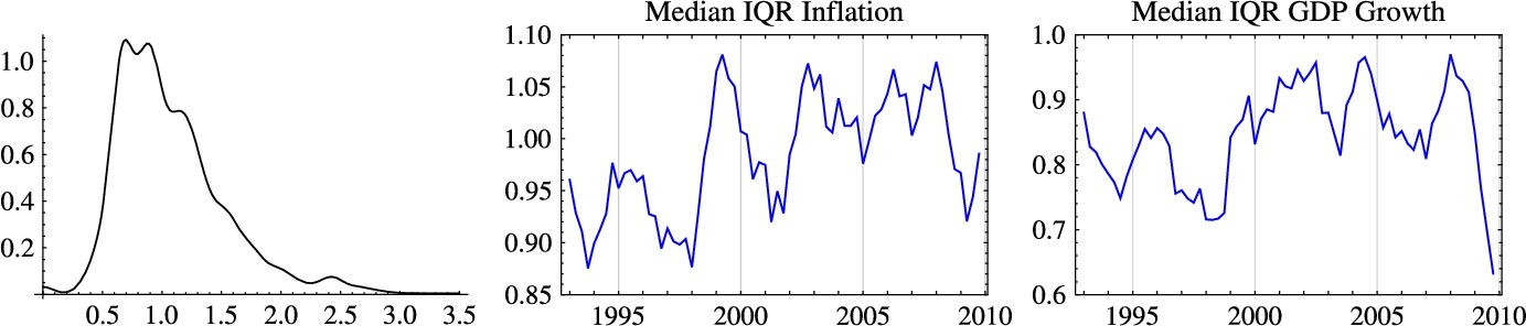
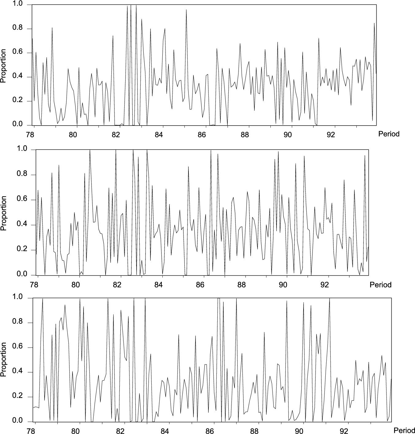
Fig. 2 plots an estimated time-series of likely forecasting methods used by respondents in the Michigan Survey of Consumers' inflation expectation series. This figure comes from Branch (2004) who estimates a model of expectation formation where households select from a set of standard statistical forecasting models, each differing in complexity and parsimony, in such a way that people favor predictors with lower forecast errors net of complexity costs. In this figure, and a substantial body of other research, there is strong evidence of time-varying expectational heterogeneity. Finally, in a series of learning-to-forecast experiments, Hommes (2013) shows strong evidence of heterogeneous expectations even in simple, controlled laboratory environments.1
A burgeoning literature studies the implications of heterogeneous expectations for dynamic, stochastic, general equilibrium (DSGE) models. This literature, motivated by these empirical facts, introduce agents with different beliefs into micro-founded models. This step of bringing bounded rationality into models with micro-foundations brings certain challenges to modelers. In particular, we begin with a discussion of the following three key questions about how to model heterogeneous beliefs in DSGE models:
- 1. How to model individual behavior given the available forecasting models?
- 2. Given a distribution of individuals across forecasting models, how are endogenous variables determined?
- 3. How are individuals distributed across forecasting models?
To address these questions we adopt a stylized DSGE environment that nests benchmark models in monetary theory, asset-pricing, and New Keynesian business cycles. The framework, which is outlined in Section 2.2, is a simplified version of Rocheteau and Wright (2011) which combines the New Monetarist monetary model with search frictions by Lagos and Wright (2005) with a Lucas asset-pricing model. By turning the search frictions off, the model reduces to a standard asset-pricing model. If we set the dividend flow to zero, the model is isomorphic to a pure monetary economy. This simple framework is able to demonstrate many of the important implications of heterogeneous expectations for the macroeconomy and asset-pricing.
We then turn to address the first question, namely, how to model the decision making of boundedly rational agents. A substantial segment of the literature follows a reduced-form approach, where the conditional expectations in the equations derived under rational expectations are replaced with a convex combination of heterogeneous expectations operators. More recently, the frontier of the adaptive learning literature adopts an “agent-level” approach that takes as given a set of behavioral primitives for individual decision-making. These behavioral primitives are based on two observations. First, agents who make boundedly rational forecasts may also make boundedly optimal decisions. Second, aggregation into equilibrium equations should follow a temporary equilibrium approach where aggregation occurs after imposing boundedly rational decision-making. The literature has proposed a variety of behavioral primitives, some based on anticipated utility maximization and others based on internal rationality. In Section 2.3 we review these approaches while discussing strengths and drawbacks of each alternative.
The link between individual decisions and aggregate outcomes is provided by temporary equilibrium: individual-level decision rules and the distribution of agents across forecasting rules are coordinated through market clearing. With properly specified forecasting rules, this leads to a temporary equilibrium law of motion that can be written entirely in terms of aggregate state variables. Section 2.4 briefly discusses this analysis in the context of our simple environment, and also discusses some potential impediments.
Our analysis is complete by specifying how the distribution of agents across forecasting models is determined as an equilibrium object. Most of the literature follows the seminal Brock and Hommes (1997) by modeling expectation formation as agents rationally choosing a predictor from a finite set of forecasting models. That is, expectation formation is a discrete choice in a random utility setting, where the distribution of agents across models is given by a multinomial logit (MNL) mapping. There have been two ways in which agents might not have rational expectations and select heterogeneous predictors. The first, called rationally heterogeneous expectations, is when rational expectations is available to agents, as well as other predictors such as adaptive and naive expectations, but they must pay a higher cost to do so. This cost is meant to proxy for computational and cognitive costs in forming rational expectations. If the utility associated with predictor choice is subject to an idiosyncratic preference shock, then heterogeneous beliefs can arise as an equilibrium object of the model. The second approach, based on Branch and Evans (2006), rules out that agents are able to form rational expectations and instead they must select from a set of parsimonious forecasting models. Branch and Evans (2006) define a Misspecification Equilibrium as occurring when individuals only select the best performing models from a restricted set.2 Of course, which models are best performing is an equilibrium property and we demonstrate a variety of environments where Intrinsic Heterogeneity can arise.
Having laid out the key theoretical issues with incorporating, and deriving, heterogeneous expectations, the rest of the chapter focuses on applications. Section 4 focuses on asset-pricing applications. Here we show that asset-pricing models with heterogeneous expectations are able to explain key empirical regularities such as bubbles/crashes, regime-switching returns and volatilities, and excess volatility. We then, in Section 5, turn to a pure monetary economy and show how heterogeneous beliefs can alter the nature of trade in economies with over-the-counter frictions. An important result here is that trading between agents with heterogeneous beliefs must also specify higher-order beliefs and these may lead to a failure for buyers and sellers to successfully execute a trade. That is, there can be an extensive margin of trade that arises from heterogeneous expectations. However, these higher order beliefs also induce people to make more cautious offers, hoping to avoid times when their offers are rejected, and so affect the intensive margin of trade as well. We show that heterogeneous expectations can have important welfare implications and can also explain puzzling experimental results.
We then extend the basic framework to the New Keynesian model. Here we show how a basic property of heterogeneous expectations models, “stability reversal,” can have important implications for the design of monetary policy. A general principle of heterogeneous expectations is the tension between forward-looking rational expectations and backward-looking adaptive expectations and learning models. Homogeneous rational expectations models that are determinate (dynamically unstable) can be indeterminate (dynamically stable) with homogeneous adaptive expectations: adaptive beliefs can reverse the stability properties of rational expectations models. Thus, there is a tension between the repelling and attracting forces inherent to heterogeneous expectations. Brock and Hommes (1997) demonstrated, with masterful force, how these attracting/repelling forces can lead to periodic and complex dynamics. An important factor for the existence of complex belief dynamics is the self-referential property of the model, and, in New Keynesian models the policy rule followed by the central bank can alter the strength of expectational feedback. We demonstrate how a policy designed to adhere to the Taylor principle under rational expectations can destabilize an economy with even just a small amount of steady-state equilibrium fraction of adaptive agents. We also show that policy rules can affect that steady-state equilibrium fraction and potentially lead to hysteresis effects for plausibly strong inflation reaction coefficients in Taylor-type rules. Finally, we show how heterogeneous expectations can lead to multiple stable equilibria including the possibility of recurring collapses to a (stable under learning) liquidity trap.
This chapter proceeds as follows. Section 2 defines the notion of an expectations operator, introduces the model, and discusses the micro-foundations and aggregation of heterogeneous beliefs. Section 3 introduces the two types of equilibria considered in this chapter: rationally heterogeneous expectations and misspecification equilibria. The stability reversal principle is introduced in this section. Section 4 presents applications to asset-pricing models, while Section 5 focuses on pure monetary economies. Section 6 presents results for DSGE models.
2 Expectations Operators and Bounded Rationality
In macroeconomic models, economic agents make decisions in dynamic, uncertain environments and, thereby, confront two related, but conceptually distinct, issues: how to make forecasts given the available information; and, how to make decisions given the available forecasts. The rational expectations hypothesis joins these two aspects of agent-level behavior through the cross-equation restrictions imposed by the equilibrium, i.e. optimal forecasts depend on actions and optimal actions depend on forecasts. This chapter focuses on bounded rationality and heterogeneous expectations, an environment where the strict nature of the link is broken, and the agents' forecasting and decision-making problems may be treated separately. Before discussing the forecasting problem, the ways in which heterogeneous beliefs can arise in equilibrium, and the resulting applications, we begin with a review of boundedly rational decision-making.
In order to motivate an equilibrium with heterogeneous expectations, we follow the adaptive learning literature that has recently turned towards a more careful modeling of the decision-making process made by individuals given that forecasts are not fully rational. This “agent-level approach” is distinguished from reduced-form learning – where the conditional expectations in the equilibrium equations derived under rational expectations are replaced with a heterogeneous expectations operator – in two important ways: first, it is reasonable to assume that agents who make boundedly rational forecasts may also make boundedly optimal decisions; and second, aggregation into equilibrium equations should take place after boundedly-rational behavior has been imposed. The first point, the possibility of boundedly optimal decision-making, requires that we take a stand on – i.e. specify behavioral primitives governing – how agents make decisions given their forecasts; and the second point, concerning the aggregation of boundedly rational behavior, demands a temporary equilibrium approach. This section reviews several approaches pursued in the literature and shows how to aggregate the agent-level decision rules.
2.1 Expectations Operators
The literature on heterogeneous expectation formation is influenced, in part, by the adaptive learning literature (e.g. Evans and Honkapohja, 2001). In this class of models, fully rational expectations are replaced by linear forecasting rules with parameters that are updated by recursive least squares. In this chapter, we imagine different sets of agents who engage in economic forecasting while recognizing there may exist heterogeneity in forecasting rules. Some examples of heterogeneity consistent with our framework include the following: some agents may be rational while others adaptive, as has been examined in a cobweb model by Brock and Hommes (1997) and found empirically relevant in the data in Branch (2004); agents may have different information sets (e.g. Branch, 2007); or, they may use structurally different learning rules as in Honkapohja and Mitra (2006). Our goal is to extend this notion of agents as forecasters to the agents' primitive problem, and to characterize a set of admissible beliefs that facilitates aggregation.
Denote by ˆEτt![]() a (subjective) expectations operator; that is, ˆEτt(xt+k)
a (subjective) expectations operator; that is, ˆEτt(xt+k)![]() is the time t expectation of xt+k
is the time t expectation of xt+k![]() formed by an agent of type τ. We require that
formed by an agent of type τ. We require that
- A1. Expectations operators fix observables.
- A2. If x is a variable forecasted by agents and has steady state ˉx
 then ˆEτˉx=ˉx
 .
. - A3. If x, y, x+y
 and αx are variables forecasted by agents then ˆEτt(x+y)=ˆEτt(x)+ˆEτt(y)
 and ˆEτt(αx)=αˆEτt(x)
 .
. - A4. If for all k≥0
 , xt+k
 and ∑kβt+kxt+k
 are forecasted by agents then
ˆEτt(∑k≥0βt+kxt+k)=∑k≥0βt+kˆEτt(xt+k).

- A5. ˆEτt
 satisfies the law of iterated expectations (L.I.E.): If x is a variable forecasted by agents at time t and time t+k
 then ˆEτt∘ˆEτt+k(x)=ˆEτt(x)
 .
.
These assumptions impose regularity conditions consistent with the literature on bounded rationality and they facilitate aggregation in a linear, or linearized environment. Assumption A1 is consistent with reasonable specifications of agent behavior (the forecast of a known quantity should be the known quantity). Assumption A2 requires some continuity in beliefs in the sense that, in a steady state, agents' beliefs will coincide. Assumptions A3 and A4 require expectations to possess some linearity properties. Essentially, linear expectations require agents to incorporate some economic structure into their forecasting model rather than, say, mechanically applying a lag operator to every random variable.
Assumptions A5 restricts agents' expectations so that they satisfy the law of iterated expectations at an individual level. The L.I.E. at the individual level is a reasonable and intuitive assumption: agents should not expect to systematically alter their expectations. In deriving the New Keynesian IS curve, with heterogeneous expectations, Branch and McGough (2009) imposed an additional assumption of the L.I.E. at the aggregate level, essentially ruling out higher order beliefs. In other applications, such as the New Monetarist search model, we explicitly model higher-order beliefs by assuming that an expectation operator consists of two components, a point estimate given by Eτt![]() and an uncertainty measure Fτt(⋅,Σ)
and an uncertainty measure Fτt(⋅,Σ)![]() .
.
2.2 The Economic Environment
Before turning to a discussion of bounded optimality and aggregation of heterogeneous expectations, it is useful to describe a general economic environment that forms the basis for many of the applications in this chapter. The environment is based on a Lucas (1978) asset-pricing model with consumption risk in the form of a frictional goods market characterized by bilateral trading and a limited commitment problem. By opening and closing the frictional market we are able to nest a standard asset-pricing model or a search-based New Monetarist type model, depending on the desired application. We turn to a brief description of the environment, and then develop the analysis as the chapter progresses.
Time is discrete, and each time period is divided into two sub-periods. There are two types of non-storable goods: specialized goods, denoted q, that are produced and consumed in a market that opens during the first sub-period (“DM”); and general goods, denoted x, that are produced and consumed in a competitive market (“CM”) during the second sub-period. There are two types of agents: “buyers” and “sellers”. All agents produce the general good using the same technology that is linear in labor. We assume that labor is traded in the competitive market at a real wage of wt![]() , which, in equilibrium, will equal the real wage in terms of the numeraire good. When we develop results for a standard Lucas asset-pricing model, we assume a perfectly inelastic labor supply so that the model reduces, essentially, to an endowment economy. Thus, the competitive market represents the part of the environment that is standard in macro DSGE models like the New Keynesian model or the Lucas asset-pricing model. In the specialized goods market, though, buyers can consume but not produce the specialized good while sellers can produce but cannot consume. Moreover, trade in these markets is characterized by a limited commitment friction where buyers are unable to commit to repay unsecured debt using their proceeds from producing in the competitive market. Thus, this part of the model captures environments with frictional goods markets where assets such as fiat money, stocks or bonds are used as payment instruments. Some of the most interesting, and recent, applications of heterogeneous expectations occur in such markets. We assume that with probability σ buyers will have preferences for the specialized goods. By setting σ=0
, which, in equilibrium, will equal the real wage in terms of the numeraire good. When we develop results for a standard Lucas asset-pricing model, we assume a perfectly inelastic labor supply so that the model reduces, essentially, to an endowment economy. Thus, the competitive market represents the part of the environment that is standard in macro DSGE models like the New Keynesian model or the Lucas asset-pricing model. In the specialized goods market, though, buyers can consume but not produce the specialized good while sellers can produce but cannot consume. Moreover, trade in these markets is characterized by a limited commitment friction where buyers are unable to commit to repay unsecured debt using their proceeds from producing in the competitive market. Thus, this part of the model captures environments with frictional goods markets where assets such as fiat money, stocks or bonds are used as payment instruments. Some of the most interesting, and recent, applications of heterogeneous expectations occur in such markets. We assume that with probability σ buyers will have preferences for the specialized goods. By setting σ=0![]() , the economic environment collapses into a standard environment without any real frictions.
, the economic environment collapses into a standard environment without any real frictions.
There exists a single storable good, an asset a that yields a stochastic payoff yt![]() . This asset could be fiat money, with yt=0
. This asset could be fiat money, with yt=0![]() , a Lucas tree with a stochastic dividend, or a risk-free bond with a known payoff. Depending on the frictions in the specialized goods market, the asset can be used to smooth consumption or as a liquid asset used in quid pro quo trade in the specialized goods market. That is, the frictional goods market gives a precautionary savings motive to hold the asset to insure against random consumption opportunities for the specialized good. Assume that households have separable preferences over the general good, the specialized good, and leisure.
, a Lucas tree with a stochastic dividend, or a risk-free bond with a known payoff. Depending on the frictions in the specialized goods market, the asset can be used to smooth consumption or as a liquid asset used in quid pro quo trade in the specialized goods market. That is, the frictional goods market gives a precautionary savings motive to hold the asset to insure against random consumption opportunities for the specialized good. Assume that households have separable preferences over the general good, the specialized good, and leisure.
2.3 Bounded Optimality
We now turn to agent-level decision-making taking the expectations operators as given. To best illustrate the ideas reviewed here, we develop them within the context of a very simple asset-pricing model. We, therefore, take the economic environment described above and shut-down the frictional goods market.
2.3.1 Rational Expectations
Assume that there is a fixed quantity (unit mass) of the asset (Lucas trees) each of which yields per-period non-storable stochastic dividend yt=y+εt![]() , where εt
, where εt![]() is zero mean, i.i.d. and has small support (so that yt>0
is zero mean, i.i.d. and has small support (so that yt>0![]() ). Each agent is initially endowed with a unit of assets, discounts the future at rate β, and receives per-period utility from consuming the dividend, as measured by the function u. Note that agents are assumed identical, except possibly in the way they form forecasts and make decisions.
). Each agent is initially endowed with a unit of assets, discounts the future at rate β, and receives per-period utility from consuming the dividend, as measured by the function u. Note that agents are assumed identical, except possibly in the way they form forecasts and make decisions.
Under the rational expectations hypothesis (REH), it is sufficient to consider the behavior of a representative agent. This agent solves the following problem:
(1) maxat+1≥0E∑t≥0u(ct)ptat+1=(pt+yt)at−ct,

where at![]() is the quantity of the asset held at the beginning of time t, ct
is the quantity of the asset held at the beginning of time t, ct![]() is consumption in time t, and pt
is consumption in time t, and pt![]() is the asset's (ex dividend) price in time t in terms of consumption goods.
is the asset's (ex dividend) price in time t in terms of consumption goods.
Because in a rational expectations equilibrium agents are identical, ct=yt![]() , the representative agent's Euler equation must be satisfied:
, the representative agent's Euler equation must be satisfied:
u′(yt)=βEt(pt+1+yt+1pt)u′(yt+1).
Thus the non-stochastic steady state of this model (or the perfect-foresight REE in case income is non-stochastic) is given by
(2) p=(β1−β)y,
which is the present value of the expected dividend flow.
The analysis of the model under the REH is quite straightforward from a modeler's perspective, but agents themselves are unrealistically sophisticated: they are assumed to know the endogenous distribution of pt![]() , fully solve their dynamic programming problem given this knowledge, and further, this knowledge must be common among agents.
, fully solve their dynamic programming problem given this knowledge, and further, this knowledge must be common among agents.
In the following subsections we provide various models of decision-making that do not require these assumptions. Once departing from the rational expectations hypothesis, the modeler is confronted with whether to require that boundedly rational agents take the evolution of their beliefs as a constraint on their decision-making. Or, should they satisfy behavioral primitives that (mistakenly) take their beliefs as having come from a completed learning process? The latter approach – called the anticipated utility approach – is the benchmark in the literature and forms the basis for the discussion in the next several sections. Below, we discuss alternative implementations of the anticipated utility approach as well as some of the associated drawbacks.
2.3.2 The Shadow-Price Approach
The first approach to boundedly rational decision making that we consider is shadow price learning, developed by Evans et al. (2016) as a general approach to boundedly-optimal decision making. We now relax the representative agent assumption and consider agents who are identical except for expectations, indexed by type-j. Shadow-price learning is based on two simple assumptions: agents make linear forecasts and make decisions by contemplating trade-offs as measured by shadow prices.
Within the context of the current asset-pricing model, let λjt![]() be the perceived time-t value of an additional unit of the asset for an agent of expectations-type j. To make a time t consumption decision, the agent employs a variational thought experiment about the savings/consumption tradeoff: by reducing consumption by one unit today and increasing asset holdings tomorrow by 1/pt
be the perceived time-t value of an additional unit of the asset for an agent of expectations-type j. To make a time t consumption decision, the agent employs a variational thought experiment about the savings/consumption tradeoff: by reducing consumption by one unit today and increasing asset holdings tomorrow by 1/pt![]() an agent will equate
an agent will equate
(3) u′(cjt)=βptˆEjtλjt+1.

To determine consumption, the modeler must take a stand on how ˆEjtλjt+1![]() is formed, as well as a forecasting rule for pt
is formed, as well as a forecasting rule for pt![]() . Given a specification for the forecasting models, the modeler can solve for the consumption rule by combining the budget constraint (1) and Eq. (3). Plugging the consumption rule into the budget constraint determines the agent's asset demand as a function of price, dividend, asset holdings and beliefs:
. Given a specification for the forecasting models, the modeler can solve for the consumption rule by combining the budget constraint (1) and Eq. (3). Plugging the consumption rule into the budget constraint determines the agent's asset demand as a function of price, dividend, asset holdings and beliefs:
(4) ajt+1=aSP(pt,yt,ajt,ˆEjtλjt+1).
In the literature, and the examples presented below, boundedly rational beliefs are typically modeled as functions of past data. To update beliefs over time as new data become available some proxy data for λt![]() must be computed, and for this the agent again employs another variational thought experiment: given the consumption choice, the benefit from an additional unit of the state today is
must be computed, and for this the agent again employs another variational thought experiment: given the consumption choice, the benefit from an additional unit of the state today is
(5) λjt=(pt+yt)u′(cjt).
More generally, the envelope condition provides a way to compute the observed value for the shadow price. Thus, the shadow price approach provides a set of behavioral primitives consistent with optimization but does not require the full sophistication required of the agent in order to solve the complete dynamic programming problem.
2.3.3 The Shadow-Price Approach in the Linearized Model
A particularly nice feature of the shadow price approach is that it is easily employed in non-linear environments: no linearization was needed to determine demand (4). Further, note that this approach is amenable to any expectations operator satisfying the axioms (and based on linear forecasting models).3 Most other implementations of boundedly-rational decision-making are developed in a linearized environment, and for comparison purposes, we consider a linearized version of shadow-price learning here.
Log-linearizing (3) and (5) around the non-stochastic steady state (2) (and using c=y![]() , which follows from the axioms) provides
, which follows from the axioms) provides
(6) cjt=υ−1(pt−ˆEjtλjt+1)λjt=−υcjt+βpt+βyyt,
where now all variables are written in proportional deviation from steady state form, and υ=−cu″(c)/u′(c)![]() . Eq. (6) is consistent with general expectations operators, but as above, it is standard to cast Ejtλjt+1
. Eq. (6) is consistent with general expectations operators, but as above, it is standard to cast Ejtλjt+1![]() as a linear function of state variables. These equations can be coupled with the linearized budget constraint to compute the linearized asset demand equation
as a linear function of state variables. These equations can be coupled with the linearized budget constraint to compute the linearized asset demand equation
(7) ajt+1=aSPlin(pt,yt,ajt,ˆEjtλjt+1).
As long as beliefs are linear functions of prices and dividends, then asset-demand is a function only of state variables. Importantly, aSPlin![]() is linear, which allows for tractable equilibrium analysis.
is linear, which allows for tractable equilibrium analysis.
2.3.4 The Euler Equation Approach in the Linearized Model
Under shadow-price learning, the behavioral primitive is that agents make decisions based on tradeoffs measured by shadow prices. Here we take a different perspective, Euler-equation learning as advanced by Honkapohja et al. (2013): agents make decisions based on their perceived Euler equation. We continue to work within the linearized model.
The linearized Euler equation is given by
(8) cjt=υ−1pt+ˆEjtcjt+1−βυ−1ˆEjtpt+1−βyυ−1ˆEjtyt+1.
Note that (8) identifies the agent's decision in terms of a general expectations operator, but as in the shadow-price approach, it is common to assume agents use linear forecasting models to form expectations; however, rather than their shadow-value this time agents are required to forecast their own consumption plan. Coupled with the linearized budget constraint and perceived Euler equation, we can compute asset demand:
(9) ajt+1=aELlin(pt,yt,ajt,ˆEjtcjt+1,ˆEjtpt+1),
which, as before, depends on beliefs, and is linear in prices. As before, provided that beliefs are linear functions of prices and dividends, the demand function can be written entirely in terms of state variables.
2.3.5 The Finite Horizon Approach in the Linearized Model
The shadow price and Euler equation approaches, as developed above, are based on one-step-ahead forecasts. When longer planning horizons are relevant, e.g. in case of anticipated structural change, a modification is in order. In this section we consider the implementation developed in Branch et al. (2012). The idea is simple: agents forecast their terminal asset position to solve their N-period consumption-savings problem. This finite-horizon learning approach places forecaster – who typically forecasts over a finite horizon – on equal footing with decision-makers.
While the model remains the same, it is convenient to change notation. First, go back to levels. Let ˆat=pt−1at![]() be the goods-value of the asset held at time t and let Rt=p−1t−1(pt+yt)
be the goods-value of the asset held at time t and let Rt=p−1t−1(pt+yt)![]() be the return. The flow constraint may be written
be the return. The flow constraint may be written
cjt=Rtˆajt−ˆajt+1.
Now let Dt+k=∏kn=1R−1t+n![]() , with Dt=1
, with Dt=1![]() , be the cumulative discount factor. The N-period budget constraint is then given by
, be the cumulative discount factor. The N-period budget constraint is then given by
(10) N∑k=0Dt+kct+k=Rtˆat−Dt+Nˆat+N+1.

In differential form, we have
yN∑k=1dDt+k+N∑k=0βkdcjt+k=ˆadRt+β−1dajt−βNdajt+N+1−ˆadDt+N,
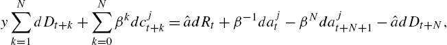
where we have used that in steady state, y=c![]() and R=β−1
and R=β−1![]() . Simplifying, using that dDt+k=−βk+1∑kn=1dRt+n
. Simplifying, using that dDt+k=−βk+1∑kn=1dRt+n![]() and returning to log-deviation form, we arrive at
and returning to log-deviation form, we arrive at
(11) yN∑k=0βkcjt+k=ˆaβ−1Rt+β−1ˆaˆajt−βNˆaˆajt+N+1+ˆaβNk∑n=1Rt+k+yN∑k=1βkk∑n=1Rt+n,
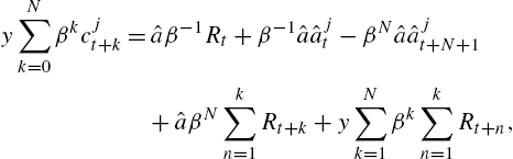
which is the agent's linearized budget constraint with planning horizon N.
The linearized Euler equation yields
(12) ˆEjtcjt+k=cjt+υ−1k∑n=1ˆEjtRt+n.
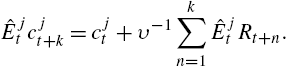
Taking expectations of (11) (relying on the axioms), and using (12) to eliminate ˆEjtcjt+k![]() , we may write current consumption as linear in ajt,Rt,ˆEjtajt+N+1
, we may write current consumption as linear in ajt,Rt,ˆEjtajt+N+1![]() , and ˆEjtRt+n
, and ˆEjtRt+n![]() , for n=1,…,N
, for n=1,…,N![]() . By providing the agent with linear forecasting models for asset holdings and returns, the current consumption and savings decisions may be determined in terms of beliefs and observable state variables.
. By providing the agent with linear forecasting models for asset holdings and returns, the current consumption and savings decisions may be determined in terms of beliefs and observable state variables.
2.3.6 The Infinite Horizon Approach in the Linearized Model
Letting the planning horizon N go to infinity and imposing the transversality condition provides the infinite horizon approach. Eq. (11) becomes the usual lifetime budget constraint, which is particularly simple in our case:
(13) y∞∑k=0βkEτtcjt+k=(1−β)−1Rt+(1−β)−1ajt+y(1−β)−1∞∑k=1βkRt+k,

which, when coupled to the linearized Euler equation (12), yields
(14) cjt=y−1Rt+y−1ajt+υ−1υ∞∑k=1βkEjtRt+k.
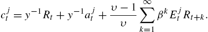
By providing the agent with linear forecasting models for returns, the current consumption and savings decisions may be determined in terms of beliefs and observables. Notice, unlike the previous approaches, with infinite-horizon learning they only need to forecast state variables beyond their own control.
The infinite horizon approach has advantages over the Euler equation in that the agents are behaving as optimizing anticipated utility maximizers. Thus, although the agents have non-rational and possibly heterogeneous expectations, they optimize given their subjective expectations. We show below that infinite horizon learning – by emphasizing decision rules that depend on expectations of state variables beyond an agent's control – can help aggregate decision rules across agents with heterogeneous expectations. From (14), the approach leads to a key result that long-run expectations play an important role in household consumption decisions. The infinite-horizon approach has been employed extensively by Preston (2005, 2006), Eusepi and Preston (2011), Woodford (2013), and recently surveyed in Eusepi and Preston (2018).
However, there are drawbacks as well. First, as a model of bounded rationality it seems unlikely that consumers hold such long-horizon expectations. Second, solving the infinite horizon problem can be technically challenging without log-linearizing the behavioral equations. While this may be appropriate in some environments such as the New Keynesian model which also is usually solved only after log-linearizing even when agents hold rational expectations, it is not a good approximation in other environments such as asset-pricing, pure monetary theory, and models with search and matching frictions. Finally, if the motivation for learning models is to place economist and economic agent on equal footing, it seems natural to model agents as finite-horizon learners who have a more limited horizon as most econometricians only forecast for so many periods into the future.
2.3.7 A Nod to Value Functions
As an alternative to the shadow-price approach, Evans et al. (2016) consider “value-function learning” within a linear-quadratic framework. Under this approach, agents estimate the value function based on a quadratic form specification and then make decisions conditional on the estimated value function. They show that asymptotic optimality obtains under the same conditions as for the shadow-price approach.
Value-function learning in the current environment is less natural: the analog to the linearized model would be to compute a second order approximation to the objective (after substituting in the non-linear budget constraint). On the other hand, the value-function approach is especially natural in discrete choice environments: Evans et al. (2016) develop a value-function learning analysis of the McCall (1970) search model where the agent must decide whether to accept an offer. They provide conditions under which a learning agent will behave optimally asymptotically.
The value function approach is also particularly convenient when special assumptions make it natural for the agent to know the value function's form. The LQ-environment considered by Evans et al. (2016) provides one framework, and the quasi-linear utility environment in many incarnations of the Lagos–Wright model provide another: Branch and McGough (2016) and Branch (2016) use precisely this approach, which is discussed below.
2.3.8 A Defense of Anticipated Utility
In models of learning and heterogeneous (non-rational) expectations, beliefs evolve over time. Households and firms solve intertemporal optimization problems that require expectations about future variables that are relevant to their decision making. Under rational expectations, an agent holds a well-specified probability distribution that, in equilibrium, is time invariant. Under learning, there is the issue of whether, and to what extent, agents explicitly account for the evolution of their beliefs when deciding on their optimal decision rules. That is, should an agent's beliefs be a state variable in their value functions?
The anticipated utility approach dictates that agents take their current beliefs as fixed when solving for their optimal plans. Given an expectation operator dated at time t, an agent is able to formulate expectations about variables relevant to their decision making over their particular planning horizon. They then solve for their optimal plan – consumption, labor hours, and asset holdings in the present environment – while assuming that their beliefs will not change in the future. As their beliefs change, they will discard their plan and formulate a new one. In a sense, an anticipated utility maximizing agent is dogmatic about their current beliefs. Conversely, a Bayesian agent would acknowledge that their beliefs evolve and treat those beliefs as a state variable with an associated law of motion. The literature on learning and heterogeneous expectations typically maintains the anticipated utility assumption for technical convenience: solving intertemporal optimization problems as a fully Bayesian agent is analytically and computationally challenging. Moreover, as we argue here the anticipated utility assumption is appealing from a bounded rationality perspective.
Cogley and Sargent (2008) directly address the inconsistency inherent to anticipated utility maximization. Each period the agent holds beliefs about all payoff-relevant variables over the planning horizon. Then when making decisions they act as if they will never change those beliefs again, that is, until the learning process has ended. In the next period they update beliefs and again pretend that they will not learn anymore. A fully Bayesian agent, however, would acknowledge their uncertainty, include their beliefs as a state variable, and assign posterior probabilities to all of the possible future paths, choosing the consumption plan that maximizes their expected utility, where expectations are taken with respect to their posterior distribution. Cogley and Sargent (2008) compare how anticipated utility consumption decisions compare to the fully Bayesian plan. They find that anticipated utility can be seen as a good approximation to fully Bayesian optimization.
This subsection briefly comments on their results, placing the discussion in the context of our present environment, and relating it to recent models of “Internal Rationality.”4 Cogley and Sargent's approach could be mapped into the present environment by assuming that the dividend growth process follows a two-state Markov chain and the agents know that the pricing function depends on the current realization of dividend growth. Cogley and Sargent's learning model imposes that the agents know that dividend growth, hence prices, follow the two-state process but they don't know the transition probabilities. Instead, they learn about these transition probabilities using past data and by updating their estimates using Bayes' rule. The Bayesian agents solve a dynamic programming problem including their beliefs about the transition probabilities in the state vector and, so, their learning rule becomes a part of the state transition equation. An anticipated utility maximizer, on the other hand, does not include the evolution of their beliefs in the state transition equation, and solves a standard dynamic programming problem assuming their beliefs are fixed.
Cogley and Sargent show that in this simple environment that the number of times that dividend growth is in a particular state is a sufficient statistic for agents' learning model. They focus on a model with finitely-lived agents. The agent considers each possible node which consists of a particular state at time t, and the number of times that it has been in a state, assigns probabilities to these nodes, and then chooses the consumption plan that maximizes expected utility. This can be done recursively using dynamic programming methods. As time advances, the number of nodes expands and the solution to the dynamic programming problem can run into the curse of dimensionality. If the agent has an infinite planning horizon, as is typical in macroeconomic and asset-pricing models, then the state space is unbounded and standard results for dynamic programming do not apply. Cogley and Sargent discuss an approximation, where since the agents are learning about an exogenous process, with no feedback from beliefs, the estimated probabilities eventually converge to their true values. So agents can take as given the value function that they will eventually converge to, and then recursively solve a finite horizon problem.
Adam et al. (2017) consider an asset-pricing model where agents are “internally rational.” Like Cogley and Sargent they expand the state vector to include agents' beliefs. However, internally rational agents do not know the pricing function and so also forecast price-growth. With a continuous Markov process for dividend growth, and other restrictions on beliefs, they are able to numerically solve for the policy function. They find that such a model can explain key asset pricing and survey data empirical regularities.
This chapter focuses on bounded rationality and heterogeneous expectations. We do not present results on internal rationality because we do not find it a realistic model of individual behavior. The motivation for heterogeneous expectations and learning models is that forming rational expectations is complex and costly. The fully Bayesian model of decision making is, in essence, a hyper-rational model of agent decision-making. Besides considering what prices and other exogenous variables might be in the future, they also take into account how their beliefs might evolve along any history of shocks. Loosely speaking, an agent who is optimistic today has to forecast how they will behave in a few years if they become pessimistic and, continuing this internal thought experiment, will they switch to being optimistic in, say, another 10 years, and so on. Given the complexity for the modeler to solve such a dynamic programming problem, the potential for the curse of dimensionality, and the possibility that standard recursive tools are not available, it strikes us as not the most compelling way to describe real-life behavior.5 The advantage of the internal rationality approach is to focus attention on the role of learning, without other assumptions about boundedly rational decision-making, and, as a benchmark like rational expectations, we agree that it is a useful theoretical approach. We are heartened that models with Euler equation learning and internal rationality produce similar asset-pricing implications.
However, the focus of this article is the extent to which bringing more realistic models of agent behavior can lead to distinct implications and provide explanations for real-world phenomena. Thus, we advocate for, and focus on, models of anticipated utility maximization.
2.4 Aggregating Household Decision Rules
Having derived the individual boundedly rational optimizing behavior of heterogeneous agents, equilibrium requires computing aggregate, or market-clearing consumption/output from which assets can then be priced. Many applications derive an aggregate asset-pricing equation that depends on the aggregate expectations operator. This section illustrates how to aggregate decision rules, while briefly discussing some challenges.
To illustrate, we adopt the Euler equation learning approach. Recall that the behavioral primitives, in the log-linearized economy, are
cjt=βRˆEjtcjt+1−βRυ−1ˆEjtRt+1cjt=ˆaR(ˆajt+Rt)−ˆaˆajt+1≡Ωjt
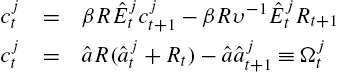
where Ωj![]() denotes (end of period) real-wealth. Iterating on the Euler equation, we have
denotes (end of period) real-wealth. Iterating on the Euler equation, we have
Ωjt=Ωj∞−βRυ−1ˆEjt∞∑k=1(βR)k−1Rt+k

where Ωj∞=limT→∞(βR)TˆEjtcT![]() . In the asset-pricing application, βR=1
. In the asset-pricing application, βR=1![]() and so the Euler equation iterated forward depends on expected limiting wealth. In a model where there is a precautionary savings motivate, for instance in the version of the model with the specialized goods market and a limited commitment friction, it is possible that R<β−1
and so the Euler equation iterated forward depends on expected limiting wealth. In a model where there is a precautionary savings motivate, for instance in the version of the model with the specialized goods market and a limited commitment friction, it is possible that R<β−1![]() and Ωj∞=0
and Ωj∞=0![]() . In this case, aggregation proceeds without any difficulty.
. In this case, aggregation proceeds without any difficulty.
When βR=1![]() , then additional assumptions on higher-order beliefs are necessary for aggregation. To illustrate this, assume that there are two expectation-types, j=1,2
, then additional assumptions on higher-order beliefs are necessary for aggregation. To illustrate this, assume that there are two expectation-types, j=1,2![]() . Then, nΩ1t+(1−n)Ω2t=(1−β)−1Rt
. Then, nΩ1t+(1−n)Ω2t=(1−β)−1Rt![]() in this linearized economy. Then
in this linearized economy. Then
(1−β)−1Rt=nΩ1t+(1−n)Ω2t=nΩ1∞+(1−n)Ω2∞−υ−1ˆEt∑k⩾1Rt+k=[1−υ−1(1−β)]ˆEtRt+1+nΩ1∞+(1−n)Ω2∞−ˆE[nΩ1∞+(1−n)Ω2∞]
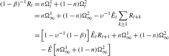
where ˆE=nˆE1+(1−n)ˆE2![]() . Thus, to have a (linearized) asset-pricing equation that depends on the aggregate expectations operator – i.e. a weighted average of heterogeneous expectations – requires that all agents agree on limiting wealth, an axiom needed for aggregation in the New Keynesian model as shown by Branch and McGough (2009). Alternatively, a model with βR<1
. Thus, to have a (linearized) asset-pricing equation that depends on the aggregate expectations operator – i.e. a weighted average of heterogeneous expectations – requires that all agents agree on limiting wealth, an axiom needed for aggregation in the New Keynesian model as shown by Branch and McGough (2009). Alternatively, a model with βR<1![]() also facilitates aggregation without difficulty.
also facilitates aggregation without difficulty.
3 Equilibria with Heterogeneous Expectations
Having developed both a general framework for non-rational expectations operators as well as a corresponding decision theory, we now turn to equilibrium considerations. There are two questions to address:
- 1. Given the distribution of agents across expectations operators, how are endogenous variables determined?
- 2. How are agents distributed across expectations operators?
The first question is straightforward to address: under the reduced form approach, a convex combination of expectations operators is imposed directly into the reduced-form expectational difference equations; while under a micro-founded approach, a temporary equilibrium is constructed by aggregating individual rules and imposing market clearing.
Three different broad mechanisms have been proposed to address the second question. Many, especially early, applications of heterogeneous expectations in macroeconomic models imposed the degree of heterogeneity exogenously, which we describe as extrinsic heterogeneity. Beginning with the seminal work by Brock and Hommes (1997), much of the literature has the distribution of agents across models as an equilibrium object. Here we review two ways in which heterogeneity can arise endogenously: first, where there is a cost to using certain types of predictors, i.e. rationally heterogeneous expectations; second, where forecasters miss-specify their models in different ways, but in equilibrium they only choose the best performing models, that is, intrinsic heterogeneity.
3.1 Extrinsic Heterogeneity
An equilibrium with extrinsic heterogeneity takes the distribution of agents across models as fixed and computes equilibrium prices and quantities. In particular, in the asset-pricing application developed in the previous section, each agent of type j, solves for their optimal consumption and asset holdings given their behavioral primitives (e.g. SP-learning, etc.), and then the temporary equilibrium pins down the price. For example, suppose J is a finite index set of types of SP-learning agents who differ only in their time-t beliefs. The asset demand of an agent of type j∈J![]() is then given by
is then given by
ajt+1=aSP(pt,yt,ajt,ˆEjtλjt+1)
Let nj![]() be the measure of type j agents. Given yt
be the measure of type j agents. Given yt![]() , beliefs {ˆEjtλjt+1}j∈J
, beliefs {ˆEjtλjt+1}j∈J![]() , and asset holdings {ajt}j∈J
, and asset holdings {ajt}j∈J![]() , the equilibrium price is determined by
, the equilibrium price is determined by
1=∑j∈Jnj⋅aSP(pt,yt,ajt,ˆEjtλjt+1)

Note that here we are using the non-linear version of SP-learning. The linearized market-clearing condition would set the sum to zero. Note also that, in this linearized case, an analytic expression for pt![]() in terms of beliefs, exogenous variables, and the distribution of asset holdings, is available.
in terms of beliefs, exogenous variables, and the distribution of asset holdings, is available.
3.2 Rationally Heterogeneous Expectations
The theory of rationally heterogeneous expectations, as formulated by Brock and Hommes (1997), holds that expectation formation is a discrete choice from a finite set of predictors.
3.2.1 Predictor Selection
In order to illustrate how the approach works in the present environment, for ease of exposition, we assume the shadow value learning formulation, and risk-neutral preferences. In this case,
(15) pt=βy+βˆEtpt+1
where ˆEt![]() is a convex combination of expectations operators:
is a convex combination of expectations operators:
ˆEtpt+1=N∑j=1njpet+1(j)
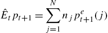
where pet+1(j)![]() is the forecast provided by predictor j, and nj
is the forecast provided by predictor j, and nj![]() is the proportion of agents using that forecast.
is the proportion of agents using that forecast.
Each individual i is assumed to select their predictor j by solving the following problem:
jt+1=argmaxj=1,...,J{Ωi(j,pet(j),pt)}
where
Ωi(j,pet,pt)=−(pt−pet(j))2−Cit(j)
The objective function Ωi![]() can be thought of as consisting of two components: −(pt−pet(j))2
can be thought of as consisting of two components: −(pt−pet(j))2![]() captures the preference for predictors that forecast well; and, Cit(j)
captures the preference for predictors that forecast well; and, Cit(j)![]() is an idiosyncratic preference shock measuring individual i's relative ease of using predictor j, i.e. it is a “cost” to using the predictor.
is an idiosyncratic preference shock measuring individual i's relative ease of using predictor j, i.e. it is a “cost” to using the predictor.
The cross-sectional distribution of the preference shock determines the distribution of agents across the predictors. We follow the discrete choice approach of Brock and Hommes (1997) and assume that Cit(j)=C(j)+ηit(j)![]() . Provided that the ηit
. Provided that the ηit![]() are i.i.d. across time and individuals and, further, have the extreme value distribution, then the fraction of individuals using predictor j, denoted nt(j)
are i.i.d. across time and individuals and, further, have the extreme value distribution, then the fraction of individuals using predictor j, denoted nt(j)![]() is given by the multinomial logit (MNL) map:
is given by the multinomial logit (MNL) map:
(16) nt(j)=nt(j,pt−1,{pet−1(τ)}Jτ=1)=exp{ω×Ω(j,pt−1,pet−1(j))}∑Nτ=1exp{ω×Ω(τ,pt−1,pet−1(τ))}

The MNL map has a long and venerable history in discrete choice decision making. It is a natural way of introducing randomness in forecasting and has a similar interpretation as mixed strategies in actions as a mechanism for remaining robust to forecast model uncertainty. The coefficient ω is referred to as the ‘intensity of choice’ and is inversely related to the variance of the idiosyncratic preference shock ηit![]() . Finite values of ω, the intensity of choice, imply less than full utility maximization. The neoclassical case is when ω→+∞
. Finite values of ω, the intensity of choice, imply less than full utility maximization. The neoclassical case is when ω→+∞![]() .
.
One note about the formulation in (16). Here nt(j)![]() is the fraction of agents holding predictor j at time t, i.e. it is the distribution at the time when markets clear and pt
is the fraction of agents holding predictor j at time t, i.e. it is the distribution at the time when markets clear and pt![]() is realized. We follow much of the adaptive learning literature in assuming a (t−1)
is realized. We follow much of the adaptive learning literature in assuming a (t−1)![]() -timing structure of information known to agents when they select predictors. Since these individuals are boundedly rational it is natural to assume that predictor choice and market outcomes are not determined simultaneously. Thus, when selecting the predictor to take into the market in time t the most recently observed data point is pt−1
-timing structure of information known to agents when they select predictors. Since these individuals are boundedly rational it is natural to assume that predictor choice and market outcomes are not determined simultaneously. Thus, when selecting the predictor to take into the market in time t the most recently observed data point is pt−1![]() .
.
3.2.2 Heterogeneous Beliefs and Economic Dynamics: Stability Reversal
Coupling predictor choice as in (16) with the pricing equation (15) can lead to interesting non-linear dynamics that exploit the mutual feedback between the pricing process – which is self-referential – and the choice of predictors. We illustrate these implications in this subsection.
Continue to assume that price is determined by (15). We will consider a simple example, as in Branch and McGough (2016), where individuals select from either a perfect foresight predictor, with a cost C>0![]() , or a simple adaptive predictor at no cost. That is, the predictors are
, or a simple adaptive predictor at no cost. That is, the predictors are
ˆE1tpt+1=pt+1ˆE2tpt+1=ˉp+θ(pt−1−ˉp)
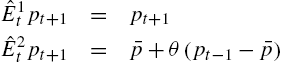
where ˉp=ˉy/(1−β)![]() is the steady-state price. Without loss of generality, set ˉy=0
is the steady-state price. Without loss of generality, set ˉy=0![]() . Then the actual law of motion is
. Then the actual law of motion is
pt=(1βnt−1)pt−1−(1−nt−1nt−1)θpt−2nt=12{tanh[ω2((pt−1−θpt−2)2−C)]+1}

Predictor selection can lead to an endogenous attracting/repelling dynamic that can lead to periodic and complex fluctuations in price. The key intuition for complex dynamics is the stability reversal property of heterogeneous expectations:
Proposition 1
Consider the case of rational versus adaptive expectations and (15) with extrinsic heterogeneity.
- a. Let n=1
 . The steady state is dynamically unstable and there exists a unique non-explosive perfect foresight equilibrium path.
 - b. Let n=0
 . The steady state is dynamically stable provided that βθ<1
 .
.
When n=1![]() , and all agents are rational, there is a unique rational expectations equilibrium that coincides with the steady-state. That is, the steady state is the only non-explosive solution to the forward expectational difference equation (15). The equilibrium is unique because the steady-state is dynamically unstable. Conversely, so long as θ is not too large – for example, 0<θ<1
, and all agents are rational, there is a unique rational expectations equilibrium that coincides with the steady-state. That is, the steady state is the only non-explosive solution to the forward expectational difference equation (15). The equilibrium is unique because the steady-state is dynamically unstable. Conversely, so long as θ is not too large – for example, 0<θ<1![]() would be sufficient – then the steady-state is dynamically stable and all paths from an initial condition on beliefs will converge to the steady-state.
would be sufficient – then the steady-state is dynamically stable and all paths from an initial condition on beliefs will converge to the steady-state.
The stability reversal property arises intuitively because perfect foresight requires forward-looking behavior and adaptive beliefs are backward-looking. This is most easily seen by noting that the expectational difference equation (15) reverses direction when, for instance, ˆEtpt+1=pt−1![]() . Therefore, forward stability implies backward stability, and vice versa. The possibility of stability reversal plays a prominent role in explaining the dynamic behavior of models with heterogeneous expectations. In subsequent sections, we present examples where stability reversal implies complex attracting/repelling dynamics.
. Therefore, forward stability implies backward stability, and vice versa. The possibility of stability reversal plays a prominent role in explaining the dynamic behavior of models with heterogeneous expectations. In subsequent sections, we present examples where stability reversal implies complex attracting/repelling dynamics.
3.3 Intrinsic Heterogeneity
In the rationally heterogeneous expectations approach, heterogeneity arises because of a cost to using a particular predictor, and for finite intensities of choice, ω, i.e. because of the idiosyncratic preference shocks. In Branch and Evans (2006) an environment is presented where heterogeneity can arise even in the neoclassical case of ω→+∞![]() . The framework developed by Branch and Evans is an extension of Brock and Hommes to a stochastic environment where agents select among a set of misspecified forecasting models. In a Misspecification Equilibrium the parameters of the forecasting models, and the distribution of agents across models, are determined jointly as equilibrium objects. Intrinsic Heterogeneity arises if agents are distributed across more than one model even as ω→∞
. The framework developed by Branch and Evans is an extension of Brock and Hommes to a stochastic environment where agents select among a set of misspecified forecasting models. In a Misspecification Equilibrium the parameters of the forecasting models, and the distribution of agents across models, are determined jointly as equilibrium objects. Intrinsic Heterogeneity arises if agents are distributed across more than one model even as ω→∞![]() . Branch and Evans (2006) developed their results within the context of a cobweb model, though Branch and Evans (2010) extend to an asset-pricing model, and Branch and Evans (2011) show existence of Intrinsic Heterogeneity in a New Keynesian model.
. Branch and Evans (2006) developed their results within the context of a cobweb model, though Branch and Evans (2010) extend to an asset-pricing model, and Branch and Evans (2011) show existence of Intrinsic Heterogeneity in a New Keynesian model.
To illustrate the approach, we extend the basic modeling environment to include two different serially correlated shocks, a dividend shock and a share-supply shock. In Branch and Evans (2010) the share-supply shock arises in an OLG model through random variations in population growth, which affects the supply of trees per person. In Branch (2016) variations in the supply can arise in the search-based asset-pricing model outlined in the previous section. Here we will illustrate the approach in the context of the search-based asset-pricing model that, with large enough liquidity services role for the asset in facilitating specialized good consumption, can feature negative feedback as in the Cobweb and New Keynesian economies.
A log-linearization to the asset-pricing equation extended to include a liquidity premium can be written as
ˆpt=α0ˆEtˆyt+1+α1ˆEtˆpt+1+α2ˆAt
for appropriately defined αk,k=0,1,2![]() .6 The stochastic process At
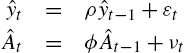
.6 The stochastic process At![]() is the supply of shares in the Lucas tree, which can be interpreted as asset float resulting from new share issuances, repurchases, and stock splits. Assume that the stochastic processes for dividends and share supply are stationary AR(1) processes, given by
is the supply of shares in the Lucas tree, which can be interpreted as asset float resulting from new share issuances, repurchases, and stock splits. Assume that the stochastic processes for dividends and share supply are stationary AR(1) processes, given by
ˆyt=ρˆyt−1+εtˆAt=ϕˆAt−1+νt
where ε,ν![]() are uncorrelated across time but are potentially correlated with each other. If there is sufficient curvature of the utility function over the specialized good then α1<0
are uncorrelated across time but are potentially correlated with each other. If there is sufficient curvature of the utility function over the specialized good then α1<0![]() and the model exhibits negative feedback. This arises when the liquidity premium is high: if the expected price of the asset is high then it will relax the liquidity constraint and individuals do not need to hold as much of the asset to facilitate specialized-goods consumption, demand for the asset goes down, and price decreases. Alternatively, for smaller liquidity premia then α1>0
and the model exhibits negative feedback. This arises when the liquidity premium is high: if the expected price of the asset is high then it will relax the liquidity constraint and individuals do not need to hold as much of the asset to facilitate specialized-goods consumption, demand for the asset goes down, and price decreases. Alternatively, for smaller liquidity premia then α1>0![]() .
.
In a rational expectations equilibrium, agents would include in their forecasting model, or perceived law of motion (PLM), both dividends and share supply. In Branch and Evans (2006), agents were assumed to select from a set of underparameterized forecasting models. In the present application, the set of forecasting models are:
ˆpt=b1ˆyt+ϵ1t⇒ˆE1tˆpt+1=b1ρˆytˆpt=b2ˆAt+ϵ2t⇒ˆE2tˆpt+1=b2ϕˆAt
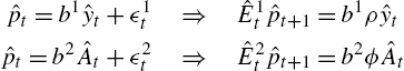
Underparameterization is motivated by real life decisions encountered by professional forecasters. Often, degrees of freedom limitations lead forecasters to adopt parsimonious models.7
Denote by n the fraction of agents who adopt the dividend-only forecasting model, i.e. “model 1”. Plugging in expectations, the actual law of motion can be written as
ˆpt=ξ0(b1,n)ˆyt+ξ1(b2,n)ˆAt
In a Misspecification Equilibrium, agents only select the best-forming statistical models. Thus, in equilibrium we require that the coefficients of the forecasting models are determined by the least-squares projection of price onto the restricted set of regressors, i.e. b1,b2![]() satisfy the least-squares orthogonality conditions
satisfy the least-squares orthogonality conditions
(17) Eˆyt(pt−b1ˆyt)=0
(18) EˆAt(pt−b2ˆAt)=0
A Restricted Perceptions Equilibrium is a stochastic process for pt![]() , given n, such that b1,b2
, given n, such that b1,b2![]() satisfy (17)–(18). In a restricted perceptions equilibrium the agents forecasting models are misspecified but, within the context of their forecasting model, they do not recognize the misspecification. A restricted perceptions equilibrium can be justified in environments where data is slow to reveal the misspecification, a property shared by most time series data.
satisfy (17)–(18). In a restricted perceptions equilibrium the agents forecasting models are misspecified but, within the context of their forecasting model, they do not recognize the misspecification. A restricted perceptions equilibrium can be justified in environments where data is slow to reveal the misspecification, a property shared by most time series data.
A Misspecification Equilibrium requires that the agents only select their best performing statistical model. Branch and Evans (2006) endogenize the distribution of agents across forecasting models, as in Brock–Hommes, by assuming they make a discrete choice and the distribution is determined by the MNL-map:
n=12{tanh[ω2F(n)]+1}≡Tω(n)
where F(n)![]() is the relative mean-squared error between predictor 1 and predictor 2 within a restricted perceptions equilibrium for a given n. Notice that the T-map: Tω:[0,1]→[0,1]
is the relative mean-squared error between predictor 1 and predictor 2 within a restricted perceptions equilibrium for a given n. Notice that the T-map: Tω:[0,1]→[0,1]![]() is continuous and so the set of equilibria is indexed by the intensity of choice ω and the properties of the function F.
is continuous and so the set of equilibria is indexed by the intensity of choice ω and the properties of the function F.
Definition 2
A Misspecification Equilibrium is a fixed point, n⁎![]() , of Tω
, of Tω![]() .
.
The set of equilibria depend on the properties of F, and can be characterized in the following way.
Proposition 3
The set of Misspecification Equilibria has one of the following properties.
- 1. If F(0)>0
 and F(1)<0
 , then as ω→∞
 , n⁎→˜n
 where F(˜n)=0
 . That is, the model exhibits Intrinsic Heterogeneity.
 - 2. If F(0)>0 and F(1)>0
 , then as ω→∞, n⁎→1
 .
. - 3. If F(0)<0
 and F(1)<0, then as ω→∞, n⁎→0
 .
. - 4. If F(0)<0 and F(1)>0, then as ω→∞, the model has multiple Misspecification equilibrium with n⁎→∈{0,˜n,1}
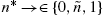 and F(˜n)=0.
Intrinsic Heterogeneity arises when agents do not want to mass on one or the other predictors, which occurs when F(0)>0,F(1)<0![]() , i.e. there is always an incentive to deviate from expectations homogeneity. In the Branch–Evans papers it was shown that Intrinsic Heterogeneity requires negative feedback, α1<0
, i.e. there is always an incentive to deviate from expectations homogeneity. In the Branch–Evans papers it was shown that Intrinsic Heterogeneity requires negative feedback, α1<0![]() , which can occur for large liquidity premia in the present environment. In the monetary policy application, negative feedback can arise when the central bank sets its policy rate according to an expectations-based Taylor-type rule with an aggressive response to expectations. Negative feedback implies that the asset pricing model features strategic substitution effects. There can also be multiple equilibria when there are sufficiently strong strategic complementarities, i.e. with α1>0
, which can occur for large liquidity premia in the present environment. In the monetary policy application, negative feedback can arise when the central bank sets its policy rate according to an expectations-based Taylor-type rule with an aggressive response to expectations. Negative feedback implies that the asset pricing model features strategic substitution effects. There can also be multiple equilibria when there are sufficiently strong strategic complementarities, i.e. with α1>0![]() . In this case, there are misspecification equilibria with all agents massed onto one model or the other, and a third misspecification equilibria that exhibits Intrinsic Heterogeneity.8
. In this case, there are misspecification equilibria with all agents massed onto one model or the other, and a third misspecification equilibria that exhibits Intrinsic Heterogeneity.8
4 Asset-Pricing Applications
Heterogeneous expectations provide a promising avenue for generating more realistic movements in asset prices than what is capable with the representative agent counterpart. This section illustrates three mechanisms for generating empirical features of asset prices. First, we present a Misspecification Equilibrium, when combined with learning, that is able to generate regime-switching returns and volatilities consistent with the data. Second, we highlight two ways in which heterogeneous expectations can lead to the endogenous emergence of bubbles and crashes.
4.1 Regime-Switching Returns
Branch and Evans (2010) construct a mean-variance asset-pricing model where stock prices are driven by expected returns, which depend directly on dividends and asset share supply, and indirectly via the self-referential feature of the pricing Euler equation. As in the previous section, it was assumed that traders are distributed across underparameterized forecasting models that depend only on dividends or share supply. It was shown that multiple Misspecification Equilibria exist and a real-time adaptive learning version of the model generates regime-switching returns and volatilities.
The asset-pricing equation in Branch and Evans (2010) was derived from an overlapping generations model with mean-variance preferences. The dynamic structure of OLG models is quite similar to the sub-periods of the Lagos–Wright based model developed in Section 2. The CARA preferences underlying the mean-variance structure lead to a downward sloping demand curve, similar to what emerges in the search-based model where the limited demand is based on the liquidity properties of the asset. Thus, the results in Branch and Evans (2010) are robust to the version of the model with liquidity considerations provided that there are log preferences over the specialized good: see Branch (2016). For ease of exposition, this subsection deviates from the model derived in this chapter and presents the asset-pricing equation derived by Branch and Evans (2010).
The mean-variance asset-pricing model, with stochastic processes for dividends and share supply, has asset demand represented by equations of the form, for an agent with expectations-type j,
ajt=1γˆσ2ˆEjt(pt+1+yt+1−Rpt)
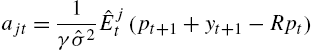
where γ is the coefficient of absolute risk aversion and ˆσ2![]() is the (perceived) conditional variance of excess returns. The risk parameter ˆσ
is the (perceived) conditional variance of excess returns. The risk parameter ˆσ![]() is pinned down as an equilibrium object of the model. As in the previous section, assume that there are two-types of agents who differ based on whether they forecast with a dividends-based or share supply-based model. Then market equilibrium requires that
is pinned down as an equilibrium object of the model. As in the previous section, assume that there are two-types of agents who differ based on whether they forecast with a dividends-based or share supply-based model. Then market equilibrium requires that
na1t+(1−n)a2t=At
where, again, At![]() represents asset share supply (or, float). The equilibrium process for price is, then, given by
represents asset share supply (or, float). The equilibrium process for price is, then, given by
(19) pt=β[nˆE1tpt+1+(1−n)ˆE2tpt+1]+βρyt−βaˆσ2At
where β=1/R![]() . As before, assume that dividends and share supply are represented as stationary AR(1) processes, written in deviation-from-mean form:
. As before, assume that dividends and share supply are represented as stationary AR(1) processes, written in deviation-from-mean form:
yt=(1−ρ)y0+ρyt−1+εtAt=(1−ϕ)A0+ϕAt−1+νt
Traders are assumed to form their forecasts by selecting from one of the following misspecified models:
PLM1:pt=b10+b1yt+ηtPLM1:pt=b20+b2At+ηt
where ηt![]() is a perceived white noise error. As before, the distribution of agents, after selecting their predictor, is given by the MNL map:
is a perceived white noise error. As before, the distribution of agents, after selecting their predictor, is given by the MNL map:
Tω(n)=12{tanh[ω2F(n)]+1}
A Misspecification Equilibrium is a fixed point n⁎![]() to the T-map, i.e. n⁎=Tω(n⁎)
to the T-map, i.e. n⁎=Tω(n⁎)![]() .
.
Branch and Evans (2010) show theoretically that there can exist multiple misspecification equilibria. An example is given in Fig. 3, which is based on a calibrated version of the model with ω→∞![]() . Fig. 3 plots the T-map and F(n)
. Fig. 3 plots the T-map and F(n)![]() functions, where the T-map crosses the 45∘
functions, where the T-map crosses the 45∘![]() line is a Misspecification Equilibrium. In the calibrated version of the model, there are multiple misspecification equilibria. When all agents use forecast model 1, then it is a best-response for an agent to use forecast model 1 as it delivers a lower mean-square forecast error. Similarly, for model 2. Notice that there is also an interior equilibrium exhibiting Intrinsic Heterogeneity. The right hand panels compute the volatility of returns for a given n. These figures reveal that there exist multiple misspecification equilibria, that differ in mean returns and volatilities. In particular, there exists a low return-low volatility and a high return-high volatility equilibrium.
line is a Misspecification Equilibrium. In the calibrated version of the model, there are multiple misspecification equilibria. When all agents use forecast model 1, then it is a best-response for an agent to use forecast model 1 as it delivers a lower mean-square forecast error. Similarly, for model 2. Notice that there is also an interior equilibrium exhibiting Intrinsic Heterogeneity. The right hand panels compute the volatility of returns for a given n. These figures reveal that there exist multiple misspecification equilibria, that differ in mean returns and volatilities. In particular, there exists a low return-low volatility and a high return-high volatility equilibrium.

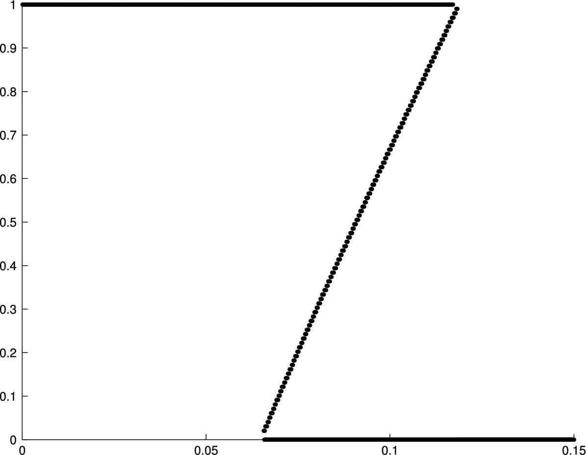
The set of Misspecification Equilibria depends on the structural parameters of the model. In particular, the degree of risk-aversion – analogously, in the search-based model, the preferences for the differentiated good – plays an important role in determining whether multiple equilibria and whether Intrinsic Heterogeneity can exist. In Fig. 4, Branch and Evans (2010) compute the misspecification equilibria treating the degree of risk-aversion, a, as a bifurcation parameter. For low and high risk aversion there exist unique equilibria with homogeneous expectations. For moderate, and empirically realistic, degrees of risk-aversion there are multiple equilibria, including ones with Intrinsic Heterogeneity.
Branch and Evans (2010) exploited the existence of multiple misspecification equilibria to generate regime-switching returns and volatilities that match those estimated in the data by Guidolin and Timmermann (2007). To generate plausible dynamics, the Misspecification Equilibrium values for the belief parameters bj![]() , and the mean-square errors, were replaced by real-time recursive econometric estimators. Branch and Evans also specified a recursive estimator for the conditional variance ˆσ2
, and the mean-square errors, were replaced by real-time recursive econometric estimators. Branch and Evans also specified a recursive estimator for the conditional variance ˆσ2![]() . The intensity of choice parameter was also calibrated to a finite value in order to match the Guidolin–Timmermann statistics. Fig. 5 illustrates a typical simulation that exhibits regime-switching returns and volatilities. As the distribution of heterogeneity n evolves in real-time, agents' beliefs fluctuate between neighborhoods of the low return/low volatility and high return/high volatility Misspecification Equilibria. Thus, misspecification and heterogeneity can lead to endogenous recurring regime switching asset returns.
. The intensity of choice parameter was also calibrated to a finite value in order to match the Guidolin–Timmermann statistics. Fig. 5 illustrates a typical simulation that exhibits regime-switching returns and volatilities. As the distribution of heterogeneity n evolves in real-time, agents' beliefs fluctuate between neighborhoods of the low return/low volatility and high return/high volatility Misspecification Equilibria. Thus, misspecification and heterogeneity can lead to endogenous recurring regime switching asset returns.
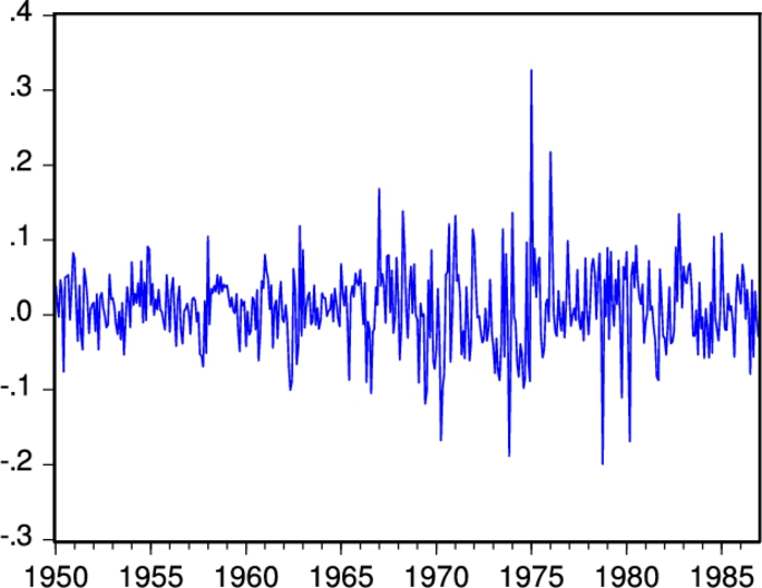
4.2 Bubbles with Rationally Heterogeneous Expectations
Beginning with Brock and Hommes (1998), a large literature has developed studying paths from rationally heterogeneous expectations to excess volatility, bubbles, and crashes in otherwise standard asset-pricing models. Much of this literature is surveyed in Hommes (2013), with special attention to identifying simple forecasting heuristics that are consistent with learning-to-forecast experiments in asset pricing and other experimental economies. To illustrate the main mechanics, we turn now to a version of the model (19), but where agents choose between rational and adaptive expectations.
Consider a non-stochastic version of (19):
pt=μ+β[nt−1ˆE1tpt+1+(1−nt−1)ˆE2tpt+1]
where μ=βˉy−aσ2ˉA![]() , and we assume the following expectations operators:
, and we assume the following expectations operators:
ˆE1tpt+1=pt+1ˆE2tpt=ˉp+θ(pt−1−ˉp)ˆE2tpt+1=ˉp+θ2(pt−1−ˉp)
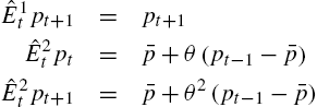
Predictor 1 is rational expectations (perfect foresight) and predictor 2 is an adaptive predictor that forecasts future prices as deviations from steady-state. Predictor 2 is an “anchor and adjustment” rule of the type that Hommes (2013) finds fits many experimental subjects' forecasts from the laboratory. In the example of this section, we assume that θ>1![]() , so that agents who use this predictor are strongly extrapolative. Notice also that we have explicitly assumed a time-varying weight on n while preserving the typical t−1
, so that agents who use this predictor are strongly extrapolative. Notice also that we have explicitly assumed a time-varying weight on n while preserving the typical t−1![]() -dating convention that forecasts made at time t are conditional on all information available through time t. This timing assumption breaks the simultaneity of expectations and equilibrium outcomes that are a defining feature of rational expectations equilibria but are not cognitively consistent in a model of bounded rationality. We also continue to assume that the distribution of predictor selection is given by the MNL map.
-dating convention that forecasts made at time t are conditional on all information available through time t. This timing assumption breaks the simultaneity of expectations and equilibrium outcomes that are a defining feature of rational expectations equilibria but are not cognitively consistent in a model of bounded rationality. We also continue to assume that the distribution of predictor selection is given by the MNL map.
Given these assumptions, the actual law of motion for this economy is given by the following pair of non-linear difference equations:
pt=ˆμ+(1βnt−1)pt−1−(1−nt−1nt−1)θ2pt−2nt=12{tanh[ω2(U1t−U2t)]+1}
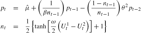
where ˆμ=−(βn)−1μ−(1−nt−1)(1−θ2)ˉp/nt−1![]() and U1t−U2t=(pt−ˆE2t−1pt)2−C
and U1t−U2t=(pt−ˆE2t−1pt)2−C![]() . For illustrative purposes, we measure predictor fitness as inversely related to the most recent squared forecast error net of the predictor cost, with the cost to using the adaptive predictor normalized to zero.
. For illustrative purposes, we measure predictor fitness as inversely related to the most recent squared forecast error net of the predictor cost, with the cost to using the adaptive predictor normalized to zero.
Fig. 6 plots a typical simulation that exhibits complex price dynamics. This figure was generating assuming θ=1.5,C=1,ω=2.6,β=0.95![]() , and μ=1
, and μ=1![]() . The first two panels plot the time paths for price and the fraction of rational agents along the stable attractor. The bottom panel plots the attractor in phase space. Price oscillates around the steady-state value with complex dynamics, featuring both excess volatility and bubbles/crashes. This simple example illustrates how rationally heterogeneous expectations can generate complex asset price dynamics. Other formulations of the predictors can lead to more realistic asset prices with larger bubbles and crashes, see, e.g. Hommes (2013) for examples.
. The first two panels plot the time paths for price and the fraction of rational agents along the stable attractor. The bottom panel plots the attractor in phase space. Price oscillates around the steady-state value with complex dynamics, featuring both excess volatility and bubbles/crashes. This simple example illustrates how rationally heterogeneous expectations can generate complex asset price dynamics. Other formulations of the predictors can lead to more realistic asset prices with larger bubbles and crashes, see, e.g. Hommes (2013) for examples.

The intuition for the complex dynamics arising from rationally heterogeneous expectations is based on attracting/repelling dynamics of predictor selection along with the stability reversal property discussed earlier. In this particular example, with forward- vs. backward-looking expectations, the steady-state is unstable when all agents adopt either rational or adaptive expectations. When the economy is close to steady-state the two predictors forecast equally well, so agents are unwilling to pay the cost for the rational predictor. This drives the economy away from the steady-state, i.e. the repelling dynamics. As price moves further from steady-state, the perfect foresight predictor's forecasting benefits begin to outweigh the cost, for some agents depending on their preference shocks, which balances the opposing repelling forces and tends to attract the system back towards the steady-state. These attracting/repelling forces combine to produce complex dynamics that can feature endogenous paths to bubbles and crashes.
4.3 Restricted Perceptions and Endogenous Fluctuations
A substantial body of research introduces volatility via fluctuations in expectations, for instance, through self-fulfilling sunspot shocks, news shocks, expectations shocks, sentiment shocks, forecasting add factors, exuberance shocks, etc. Broadly speaking, a drawback to these approaches to introducing expectations shocks, or animal spirits, is that it is difficult to construct instances where individuals and firms can coordinate their expectations. Branch and Zhu (2016), on the other hand, show how forecast model misspecification can expand the set of equilibria including restricted perceptions equilibria that depend on extrinsic noise. Interestingly, equilibria that depend on extrinsic noise do not necessarily exhibit more volatility than equilibria that only depend on fundamental economic variables. This is in contrast with much of the extant literature. Branch and Zhu (2016) show, however, that heterogeneity in forecast model misspecification can lead to more volatile equilibria that depend on extrinsic noise.
To illustrate the approach consider again the simplified asset-pricing model (19) with the share-supply shocks shut down:
pt=β[nˆE1tpt+1+(1−n)ˆE2tpt+1]+γyt
and yt=ρyt−1+εt,0<ρ<1![]() and ε is i.i.d. N(0,σ2ε)
and ε is i.i.d. N(0,σ2ε)![]() . Branch and Zhu (2016) follow the behavioral learning equilibria approach developed in Hommes and Zhu (2014), who assume that the exogenous shocks, yt
. Branch and Zhu (2016) follow the behavioral learning equilibria approach developed in Hommes and Zhu (2014), who assume that the exogenous shocks, yt![]() , are unobservable to all agents and so they instead fit autoregressive models to pt
, are unobservable to all agents and so they instead fit autoregressive models to pt![]() , with the coefficients picked to ensure that the first autocorrelation of the data generating process and the approximating models coincide. In Branch and Zhu (2016) agents differ in a subset of their regressors, where the models can be thought of as ARMAX, so that agents may include more or less autoregressive terms, the fundamental exogenous variable y, or even moving average terms. The novelty in Branch and Zhu (2016) is that they also potentially include non-fundamental exogenous variables – loosely speaking, expectations shocks – in their forecasting model. To illustrate, we consider the simplest case in Branch and Zhu (2016):
, with the coefficients picked to ensure that the first autocorrelation of the data generating process and the approximating models coincide. In Branch and Zhu (2016) agents differ in a subset of their regressors, where the models can be thought of as ARMAX, so that agents may include more or less autoregressive terms, the fundamental exogenous variable y, or even moving average terms. The novelty in Branch and Zhu (2016) is that they also potentially include non-fundamental exogenous variables – loosely speaking, expectations shocks – in their forecasting model. To illustrate, we consider the simplest case in Branch and Zhu (2016):
PLM1:pt=bpt−1+dηtPLM2:pt=cyt+fηt
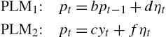
where ηt=ϕηt−1+νt![]() . The first predictor fits price to an AR(1) model plus a component common to the second predictor. The second predictor assumes these agents can observe the fundamental shocks, but also includes the common shock. The ηt
. The first predictor fits price to an AR(1) model plus a component common to the second predictor. The second predictor assumes these agents can observe the fundamental shocks, but also includes the common shock. The ηt![]() can be thought of as all other information, exogenous to the fundamentals of the asset-pricing economy, i.e. a statistical sunspot variable. Whether agents coordinate on the ηt
can be thought of as all other information, exogenous to the fundamentals of the asset-pricing economy, i.e. a statistical sunspot variable. Whether agents coordinate on the ηt![]() shock is determined as an equilibrium outcome. With these perceived laws of motion, the actual law of motion can be written as
shock is determined as an equilibrium outcome. With these perceived laws of motion, the actual law of motion can be written as
(20) pt=α1pt−1+α2yt+α3ηt
for appropriately defined αj![]() , j=1,2,3
, j=1,2,3![]() that depend on the structural model parameters and, importantly, the belief coefficients b,c,d,f
that depend on the structural model parameters and, importantly, the belief coefficients b,c,d,f![]() and the fraction of agents using model 1, n. Assume that n is an exogenous parameter in the model. Notice from (20) that the two predictors are misspecified: model 1 underparameterizes by excluding the fundamental shocks while model 2 omits lagged prices.
and the fraction of agents using model 1, n. Assume that n is an exogenous parameter in the model. Notice from (20) that the two predictors are misspecified: model 1 underparameterizes by excluding the fundamental shocks while model 2 omits lagged prices.
Because the two forecast models are misspecified, the appropriate equilibrium concept is Restricted Perceptions Equilibrium (RPE). Let X1t=(pt−1,ηt)′,X2t=(yt,ηt)′![]() . Then, in an RPE the beliefs satisfy the least-squares orthogonality conditions:
. Then, in an RPE the beliefs satisfy the least-squares orthogonality conditions:
EX1t[pt−(b,d)X1t]=0EX2t[pt−(c,f)X2t]=0

If n=1![]() and the RPE value d=0
and the RPE value d=0![]() then the equilibrium value of b coincides with the behavioral learning equilibrium in Hommes and Zhu (2014). If n=0
then the equilibrium value of b coincides with the behavioral learning equilibrium in Hommes and Zhu (2014). If n=0![]() then there is a unique RPE value f=0
then there is a unique RPE value f=0![]() and the value of c is the same as the rational expectations equilibrium coefficient. However, when n=1
and the value of c is the same as the rational expectations equilibrium coefficient. However, when n=1![]() Branch and Zhu (2016) show that there can also exist non-fundamental RPE with d≠0
Branch and Zhu (2016) show that there can also exist non-fundamental RPE with d≠0![]() . Thus, we focus on when 0<n⩽1
. Thus, we focus on when 0<n⩽1![]() .
.
Branch and Zhu (2016) show that there always exists fundamental RPE where d=0![]() and f=0
and f=0![]() . In this case, the associated mappings from perceived parameters (b,c)
. In this case, the associated mappings from perceived parameters (b,c)![]() to their least-squares projection values, computed using the implied actual law of motion, i.e. the “T-map” are
to their least-squares projection values, computed using the implied actual law of motion, i.e. the “T-map” are
b→b2nβ+ρ1+b2nβρc→1+c(1−n)βρ1−b2nβρ

The fundamental RPE reveals an important insight for the existence of the non-fundamental RPE. In this simple example, the second perceived law of motion is only misspecified because of n>0![]() , i.e. the presence of the agents who do not observe or forecast with the dividend shocks as a regressor. The existence of these agents, though, alters the serial correlation properties of asset prices, which because of the cross-equation restrictions associated to the RPE least-squares orthogonality condition, impacts the regression coefficient c of the type-2 agents. Thus, the misspecification alters the equilibrium weight on the exogenous shocks.
, i.e. the presence of the agents who do not observe or forecast with the dividend shocks as a regressor. The existence of these agents, though, alters the serial correlation properties of asset prices, which because of the cross-equation restrictions associated to the RPE least-squares orthogonality condition, impacts the regression coefficient c of the type-2 agents. Thus, the misspecification alters the equilibrium weight on the exogenous shocks.
Now consider the case where d,f≠0![]() . Such equilibria can arise when the feedback effects in the model are strong, i.e. when β is close to one, a condition that will be satisfied in most asset-pricing models. In particular, the T-map components for the coefficients b,c
. Such equilibria can arise when the feedback effects in the model are strong, i.e. when β is close to one, a condition that will be satisfied in most asset-pricing models. In particular, the T-map components for the coefficients b,c![]() now become
now become
b→1−βϕnβ(1−ϕ2)c→11−(1−n)βρ−b2nβρ
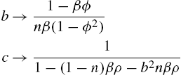
and d is pinned down by a complicated quadratic expression in the structural parameters n,β,ρ,ϕ![]() , and f→d/(1−βϕ)
, and f→d/(1−βϕ)![]() . The intuition for the existence of non-fundamental RPE is clear. The misspecification and heterogeneity introduce serial correlation in a temporary equilibrium sense. The agents optimally attribute some of that serial correlation to the endogenous variables – lagged prices for model 1 and serially correlated dividends for model 2 – and to the extrinsic variable ηt
. The intuition for the existence of non-fundamental RPE is clear. The misspecification and heterogeneity introduce serial correlation in a temporary equilibrium sense. The agents optimally attribute some of that serial correlation to the endogenous variables – lagged prices for model 1 and serially correlated dividends for model 2 – and to the extrinsic variable ηt![]() . The specific values of those regression coefficients depend on the distribution of agents across the two forecast models, as well as the stochastic properties of the shocks, i.e. ρ,ϕ
. The specific values of those regression coefficients depend on the distribution of agents across the two forecast models, as well as the stochastic properties of the shocks, i.e. ρ,ϕ![]() . Importantly, the non-fundamental RPE are self-fulfilling equilibria that only arise when expectations play an important role in the pricing equation. There are, therefore, three important ingredients for the existence of these non-fundamental equilibria: misspecification, heterogeneity, and strong expectational feedback.
. Importantly, the non-fundamental RPE are self-fulfilling equilibria that only arise when expectations play an important role in the pricing equation. There are, therefore, three important ingredients for the existence of these non-fundamental equilibria: misspecification, heterogeneity, and strong expectational feedback.
Fig. 7 illustrates the existence of the full set of RPE, including those depending on the statistical sunspots. This figure contains contour plots for the (b,c)![]() components of the T-map.9 The Td
components of the T-map.9 The Td![]() component consists of a horizontal line at d=0
component consists of a horizontal line at d=0![]() and another vertical line at the non-fundamental value for b. The Tb
and another vertical line at the non-fundamental value for b. The Tb![]() mapping is the parabolic lines in the figure. The figure illustrates the fixed points to the T-map for two different values of n. The n=1
mapping is the parabolic lines in the figure. The figure illustrates the fixed points to the T-map for two different values of n. The n=1![]() T-maps provide the existence of RPE without heterogeneity, while the n=0.9
T-maps provide the existence of RPE without heterogeneity, while the n=0.9![]() consists of some degree of heterogeneous expectations. Notice that a fundamental RPE exists in both cases and that the RPE value of b are very close to each other for both values of n. For both values of n, there exist two non-fundamental RPE, symmetric around the d=0
consists of some degree of heterogeneous expectations. Notice that a fundamental RPE exists in both cases and that the RPE value of b are very close to each other for both values of n. For both values of n, there exist two non-fundamental RPE, symmetric around the d=0![]() line. Increasing the degree of heterogeneity shifts the Td
line. Increasing the degree of heterogeneity shifts the Td![]() line to the right, implying higher degrees of perceived autocorrelation. Similarly, the Tb
line to the right, implying higher degrees of perceived autocorrelation. Similarly, the Tb![]() shifts away from the d=0
shifts away from the d=0![]() line, implying a relatively greater weight placed on the extrinsic noise d.
line, implying a relatively greater weight placed on the extrinsic noise d.
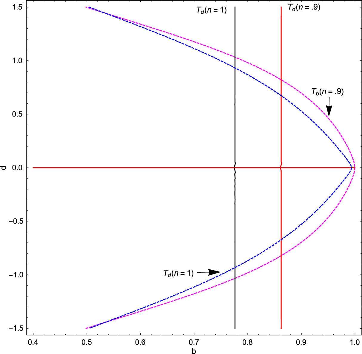
Branch and Zhu (2016) then ask the question of whether RPE that display dependence on extrinsic noise terms introduce more volatility into asset prices. It turns out that the effect is not obvious, as it depends on the equilibrium effect on all of the RPE belief coefficients. For example, bifurcating the equilibrium from a fundamental RPE to a non-fundamental RPE has a direct effect that increases asset-price volatility through the coordination of agents onto the extrinsic noise. However, there is a potentially competing effect on the equilibrium value for the AR(1) coefficient, b, in agents of type-one's forecasting model. These agents attribute, in part, some of the serial correlation in prices to the extrinsic term, lowering their estimated value of b, which will tend to push down asset-price volatility. Thus, the effect on volatility is a balancing of these two effects. See, for example, a particular numerical case in Branch and Zhu (2016) that is plotted in Fig. 8. This figure plots the ratio of RPE price volatility to the volatility in the rational expectations equilibrium as a function of the degree of heterogeneity, n, for both the fundamental RPE (solid) and non-fundamental RPE (dashed). This particular example is for a very strongly serially correlated process η. Depending on the degree of heterogeneity, the RPE can introduce excess volatility, but it is not necessarily the case. Moreover, for relatively high values of n, that are not too close to homogeneity, the excess volatility that arises from the non-fundamental RPE is greater than in the fundamental RPE. However, interestingly, when n=1![]() the excess volatility is greater in the fundamental RPE, which coincides with the equilibrium identified by Hommes and Zhu (2014). The intuition for these findings can be seen in Fig. 7. The equilibrium with heterogeneous expectations is more volatile than the n=1
the excess volatility is greater in the fundamental RPE, which coincides with the equilibrium identified by Hommes and Zhu (2014). The intuition for these findings can be seen in Fig. 7. The equilibrium with heterogeneous expectations is more volatile than the n=1![]() equilibrium because the autoregressive coefficient b and the weight placed on the sunspot d is relatively higher. Thus, to have statistical sunspots generate more volatility requires a self-reinforcing effect arising from heterogeneous expectations. However, if there is a sufficiently low n (n<0.85
equilibrium because the autoregressive coefficient b and the weight placed on the sunspot d is relatively higher. Thus, to have statistical sunspots generate more volatility requires a self-reinforcing effect arising from heterogeneous expectations. However, if there is a sufficiently low n (n<0.85![]() in the figure) then the non-fundamental RPE again produces less economic volatility. The reason is that as n decreases the Td
in the figure) then the non-fundamental RPE again produces less economic volatility. The reason is that as n decreases the Td![]() -map shifts to the right, and the forecasting models place less weight on both the sunspot (d,f)
-map shifts to the right, and the forecasting models place less weight on both the sunspot (d,f)![]() and the fundamental shock c.
and the fundamental shock c.

4.4 Related Literature
Much of the literature on asset-pricing in models with heterogeneous expectations was started by the seminal Brock and Hommes (1998), which applied the framework developed in Brock and Hommes (1997) to an asset pricing model where agents select between perfect foresight and a simple adaptive rule that nests extrapolative, contrarian, and trend-chasing expectations. These papers were inspired by LeBaron (1995) and other attempts at building artificial stock markets with heterogeneous, evolving technical trading strategies. Brock and Hommes (1998) demonstrated that rationally heterogeneous expectations could feature “a rational route to randomness” in asset prices for a wide specification of expectations-types. This launched an extensive literature with key contributions by Hommes and co-authors at the CENDEF at the University of Amsterdam. Important extensions include the “large-type limit” introduced by Brock et al. (2005), where agents select from a continuum of predictors, which has a natural Bayesian interpretation.
Importantly, this literature tackled the empirical foundations of heterogeneous expectations beyond their theoretical implications. A paper by Hommes et al. (2005) introduced “learning to forecast” experiments as a way to test for heterogeneous expectations in a simple laboratory environment. In this paper, a simple asset-pricing framework similar to Brock and Hommes (1998) was set in a laboratory where the only decision subjects were required to make was a forecast of the asset price in the next period, which automatically determines their portfolio allocation. Hommes et al. showed that the lab featured asset price dynamics that often converged to cycles around the fundamental price, i.e. bubbles and crashes. Moreover, they found that the best fit to the set of individual prediction strategies was a heterogeneous collection of simple autoregressive forecasting rules. Subsequent experiments across a range of model environments provide further evidence for heterogeneous beliefs and rationally evolving fractions of lab participants distributed across forecasting models. See, for instance, Hommes (2013) and Anufriev et al. (2015) for an extensive review.
There is also a literature that considers heterogeneity and adaptive learning. The seminal Marcet and Sargent (1989) featured a setting where agents had private information that creates for the other agents “hidden state variables,” but differed in which sets of variables were unobservable. They focused on convergence to a limited information rational expectations equilibrium. Subsequent papers, such as Marcet and Sargent (1995), examine where agents fit heterogeneous ARMA models, similar to the class of forecasting models in Branch and Zhu (2016). Guse (2005) studies an environment with agents who have heterogeneous expectations derived from forecasting rules that fit the full set of rational expectations equilibria, i.e. one rule is based on the minimal state variable solution while the other is for an ARMA with sunspot, and derives conditions under which the MSV equilibrium is stable under learning in a general environment. Similarly, Berardi (2007) extends that framework to forward-looking models with a lag that nests the asset-pricing model considered here.
Besides Branch and Evans (2010), there have been other heterogeneous expectations models of adaptive learning and asset-pricing. LeBaron (2012) constructs a model with constant gain learning where agents differ in their gain size, i.e. their robustness to structural change of an unknown form. Markiewicz (2012) considers a form of misspecification equilibrium, where the distribution across predictors is determined by running statistical specification tests based on the Kullback–Leibler information criterion, and applies it to explaining exchange rate puzzles. Nakov and Nuno (2015) apply the learning-from-experience model of Malmendier and Nagel (2016) to an asset-pricing model. Finally, Parke and Waters (2007) construct an evolutionary model of learning that endogenously generates ARCH effects in asset-prices. Elias (2016) includes expectations shocks into an asset-pricing model with heterogeneous learning.
5 Monetary Applications
There is an extensive literature in monetary theory that studies the role of money as a medium of exchange. The modern workhorse monetary model is the Lagos–Wright New Monetarist framework which is equivalent to the model of Section 2 when the asset is reinterpreted as fiat money, i.e. the asset has zero payoff flows and is intrinsically worthless. Fiat money has value in the New Monetarist framework because the agents in the economy coordinate on a rational expectations equilibrium where fiat money is valued as a medium of exchange precisely because they expect that it will have value in the future. However, there is also an autarky equilibrium. Baranowski (2015) shows that when agents are homogeneous and adaptively learn about the value of money, the monetary equilibrium is locally stable. Branch and McGough (2016) study the implications for monetary equilibria when agents have rationally heterogeneous expectations. They find that heterogeneous expectations have unique implications for trading efficiencies and the nature of trade in over-the-counter markets.
In particular, heterogeneous beliefs can account for some of the puzzling results in Duffy and Puzzello (2014), which are easily interpretable once the homogeneous expectations assumption is relaxed. From a theoretical perspective, this section shows how heterogeneous beliefs affect consumption and trade precisely because heterogeneity makes higher-order beliefs matter in a fundamental way, but only along dynamic paths. Therefore, the results surveyed here demonstrate that the type of dynamics highlighted in this survey can fundamentally alter economic mechanisms.
5.1 A Monetary Search Model with Heterogeneous Expectations
We begin by turning the preference shock, interpretable as a search friction, back on. With probability σ a buyer in the specialized good market will meet a seller. In this environment, the solution usually proceeds recursively, taking as given beliefs about the future. To set the stage, we turn to how a recursive solution can be found by starting with solving for equilibrium in the specialized goods sector. Following Branch and McGough (2016) we assume that the terms of trade are determined via take-it-or-leave-it offers made by buyers. If agents in this market are anonymous, buyers will be unable to commit to repaying any credit issued from sellers and all trade must be quid pro quo, i.e. the buyer must present a payment instrument, or equivalently, use an asset as collateral for a loan from the seller until the buyer receives proceeds from producing in the general goods market. We assume the existence of a single liquid asset, fiat money, which is a special case of the general framework where the asset has a zero payment flow, i.e. it is intrinsically worthless.
Buyers will decide on their asset holdings based on the discounted expected payoff of the asset, in terms of the general good, plus any expected liquidity services they provide. The literature has a number of ways of approaching how they decide on these asset holdings and consumption plans, depending on their beliefs about the future. To see this, denote by V(a)![]() the value function for a buyer at the beginning of the period before entering the specialized goods market. It is straightforward to see, using our earlier notation, that
the value function for a buyer at the beginning of the period before entering the specialized goods market. It is straightforward to see, using our earlier notation, that
Vt(at)=maxϕtqt⩽ptat/wtσ[u(qt)−ptqt]+ptatwt+Wt(0)
and, the Bellman equation for the agent is
W(at)=maxxt,ht,at+1v(xt)−ht+βˆEtVt+1(at+1)
subject to
xt+ptat+1=ptat+wtht
and qt=q(ptat)![]() . The next section determines q(⋅)
. The next section determines q(⋅)![]() through bilateral bargaining in the specialized goods market. Now let at=mt
through bilateral bargaining in the specialized goods market. Now let at=mt![]() denote holdings of real-money balances. Here we adopt the Bellman-equation learning approach, though with the quasi-linearity of the utility function, the asset-pricing equation is the same regardless of the assumed agent-level behavior. Because the value function is linear in wealth, the household chooses x so that v′(xt)=1/wt=1
denote holdings of real-money balances. Here we adopt the Bellman-equation learning approach, though with the quasi-linearity of the utility function, the asset-pricing equation is the same regardless of the assumed agent-level behavior. Because the value function is linear in wealth, the household chooses x so that v′(xt)=1/wt=1![]() . The next section describes the implications of heterogeneous beliefs for bargaining and trade, and then optimal asset holdings.
. The next section describes the implications of heterogeneous beliefs for bargaining and trade, and then optimal asset holdings.
5.2 Heterogeneous Beliefs and Bargaining
The departure point from Lagos and Wright (2005) in Branch and McGough (2016) is the common knowledge assumptions during trade between buyers and sellers. To illustrate the implications of heterogeneous beliefs for trading inefficiencies, we make two small changes to the benchmark model of Section 2: first, we assume the asset is fiat money, i.e. yt=0![]() ; second, we assume, like Lagos and Wright, that the differentiated good is traded in a decentralized market with search frictions. That is, we assume that in each decentralized market a buyer and seller are matched with probability σ. Trades in these markets are still subject to the limited commitment friction that precludes the use of unsecured credit. Once buyers and sellers are matched they bargain over the terms of trade, i.e. how much fiat money a buyer gives to a seller in exchange for a quantity of the specialized good. Branch and McGough (2016) focus on the set-up where buyers make take-it-or-leave-it offers as a natural way to relax common knowledge assumptions.
; second, we assume, like Lagos and Wright, that the differentiated good is traded in a decentralized market with search frictions. That is, we assume that in each decentralized market a buyer and seller are matched with probability σ. Trades in these markets are still subject to the limited commitment friction that precludes the use of unsecured credit. Once buyers and sellers are matched they bargain over the terms of trade, i.e. how much fiat money a buyer gives to a seller in exchange for a quantity of the specialized good. Branch and McGough (2016) focus on the set-up where buyers make take-it-or-leave-it offers as a natural way to relax common knowledge assumptions.
Assume as in Section 4.2 that buyers have rationally heterogeneous expectations: at the end of each period, after all markets clear, buyers choose their predictor for the following period. Then, in the subsequent period, given those beliefs, buyers and sellers are matched and buyers make a take-it-or-leave-it offer. Without loss of generality, Branch and McGough assume that sellers have perfect foresight. Thus, when a buyer is deciding on their money holdings they must forecast the value of money in the next period and the probability of actually trading in the decentralized market. The probability of trading depends on sellers' beliefs, which are assumed to not be common knowledge within a match. Thus, each buyer's predictor is assumed to have two components: point forecasts pet+1(j)![]() and a bargaining uncertainty measure Fjt+1(⋅,Σ),j=1,2
and a bargaining uncertainty measure Fjt+1(⋅,Σ),j=1,2![]() . A buyer of type-j believes with certainty that the value of money will be pet+1(j)
. A buyer of type-j believes with certainty that the value of money will be pet+1(j)![]() , in the following CM, in order to make an offer to the seller they must hold beliefs about sellers' beliefs. This is where bargaining uncertainty is important.
, in the following CM, in order to make an offer to the seller they must hold beliefs about sellers' beliefs. This is where bargaining uncertainty is important.
With take-it-or-leave it offers there is not an extended period of bargaining, the buyer simply makes an offer and the seller chooses to accept or reject. Without an extended interaction, buyers will not learn any useful information from sellers. Thus, it is natural to assume that buyers and sellers' beliefs are not common knowledge within a match. Instead, we assume that buyers use their own forecasts as proxies for the seller's beliefs. However, buyers behave like a good Bayesian who acknowledges his uncertainty and places a prior on the seller's forecasts via the distribution function Fjt(⋅,Σ)![]() , where the mean of the distribution is the buyer's own forecast pe(j)
, where the mean of the distribution is the buyer's own forecast pe(j)![]() and the variance, or uncertainty, is parameterized by Σ. Branch and McGough (2016) consider cases where Σ is taken to be a parameter, and where it is endogenous. As the buyers learn over time they update their prior distribution.
and the variance, or uncertainty, is parameterized by Σ. Branch and McGough (2016) consider cases where Σ is taken to be a parameter, and where it is endogenous. As the buyers learn over time they update their prior distribution.
A Bayesian offer balances the buyer maximizing his surplus against the subjective probability that the offer will be accepted. In particular, Branch and McGough (2016) show that Bayesian offers solve the following problem:
maxq,d⩽m(u(q)−pe(j)d)(1−FΣ(c(q)d))
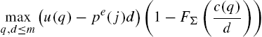
A buyer makes an offer of d units of money in exchange for q units of the specialized good in order to maximize the expected surplus given that the offer cannot exceed their holdings of money m, and the expectation is taken with respect to their subjective prior over the seller's acceptance rule. The first term in the objective is the buyer's surplus, and the second term is the subjective probability that the offer will be accepted. The seller accepts an offer in time t if and only if
ptd⩾c(q)
Branch and McGough (2016) show that Bayesian offers introduce caution into bargaining. Buyers, by acknowledging their uncertainty over the sellers' acceptance rule, demand fewer goods in exchange for their fiat money. While such offers sacrifice some surplus on the intensive margin, it raises the likelihood of trade on the extensive margin. Nevertheless, if buyers' beliefs are sufficiently different from sellers, the sellers may still reject the offer and heterogeneous beliefs can imply an extensive margin of trade that would not exist otherwise. Moreover, Branch and McGough derive the money-demand function for buyers and find that it depends on both the current price of money, expectations about future prices, and the uncertainty measure in their prior distribution. Thus, heterogeneity and uncertainty have important implications for the nature of trade, inflation and welfare.
5.3 Equilibrium with Heterogeneous Beliefs
Given the solution to the bargaining problem, and the definitions of the value functions, it follows that the optimal holdings of real-money balances solves:
maxmt+1{−(pt−βpet+1(τt))mt+1+βσ(1−FτtΣ(c(q(mt+1,pet+1(τt))d(mt+1,pet+1(τt))))×(u(q(mt+1,pet+1(τt)))−pet+1d(mt+1,pet+1(τt)))}
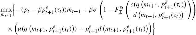
The money-demand function depends on whether the buyers' Bayesian offer liquidity constraint d⩽m![]() binds. If the constraint binds, so that pet+1(τt)<β−1pt
binds. If the constraint binds, so that pet+1(τt)<β−1pt![]() , then d=mt+1
, then d=mt+1![]() and mt+1
and mt+1![]() solves the interior F.O.C.
solves the interior F.O.C.
(21) 0=−pt+βpet+1(τt)+βσ(1−FτtΣ(c(q(mt+1,pet+1(τt)))mt+1))×(u′(q(mt+1,pet+1(τt)))×∂∂mt+1(q(mt+1,pet+1(τt)))−pet+1(τt))−βσdFτtΣ(c(q(mt+1,pet+1(τt)))mt+1)×∂∂mt+1(c(q(mt+1,pet+1(τt)))mt+1)
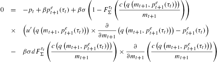
This implies a money-demand function of the form m(pt,pet+1(τ))![]() . Then an equilibrium price path is a sequence of prices pt
. Then an equilibrium price path is a sequence of prices pt![]() satisfying market clearing:
satisfying market clearing:
(22) N∑τ=1nt(τ,pt−1,{pet−1(ω)}Nω=1)m(pt,pet+1(τ))=M

5.4 Uncertainty and Welfare
Branch and McGough (2016) assume a form of rationally heterogeneous expectations that is the same as in Section 4.2, where agents select between a costly rational expectations predictor and an adaptive learning rule. Both predictors nest the steady-state, so the effects of heterogeneity and uncertainty only matter for out-of-steady-state dynamics. Branch and McGough (2016) show that the non-linear attracting/repelling dynamics that led to bubbles and crashes in Section 4.2 are at work in the monetary economy as well. For sufficient curvature in the utility function for specialized goods, i.e. a sufficiently large liquidity premium for money, there are periodic and aperiodic attractors that remain bounded around the monetary steady-state.
The extent to which buyers are cautious in their offers to sellers has important implications for welfare and economic dynamics. To illustrate this, we report on the experiments in Branch and McGough (2016). In that paper, they treat the uncertainty measure Σ as a bifurcation parameter and calculate welfare, offers, and acceptance rates along a stable attractor. Figs. 9 and 10 plot the results of a particular numerical example.
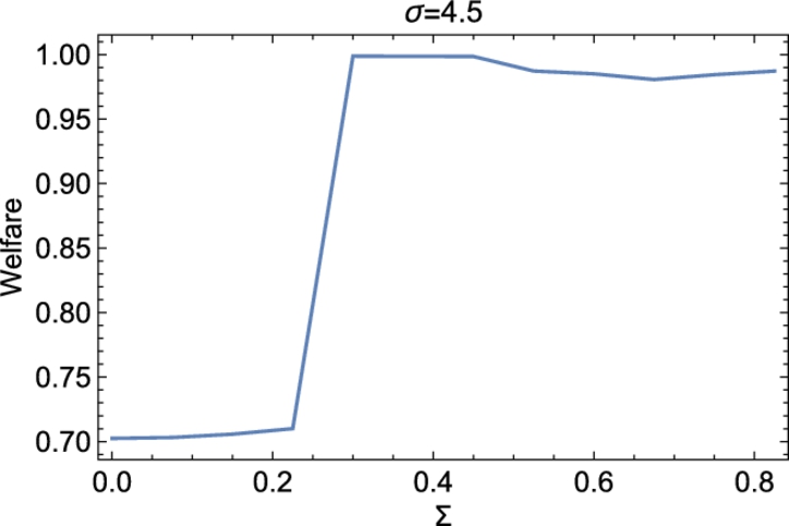
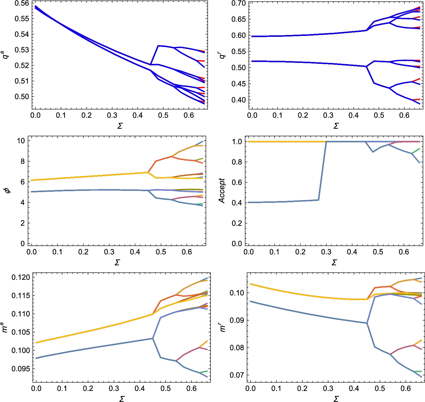
In Fig. 9 average welfare, relative to the rational expectations equilibrium, is calculated along a stable attractor, with the values of the specific variables plotted as a series of bifurcation plots in Fig. 10. In the center-left panel of Fig. 10 it is evident that for low values of Σ price is following a 2-cycle. As price fluctuates, the expectations of buyers with adaptive beliefs fluctuates as well, and they, in alternating periods, under-estimate the seller's willingness to accept the terms of their offer implying that the acceptance rate follows a 2-cycle (center-right). However, buyers introduce more caution into their offers as Σ increases (top-left) and so the average acceptance rate increases along the two-cycle. In Fig. 9 this shows up as an increase in welfare, though welfare is always below what would arise under homogeneous beliefs. At Σ≈0.30![]() , a threshold is crossed where offers are sufficiently cautious that the acceptance rate becomes one. In Fig. 9 this appears as a large increase in welfare accompanying the increase in the extensive margin of trade between heterogeneous agents. Then, conditional on the two-cycle, further increases in the uncertainty parameter only have a negative effect on the intensive margin and so welfare increases. Eventually, there is another bifurcation, with a 4-cycle appearing, an average acceptance rate below one, and a decrease in welfare.
, a threshold is crossed where offers are sufficiently cautious that the acceptance rate becomes one. In Fig. 9 this appears as a large increase in welfare accompanying the increase in the extensive margin of trade between heterogeneous agents. Then, conditional on the two-cycle, further increases in the uncertainty parameter only have a negative effect on the intensive margin and so welfare increases. Eventually, there is another bifurcation, with a 4-cycle appearing, an average acceptance rate below one, and a decrease in welfare.
These results illustrate how heterogeneous beliefs can lead to new dynamic phenomena. In many settings, differences in information can lead to more trading opportunities. In this setting, heterogeneous beliefs and uncertainty play subtle roles in determining trading inefficiencies and welfare. More uncertainty leads to more cautious offers, lowering welfare through the intensive margin, while increase the likelihood of trade and welfare. Branch and McGough (2016), though, show the importance that common knowledge assumptions play in trade between agents with heterogeneous expectations.
Branch and McGough also applied their model to help explain key puzzles in the experimental findings of Duffy and Puzzello (2014), who find laboratory support for the Lagos–Wright monetary theory. They also find, however, that
- 1. a large fraction of offers made by buyers are not accepted by sellers;
- 2. the accepted offers are different from the theoretical stationary equilibrium price and quantity;
- 3. there is a non-degenerate distribution of money holdings despite evidence of portfolio rebalancing in the centralized market;
- 4. higher-quantity (buyer) offers are more likely to be rejected.
These experimental results are consistent with the theoretical predictions of the monetary search model with heterogeneous expectations that is surveyed here. Furthermore, the model presented in this paper makes sharp predictions regarding the relationship between prices and the acceptance rate, as well as between prices and sellers' realized surpluses, which should be invariant to the price of money under rational expectations. These findings all present further empirical support for the role of heterogeneous expectations in macroeconomic models.
5.5 Related Literature
While there is an active literature incorporating heterogeneous private information into monetary search environments, see Rocheteau and Nosal (2017), there have been few studies incorporating bounded rationality into the search environments. Baranowski (2015) was the first to introduce adaptive learning and showed how stability of a monetary equilibrium can arise when agents have homogeneous adaptive learning rules. Branch (2016) studied the asset-pricing implications of a form of extrinsic heterogeneity, where asset-holders form expectations about future asset prices with a real-time adaptive learning rule and firms have perfect foresight. Similarly, Branch et al. (2016) also features extrinsic heterogeneity in a two-sector model with labor and goods market search frictions, with workers and firms in different sectors having heterogeneous learning rules.
6 DSGE Applications
A burgeoning literature, beginning with Branch and McGough (2009) and Branch and McGough (2010), examines the implications of heterogeneous expectations in New Keynesian and Real Business Cycle models. A takeaway from this literature is that heterogeneous expectations alters the propagation mechanism of exogenous shocks and the transmission of monetary policy. This section provides an overview by focusing on the implications for the design of monetary policy rules.
6.1 Rationally Heterogeneous Expectations and Monetary Policy Rules
The companion papers, Branch and McGough (2009) and Branch and McGough (2010), develop a theory of heterogeneous expectations in a New Keynesian model. In Branch and McGough (2009) conditions on the set of admissible heterogeneous expectations operators are derived that facilitates aggregation of heterogeneous individual agent behavior that leads to equilibrium conditions that have the same form as the familiar IS and AS relations in New Keynesian models. That paper shows that once the benchmark model is extended to include heterogeneity, the usual ‘Taylor Principle’ is not necessary or sufficient for monetary policy to guarantee determinacy of equilibrium. Branch and McGough (2010) extend the analysis to where there are rationally heterogeneous expectations and shows that even for monetary policy rules satisfying the Taylor principle it is possible for there to be inefficiently volatile periodic and complex dynamics.
Branch and McGough (2009) derive the following pair of equilibrium equations governing the evolution of the economy:
(23) yt=ˆEtyt+1−υ−1(it−ˆEtπt+1)πt=βˆEtπt+1+λyt

where yt![]() is the output gap, πt
is the output gap, πt![]() is the inflation rate, it
is the inflation rate, it![]() is the nominal interest rate on one-period bonds and is the policy rate. All variables are in log-deviation from steady-state. The expectations operator ˆE
is the nominal interest rate on one-period bonds and is the policy rate. All variables are in log-deviation from steady-state. The expectations operator ˆE![]() is a linear combination of the individual heterogeneous expectations operators. The parameters υ>0
is a linear combination of the individual heterogeneous expectations operators. The parameters υ>0![]() is the intertemporal elasticity of substitution, 0<β<1
is the intertemporal elasticity of substitution, 0<β<1![]() is the discount rate, and λ is an expression of other structural parameters including the degree of price rigidity. The first line in (23) is the so-called IS equation, which relates aggregate demand in the current period to expected future demand and the ex-ante real interest rate. The second line in (23) is the New Keynesian Phillips curve which describes inflation as a function of discounted expected future inflation and the current output gap. Branch and McGough (2009) provide an axiomatic foundation to the expressions in (23). In addition, Branch and McGough also invoke two further axioms:
is the discount rate, and λ is an expression of other structural parameters including the degree of price rigidity. The first line in (23) is the so-called IS equation, which relates aggregate demand in the current period to expected future demand and the ex-ante real interest rate. The second line in (23) is the New Keynesian Phillips curve which describes inflation as a function of discounted expected future inflation and the current output gap. Branch and McGough (2009) provide an axiomatic foundation to the expressions in (23). In addition, Branch and McGough also invoke two further axioms:
- A6. If x is a variable forecasted by agents at time t and time t+k then EτtEτ′t+k(xt+k)=Eτtxt+k
 , τ′≠τ
 .
. - A7. All agents have common expectations on expected differences in limiting wealth.
These additional restrictions on expectations are the law of iterated expectations at an individual and aggregate level (A6) and vanishing heterogeneity in the long-run (A7). Finally, Branch and McGough consider a set of Taylor-type policy rules with an expectations-based rule as the benchmark:
(24) it=χπEtπt+1+χyEtyt+1
where here expectations are taken to be rational.
To illustrate the main results, we continue to maintain that expectations are the ones considered in Section 4.2, so that aggregate expectations are
ˆEtyt+1=nEtyt+1+(1−n)θ2yt−1ˆEtπt+1=nEtπt+1+(1−n)θ2πt−1
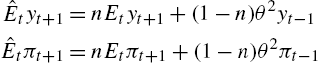
Notice that the steady-state values for y,π![]() are zero, and here we do impose type-1 expectations are rational but not necessarily perfect foresight.10 While previous sections focused on adaptive expectations, i.e. 0<θ⩽1
are zero, and here we do impose type-1 expectations are rational but not necessarily perfect foresight.10 While previous sections focused on adaptive expectations, i.e. 0<θ⩽1![]() , Branch and McGough (2009) develop results also considering the case where θ>1
, Branch and McGough (2009) develop results also considering the case where θ>1![]() , which is a case of extrapolative or trend-chasing expectations.
, which is a case of extrapolative or trend-chasing expectations.
Assuming, for the moment, that n is exogenously given, plugging in expectations and the policy rule into (23) leads to the reduced-form dynamical system
FXt=BEtXt+1+CXt−1
where X′=(y,π)![]() , and for appropriately conformable matrices F,B,C
, and for appropriately conformable matrices F,B,C![]() . This casts the heterogeneous expectations model into an associated rational expectations model. Since the associated rational model has the same form as a rational expectations model we can study the set of heterogeneous expectations equilibria by examining the determinacy properties of the associated model. In particular, the determinacy properties can be determined from the eigenvalues of the matrix
. This casts the heterogeneous expectations model into an associated rational expectations model. Since the associated rational model has the same form as a rational expectations model we can study the set of heterogeneous expectations equilibria by examining the determinacy properties of the associated model. In particular, the determinacy properties can be determined from the eigenvalues of the matrix
M=(B−1F−B−1CI20)

There are two pre-determined variables in the system and so the heterogeneous expectations model is determinate provided that there are two eigenvalues of M outside the unit circle. When there are fewer eigenvalues outside the unit circle then the model is indeterminate and can feature dependence on extrinsic noise or “sunspots.” If there are three eigenvalues inside the unit circle then the model has order-1 indeterminacy and the equilibrium depends on a single sunspot variable. If all eigenvalues are inside the unit circle then the model has order-2 indeterminacy and there is dependence on two sunspot variables.
The main insight in Branch and McGough (2009) is that heterogeneous expectations can alter the determinacy properties of a model with homogeneous expectations. In particular,
Result 4
- 1. If θ⩽1
 then policy rules that correspond to indeterminacy when n=1 may yield determinacy when there is even a small proportion of adaptive agents in the economy. In this sense, heterogeneous expectations may be stabilizing.
 - 2. If θ>1
 then policy rules that correspond to determinacy when n=1 may yield indeterminacy when there is even a small proportion of adaptive agents in the economy. In this case, heterogeneous expectations may be destabilizing.
That the optimal design of monetary policy rules hinges on the nature of heterogeneity and the details of how precisely households and firms form expectations is an important takeaway. Policy rules that are thought to stabilize the economy may actually destabilize, and vice versa, depending on the nature of how agents form expectations. Importantly, these findings arise for even small fractions of adaptive agents with most other people holding rational expectations.
An example of how heterogeneity affects the number and nature of equilibria is presented in Fig. 11, from Branch and McGough (2009). This figure plots the determinacy properties in the policy-rule space (χy,χπ)![]() . Each panel corresponds to a different proportion of rational agents n. The north-west plot is the determinacy properties under rational expectations which clearly demonstrates the Taylor principle: policy rules that are sufficiently active, i.e. χπ>1
. Each panel corresponds to a different proportion of rational agents n. The north-west plot is the determinacy properties under rational expectations which clearly demonstrates the Taylor principle: policy rules that are sufficiently active, i.e. χπ>1![]() and χy
and χy![]() not too large, lead to determinacy. However, as the degree of heterogeneity increases the diagonal line that determines the boundary between the determinate and indeterminate policy space, rotates clockwise. Policy rules that yield determinacy under rational expectations can lead to indeterminacy under heterogeneous expectations. Thus, the Taylor principle is not a necessary and sufficient condition for stability.
not too large, lead to determinacy. However, as the degree of heterogeneity increases the diagonal line that determines the boundary between the determinate and indeterminate policy space, rotates clockwise. Policy rules that yield determinacy under rational expectations can lead to indeterminacy under heterogeneous expectations. Thus, the Taylor principle is not a necessary and sufficient condition for stability.
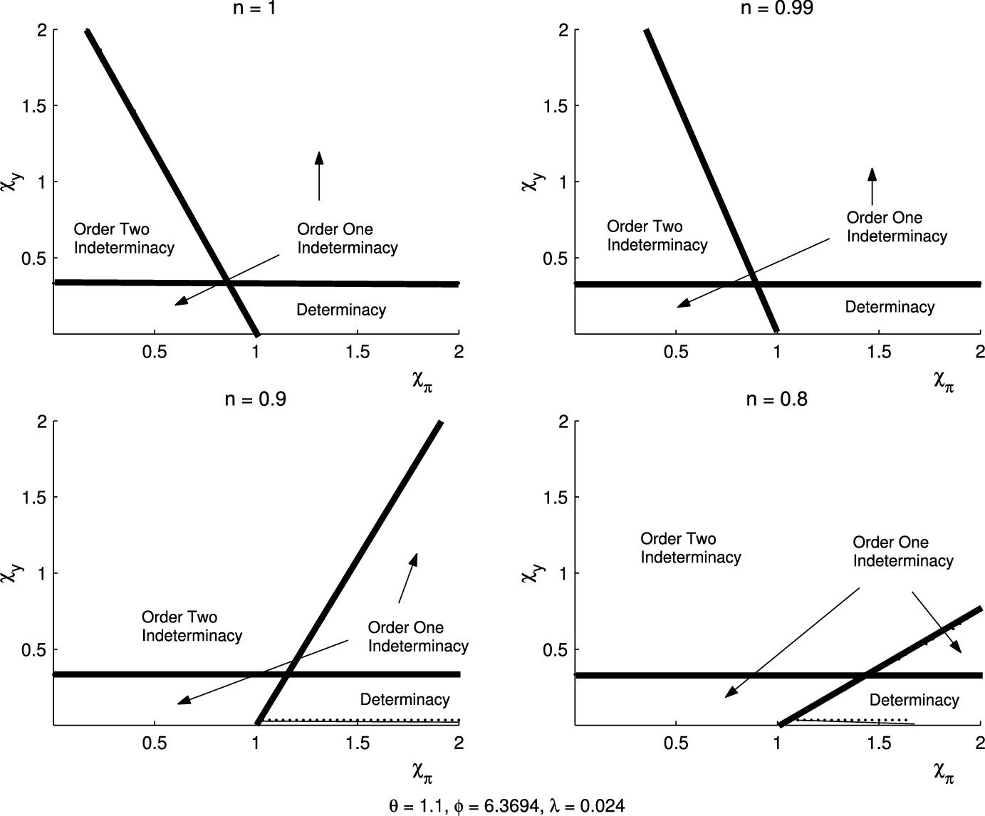
Fig. 11 also has important insights for the dynamics under rationally heterogeneous expectations, as shown in Branch and McGough (2010). The insight comes, again, from the stability reversal principle. Order-2 indeterminacy is equivalent to saying that the steady-state with rationally heterogeneous expectations, i.e. with the MNL map determining nt![]() in real-time, is locally stable. Order-1 indeterminacy, determinacy, and explosiveness when there are fewer contracting eigenvalues. Fig. 11 shows that as there are more adaptive agents in steady-state (for example by increasing the cost to using rational expectations C) that the steady-state can become stable. Branch and McGough (2010) show that if n becomes sufficiently small then the steady-state can become unstable with all eigenvalues outside the unit circle – this is the stability reversal property. Thus, as n fluctuates above and below the steady-state there can be the kind of attracting/repelling dynamics that lead to periodic and complicated dynamics. For example, suppose that the cost is sufficiently high so that there is a high proportion of adaptive agents and the steady-state is unstable. Then the dynamics will repel the system away from the steady-state. As the system moves away from the steady-state, the forecast errors for adopting rational expectations will be sufficiently lower than for the adaptive predictor that more and more agents will adopt the rational predictor. This moves the system into the “stable”, or indeterminacy type-2, region and attracts the dynamics back toward the steady-state. Near the steady-state, though, adaptive and rational expectations return very similar forecasts, the fraction of adaptive agents begins to increase, and the economy switches back into the unstable region. These attracting/repelling dynamics, depending on the steady-state value of adaptive agents, can lead to complex dynamics. For example, Fig. 12 plots a typical bifurcation diagram, where the cost of using rational expectations C is the bifurcation parameter.
in real-time, is locally stable. Order-1 indeterminacy, determinacy, and explosiveness when there are fewer contracting eigenvalues. Fig. 11 shows that as there are more adaptive agents in steady-state (for example by increasing the cost to using rational expectations C) that the steady-state can become stable. Branch and McGough (2010) show that if n becomes sufficiently small then the steady-state can become unstable with all eigenvalues outside the unit circle – this is the stability reversal property. Thus, as n fluctuates above and below the steady-state there can be the kind of attracting/repelling dynamics that lead to periodic and complicated dynamics. For example, suppose that the cost is sufficiently high so that there is a high proportion of adaptive agents and the steady-state is unstable. Then the dynamics will repel the system away from the steady-state. As the system moves away from the steady-state, the forecast errors for adopting rational expectations will be sufficiently lower than for the adaptive predictor that more and more agents will adopt the rational predictor. This moves the system into the “stable”, or indeterminacy type-2, region and attracts the dynamics back toward the steady-state. Near the steady-state, though, adaptive and rational expectations return very similar forecasts, the fraction of adaptive agents begins to increase, and the economy switches back into the unstable region. These attracting/repelling dynamics, depending on the steady-state value of adaptive agents, can lead to complex dynamics. For example, Fig. 12 plots a typical bifurcation diagram, where the cost of using rational expectations C is the bifurcation parameter.

6.2 Intrinsic Heterogeneity and Monetary Policy Rules
Monetary policy rules can also affect the number and nature of equilibria that agents coordinate on in stochastic environments. Branch and Evans (2011) embed the Misspecification Equilibrium framework in a New Keynesian model to see whether Intrinsic Heterogeneity and/or multiple misspecification equilibria can arise depending on the central bank's policy rule.
Branch and Evans (2011) consider a stochastic version of the New Keynesian model with heterogeneous expectations derived by Branch and McGough (2009):
(25) yt=ˆEtyt+1−σ−1(it−ˆEtπt+1)+gtπt=βˆEtπt+1+λyt+ut
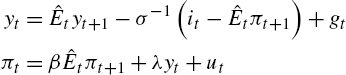
where gt=ρgt−1+εt![]() is a stationary stochastic process for “aggregate demand” shocks and ut=ϕut−1+νt
is a stationary stochastic process for “aggregate demand” shocks and ut=ϕut−1+νt![]() are “aggregate supply” shocks. The shocks g and u are (potentially) correlated, and ˆE
are “aggregate supply” shocks. The shocks g and u are (potentially) correlated, and ˆE![]() is an aggregate expectations operator to be specified below. Branch and Evans consider a variety of rules. Here we consider a rule that depends on contemporaneous private-sector expectations:
is an aggregate expectations operator to be specified below. Branch and Evans consider a variety of rules. Here we consider a rule that depends on contemporaneous private-sector expectations:
it=χπˆEtπt+χyˆEtyt
This rule is often advocated for as being close to the Taylor rule but depending on observable variables, in this case private-sector expectations. Branch and Evans show that the main qualitative results do not depend on the form of the policy rule.
As in Section 3.3, agents are assumed to underparameterize their forecasting models. In a determinate model, the rational expectations equilibrium depends linearly on the two shocks, g and u. The misspecification equilibrium approach assumes that agents prefer parsimony and instead select only the best-performing models from the set of underparameterized statistical models. Since there are only two stochastic driving variables, agents select from the following set of predictors, for variable x,
E1txt=b1gt,E1txt+1=b1ρgtE2txt=b2ut,E2txt+1=b2ϕut
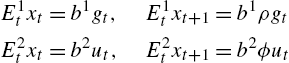
As usual, letting n denote the fraction that use forecast model 1, ˆEx=nE1x+(1−n)E2x![]() .
.
Plugging in expectations leads to a reduced-form actual law of motion
xt=ξ1(n)gt+ξ2(n)ut
The reduced-form expressions ξj![]() , j=1,2
, j=1,2![]() depend on the direct effect that gt,ut
depend on the direct effect that gt,ut![]() have on the economy, as well as the indirect effect that arises from the self-referential nature of the New Keynesian model. Thus, the distribution of agents across the two forecasting models depends on a balancing of the direct and indirect effects of the shocks. In a restricted perceptions equilibrium, the belief parameters bj
have on the economy, as well as the indirect effect that arises from the self-referential nature of the New Keynesian model. Thus, the distribution of agents across the two forecasting models depends on a balancing of the direct and indirect effects of the shocks. In a restricted perceptions equilibrium, the belief parameters bj![]() are pinned down to satisfy the least-squares orthogonality conditions
are pinned down to satisfy the least-squares orthogonality conditions
Egt(ξ1(n)gt+ξ2(n)ut−b1gt)=0Eut(ξ1(n)gt+ξ2(n)ut−b2ut)=0
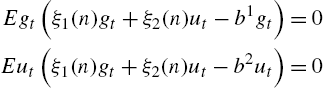
While the value of n is pinned down by the MNL map:
n=12{tanh[ωF(n)]+1}≡Tω(n)
where F(n)=EU1−EU2![]() and
and
EUj=−E(xt+k−Ejtxt+k)′W(xt+k−Ejtxt+k)
where W is a weighting matrix, set to the identity matrix without loss of generality. A Misspecification Equilibrium is a fixed point of the T-map: n⁎=Tω(n⁎)![]() . As before, the number and nature of equilibria depend on the function F(n)
. As before, the number and nature of equilibria depend on the function F(n)![]() .
.
Branch and Evans (2011) prove the following result, which makes use of the notation for the correlation coefficients r=Egtut/Eg2t,˜r=Egtut/Eu2t![]() .
.
Proposition 5
Let r,˜r![]() be sufficiently small and assume that the intensity of choice ω is large.
be sufficiently small and assume that the intensity of choice ω is large.
- 1. For ξπ
 , and/or ξy
 , sufficiently large, depending on σ2εσ2ν
 , there either exists a Misspecification Equilibrium with Intrinsic Heterogeneity, or there exists a Misspecification Equilibrium with n⁎=0
 .
. - 2. For σ2εσ2ν large, there exists a Misspecification Equilibrium with n⁎=0.
- 3. For σ2εσ2ν small, there exists a Misspecification Equilibrium with n⁎=1
 .
. - 4. For intermediate values, there exists multiple Misspecification Equilibria.
The restriction on the correlation coefficients ensures the existence of a unique RPE, given n. Then, the type of equilibria observed depends on the feedback of expectations through the policy rule, parameterized by the coefficients ξπ,ξy![]() . Similarly, the direct effect of the shocks, given by the ratio of the variances of their white noise shocks, affects whether there is an equilibrium with homogeneous expectations at either n⁎=0
. Similarly, the direct effect of the shocks, given by the ratio of the variances of their white noise shocks, affects whether there is an equilibrium with homogeneous expectations at either n⁎=0![]() or n⁎=1
or n⁎=1![]() , or multiple equilibria.
, or multiple equilibria.
Fig. 13 illustrates the possibilities in one particular numerical example from Branch and Evans (2011). The figure plots the bifurcation diagram where the central bank's reaction coefficient to inflation, χπ![]() is the bifurcating parameter. The figure considers values for χπ
is the bifurcating parameter. The figure considers values for χπ![]() that both satisfy and violate the Taylor principle. For weak central bank responses to inflation, there can exist multiple misspecification equilibria. Then for values just above the Taylor principle, there exists a unique misspecification equilibrium at n=1
that both satisfy and violate the Taylor principle. For weak central bank responses to inflation, there can exist multiple misspecification equilibria. Then for values just above the Taylor principle, there exists a unique misspecification equilibrium at n=1![]() , thus in accordance with case 3 in Proposition 5. Then as ξπ
, thus in accordance with case 3 in Proposition 5. Then as ξπ![]() becomes sufficiently large, as predicted by case 1 in Proposition 5, there exists a unique equilibrium exhibiting Intrinsic Heterogeneity. Thus, empirically realistic policy rule parameters can provide an explanation for heterogeneous expectations observed in survey data. The intuition is that they alter the feedback properties of the model so that a non-degenerate distribution of expectations-types will arise in equilibrium. For even larger values of χπ
becomes sufficiently large, as predicted by case 1 in Proposition 5, there exists a unique equilibrium exhibiting Intrinsic Heterogeneity. Thus, empirically realistic policy rule parameters can provide an explanation for heterogeneous expectations observed in survey data. The intuition is that they alter the feedback properties of the model so that a non-degenerate distribution of expectations-types will arise in equilibrium. For even larger values of χπ![]() multiple equilibria with Intrinsic Heterogeneity arises, and then eventually there is a unique equilibrium where all agents forecast with the supply shocks.
multiple equilibria with Intrinsic Heterogeneity arises, and then eventually there is a unique equilibrium where all agents forecast with the supply shocks.
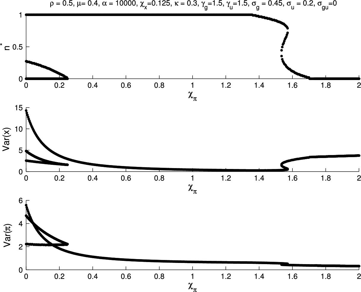
The bottom two panels plot the variances of the output gap and inflation within a Misspecification Equilibrium (as plotted in the top panel). The amount of economic volatility induced by a given policy rule choice depends on the particular equilibrium that agents coordinate on. Conditional on a particular type of equilibrium, more aggressive policy responses to inflation stabilizes both the output gap and inflation. However, a bifurcation can increase or reduce that volatility. Notice, in particular, that when the equilibrium bifurcates from the n=1![]() equilibrium to the Intrinsic Heterogeneity equilibrium, there is a large jump in economic volatility, especially in the output gap. This happens because Intrinsic Heterogeneity has agents using both the lower volatility demand shocks and the higher volatility supply shocks.
equilibrium to the Intrinsic Heterogeneity equilibrium, there is a large jump in economic volatility, especially in the output gap. This happens because Intrinsic Heterogeneity has agents using both the lower volatility demand shocks and the higher volatility supply shocks.
Branch and Evans (2011) also draw other policy implications from the model. In some calibrations, there exists a unique misspecification equilibrium for lower values of χπ![]() and multiple equilibria for more aggressive policy stances. Thus, a policymaker that becomes more aggressive in the policy rule can inadvertently bring the economy to coordinate on a more volatile equilibrium and there may be hysteresis effects if they, in turn, bring the reaction coefficient back down. A second implication is a bad luck shock that increases the variance and persistence of the supply shock – like the experience of the 1970's that preceded the Great Moderation, can lead to the existence of multiple equilibria and the possibility of an abrupt jump in volatility. Similar to a finding in Branch and Evans (2007) real-time learning can lead to endogenous regime-switching between high and low volatility regimes, as the result of policy hysteresis, similar to what was observed in US data with a switch into and out of the Great Moderation. A calibration exercise shows that this model does a good job matching statistics on volatility and persistence. Finally, it is shown that optimal discretionary policy leads to an expectations-based rule similar to Evans and Honkapohja (2003). The optimal policy rule then features agents coordinating on the unique low volatility equilibrium.
and multiple equilibria for more aggressive policy stances. Thus, a policymaker that becomes more aggressive in the policy rule can inadvertently bring the economy to coordinate on a more volatile equilibrium and there may be hysteresis effects if they, in turn, bring the reaction coefficient back down. A second implication is a bad luck shock that increases the variance and persistence of the supply shock – like the experience of the 1970's that preceded the Great Moderation, can lead to the existence of multiple equilibria and the possibility of an abrupt jump in volatility. Similar to a finding in Branch and Evans (2007) real-time learning can lead to endogenous regime-switching between high and low volatility regimes, as the result of policy hysteresis, similar to what was observed in US data with a switch into and out of the Great Moderation. A calibration exercise shows that this model does a good job matching statistics on volatility and persistence. Finally, it is shown that optimal discretionary policy leads to an expectations-based rule similar to Evans and Honkapohja (2003). The optimal policy rule then features agents coordinating on the unique low volatility equilibrium.
6.3 Heterogeneous Expectations and Liquidity Traps
An insight of Branch and McGough (2009) is that heterogeneous expectations can alter the determinacy properties of a model. Branch and Kukacka (2016) use this insight in a New Keynesian model where there are multiple steady-states that arise from a zero lower bound constraint on the central bank's policy rule. While this framework has been studied in many papers, see for instance Evans and Honkapohja (2005), typically the so-called liquidity trap equilibrium is unstable under learning. Here we show how both the normal equilibrium and the liquidity trap equilibrium can be stable under learning by introducing heterogeneity of the type considered throughout this chapter.
Branch and Kukacka (2016) work with a version of the New Keynesian model with heterogeneous expectations extended to include a non-zero inflation target and a Taylor rule with a lower bound:
yt=ˆEtyt+1−υ−1(it−ˉi−ˆEtπt+1+rnt)πt=βˆEtπt+1+κyt+utit=max{χπ(πt−ˉπ)+χy(yt−ˉy)+ηt,0}
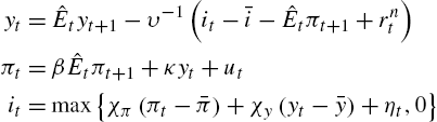
For the purposes here, assume that the exogenous shocks rn,u,η![]() are mean-zero i.i.d. In Branch and Kukacka (2016) the central bank's target ˉπ
are mean-zero i.i.d. In Branch and Kukacka (2016) the central bank's target ˉπ![]() follows a highly persistent serially correlated process that is unobservable to agents. There are two steady-states to the model. The first corresponding to the central bank's long-run inflation target ˜π=ˉπ
follows a highly persistent serially correlated process that is unobservable to agents. There are two steady-states to the model. The first corresponding to the central bank's long-run inflation target ˜π=ˉπ![]() and the corresponding steady-state output gap ˜x=ˉx≡(1−β)ˉπ/κ
and the corresponding steady-state output gap ˜x=ˉx≡(1−β)ˉπ/κ![]() . There is also an unintended “liquidity trap” steady-state with i=0
. There is also an unintended “liquidity trap” steady-state with i=0![]() and ˜π=−ˉr,˜x=−(1−β)ˉr/κ
and ˜π=−ˉr,˜x=−(1−β)ˉr/κ![]() . The paper studies the extent to which changes in that process and structural change in the supply shocks affects the basin of attraction of the liquidity trap equilibrium, i.e. the likelihood of escapes to the zero lower bound. Throughout, the model is parameterized so that around each equilibrium there is a locally unique rational expectations equilibrium.
. The paper studies the extent to which changes in that process and structural change in the supply shocks affects the basin of attraction of the liquidity trap equilibrium, i.e. the likelihood of escapes to the zero lower bound. Throughout, the model is parameterized so that around each equilibrium there is a locally unique rational expectations equilibrium.
As before, we assume that agents are distributed across two forecasting models. We assume that a fraction n of agents adopt a perceived law of motion that has the same form as the unique rational expectations equilibrium. The remaining fraction, 1−n![]() , of agents adopt an anchoring-and-adjustment rule:
, of agents adopt an anchoring-and-adjustment rule:
wt=˜w+θ(wt−1−˜w)
for some state variable w. Without loss of generality, we assume that the anchoring-and-adjustment agents know the steady-state value of interest ˜w![]() . Branch and Kukacka (2016) assume a learning process for the anchor. Plugging in expectations from these agents leads to a stacked system of equations:
. Branch and Kukacka (2016) assume a learning process for the anchor. Plugging in expectations from these agents leads to a stacked system of equations:
Xt=A+FˆE1tXt+1+BXt−1+CZt
where X′=(y,π)![]() and Z′=(rn,u,η)
and Z′=(rn,u,η)![]() , for appropriate matrices A,B,C,F
, for appropriate matrices A,B,C,F![]() .
.
The rational expectations equilibrium properties for a neighborhood of the targeted steady-state are well-known: the targeted steady-state is determinate provided that χπ![]() is sufficiently large and χy
is sufficiently large and χy![]() is not too big. Assuming ˆE1
is not too big. Assuming ˆE1![]() is a rational predictor, it is possible to follow Branch and McGough (2009) and also characterize the determinacy properties of the model near the liquidity trap steady-state:
is a rational predictor, it is possible to follow Branch and McGough (2009) and also characterize the determinacy properties of the model near the liquidity trap steady-state:
- • For θ<1
 , and n sufficiently small, there exists a unique rational expectations equilibrium in a neighborhood of the liquidity trap steady-state. For n sufficiently large, the liquidity trap steady-state exhibits order-one indeterminacy.
 - • For θ>1, and n sufficiently small, the liquidity trap steady-state exhibits order-two indeterminacy.
Thus, the case of a model where θ<1![]() and n<1
and n<1![]() is sufficiently small, then the liquidity trap is determinate. When n=1
is sufficiently small, then the liquidity trap is determinate. When n=1![]() , i.e. under rational expectations, the liquidity trap equilibrium is indeterminate and, as a result, it is typically unstable under learning. Thus, the interesting case is θ<1
, i.e. under rational expectations, the liquidity trap equilibrium is indeterminate and, as a result, it is typically unstable under learning. Thus, the interesting case is θ<1![]() and a sufficient number of adaptive agents so that the liquidity trap equilibrium is determinate.
and a sufficient number of adaptive agents so that the liquidity trap equilibrium is determinate.
In the neighborhood of a determinate steady-state, there exists a unique rational expectations equilibrium of the form
Xt=a+bXt−1+noise
Rather than rational expectations, a fraction n adopt a predictor that has a VAR(1) form:
ˆE1tXt+1=a(1+b)+b2Xt−1
Plugging in these beliefs, leads to an actual law of motion:
Xt=A+F(I+b)a+(Fb2+B)Xt−1+CZt
Notice that because of the heterogeneity, the actual law of motion depends on lags of the endogenous state variables. Thus, agents of type-1 beliefs have a properly specified statistical model of the economy. The T-map coefficients of the perceived law of motion into the actual law of motion are:
a→A+F(I+b)ab→Fb2+b
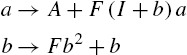
A rational expectations equilibrium, i.e. a heterogeneous expectations equilibrium, arises when the coefficients (a,b)![]() are fixed points of the T-map. Moreover, the T-map contains useful information about the stability of the REE under adaptive learning. For reasonable learning algorithms, such as recursive least-squares, asymptotic stability is governed by the “E-stability” o.d.e.:
are fixed points of the T-map. Moreover, the T-map contains useful information about the stability of the REE under adaptive learning. For reasonable learning algorithms, such as recursive least-squares, asymptotic stability is governed by the “E-stability” o.d.e.:
d(a,b)′dτ=T(a,b)−(a,b)′
An REE is a resting point of the E-stability o.d.e. Moreover, the E-stability principle holds that if an REE is a stable resting point of the E-stability o.d.e. then it will be stable under adaptive learning. Thus, it suffices to check whether the unique REE is E-stable. Branch and Kukacka (2016) provide a detailed analysis that shows under reasonable calibrations of the model, the liquidity trap equilibrium is stable under learning. For example, with the parameterization, n=0.7,θ=0.2,β=0.99,υ=0.167,κ=0.15![]() the liquidity trap equilibrium is determinate and E-stable.
the liquidity trap equilibrium is determinate and E-stable.
The stability of the liquidity trap arises because of the heterogeneity in expectations. The role that heterogeneity plays in altering the dynamic properties of otherwise standard models can help explain many features of the data. In Branch and Kukacka (2016) it can explain how an economy can endogenously collapse to a liquidity trap, and then remain in the liquidity trap for a long period of time. Most models of learning and heterogeneous expectations find that either the economy will eventually converge back to the targeted steady-state on its own, or else the time paths will feature deflationary spirals. Neither feature is observed in data for economies that have been at zero nominal interest rates for long stretches of time.
6.4 Heterogeneity and Business Cycles Amplification
Branch and McGough (2011) study the implications for business cycle dynamics in a real business cycle (RBC) model with extrinsically heterogeneous expectations. It is well-known (see Cogley and Nason, 1995) that real business cycle models have very little internal propagation as output inherits most of its time series properties from the assumed exogenous process for technology. Branch and McGough (2011) show that a real business cycle model extended to include heterogeneous expectations can have output effects that significantly amplify technology shocks.11
In the model, households choose consumption, labor supply and savings. A competitive rental market for capital exists that channels savings into capital accumulation which is then rented to firms in a competitive market. All production takes place with a constant returns to scale production technology that combines consumption and labor. Branch and McGough (2011) assume that agents are identical except for their expectations operator.
Households are, further, assumed to be anticipated utility maximizers who choose their consumption, labor and savings plans in order to satisfy an N-step Euler equation, found by log-linearizing the Euler and iterating N periods ahead. Specifically, the household's first-order conditions for an agent of expectations-type τ are:
(26) cτt=ˆEτtcτt+N−βrN∑i=1ˆEτtrt+icτt+ηhlhτt=wt
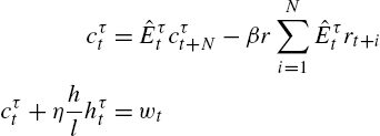
and the household's flow budget constraint. The first equation in (26) is the N-step Euler equation. Thus, (26) is a form of finite-horizon learning, which was generalized and studied in Branch et al. (2012).
Branch and McGough (2011) specify expectations as a mixture of rational expectations and forecasts that are generated from a parsimonious forecasting rule that depends linearly on the lagged capital stock. The boundedly rational forecasts are underparameterized because in the RBC model the state variables are the capital stock and the real interest rate. Thus, Branch and McGough (2011) focus on a restricted perceptions equilibrium with the agents who adopt parsimonious forecasting models choosing the parameters of their model as optimal within the restricted class. Branch and McGough (2011) then study the effect that heterogeneity, and in particular the planning horizon N, has on the propagation of technology shocks to output.
Fig. 14 presents a key result from Branch and McGough (2011). In this figure an impulse response to a technology is plotted for various parameterizations of the degree to which there is extrinsic heterogeneity. The parameter n is the fraction of households with rational expectations implying that 1−n![]() is the fraction with restricted perceptions. The model was calibrated using standard parameters, and the impulse response was computed within a restricted perceptions equilibrium holding the planning horizon fixed at N=20
is the fraction with restricted perceptions. The model was calibrated using standard parameters, and the impulse response was computed within a restricted perceptions equilibrium holding the planning horizon fixed at N=20![]() , i.e. households have a planning horizon of five years. The dashed line is the impulse response under homogeneous rational expectations. Then the solid lines correspond to the impulse response assuming heterogeneous expectations with each line corresponding to a fraction of rational agents, as indicated by the arrow in Fig. 14.
, i.e. households have a planning horizon of five years. The dashed line is the impulse response under homogeneous rational expectations. Then the solid lines correspond to the impulse response assuming heterogeneous expectations with each line corresponding to a fraction of rational agents, as indicated by the arrow in Fig. 14.
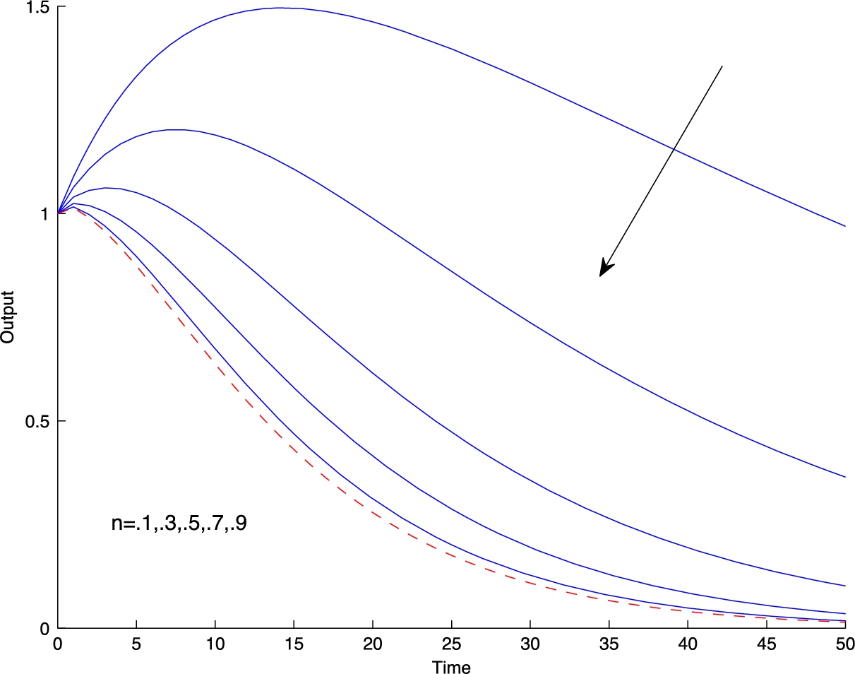
The rational expectations model features very little additional propagation and very little persistence from the shock. In contrast, the impulse response under heterogeneous expectations features a hump-shaped response to the technology shock, in line with results from structural VAR models. Notice also that as the fraction of rational agents decreases the output response to a technology shock becomes stronger and more persistent. In particular, with a value of n=0.1![]() the peak effect on output from a one standard deviation technology shock exhibits a strong hump-shaped effect with a peak response of approximately 50%. Thus, heterogeneous expectations can bring a strong propagation mechanism into a business cycle model with very little internal propagation.
the peak effect on output from a one standard deviation technology shock exhibits a strong hump-shaped effect with a peak response of approximately 50%. Thus, heterogeneous expectations can bring a strong propagation mechanism into a business cycle model with very little internal propagation.
6.5 Related Literature
Following Branch and McGough (2009) an extensive literature studies the monetary policy implications of heterogeneous expectations in New Keynesian type models. Massaro (2013) considers rationally heterogeneous expectations – and the large type limit – in a New Keynesian model with long-horizon expectations. Massaro shows that the long-horizon approach generalizes the aggregation result in Branch and McGough (2009) without requiring some of the more restrictive axioms regarding higher-order beliefs. Harrison and Taylor (2012) apply the Massaro approach of long-horizon expectations to a stochastic model and show that it does a good job explaining business cycle facts. Anufriev et al. (2013) show that the Taylor principle is not sufficient to guarantee stability in a Fisherian type model with the large-type-limit beliefs. Lines and Westerhoff (2010) develop a rationally heterogeneous expectations model in a simple textbook model of the economy. Gasteiger (2014) studies the optimal monetary policy problem in the New Keynesian with heterogeneous expectations framework. Similarly, Gasteiger (2017) illustrates the implications of heterogeneity for monetary/fiscal policy interactions in a fiscal theory of the price level environment. Di Bartolomeo et al. (2016) study the fully optimal policy problem where the social welfare function is derived assuming the existence of heterogeneous expectations in a micro-founded NK model. Finally, Hommes and Lustenhouwer (2015) and Hommes and Lustenhouwer (2016) extend the New Keynesian environment of Branch and McGough (2009) to include a zero lower bound on policy rates and where predictors are distributed around the central bank's long-run inflation target.
There is also an extensive literature that incorporates heterogeneous expectations using alternative approaches. For example, Kurz et al. (2013) develop a rational belief equilibrium in a New Keynesian model. De Grauwe (2011) uses a stylized New Keynesian model with biased heterogeneous beliefs, with the distribution evolving adaptively, to show existence of waves of optimism and pessimism. A similar framework set in an overlapping generations monetary model was developed by Brazier et al. (2008). Pfajfar (2013) develops an extension to the rationally heterogeneous expectations approach where agents decide both on their predictor and, in a second stage, whether to update their information sets. Applications of rationally heterogeneous expectations to survey data are made by Branch (2004), Branch (2007), and Pfajfar and Santoro (2010). Heterogeneity that arises from a genetic algorithm were applied to a New Keynesian model by Arifovic et al. (2013) who show that Taylor rules that would lead to indeterminacy under rational expectations can be stable with evolutionary learning. Gibbs (2017) uses forecast combination as a proxy for heterogeneous expectations in a pure currency economy. Nakagawa (2015) addresses the conditions under which monetary policy rules can ensure the expectational stability of misspecification equilibria.
Following the Great Recession and the 2007–2009 financial crisis, a number of papers have used expectations misspecification and heterogeneity to address relevant issues in the housing market and the macroeconomy. For example, Bofinger et al. (2013) incorporate heterogeneous expectations via simple heuristics in a New Keynesian model extended to include housing services and a collateral constraint. Similarly, Ascari et al. (2017) use heterogeneous expectations (chartists vs. fundamentalists) to explain the housing boom and bust in a DSGE model with a financing constraint. In a model with two sectors and labor market and goods market frictions, Branch et al. (2016) show that learning is essential to generate a housing boom and bust that leads to equilibrium unemployment rates consistent with those observed in the data over the period 1996–2010.
7 Conclusion
Heterogeneous expectations are increasingly being employed in macroeconomics. Heterogeneity in beliefs can alter the nature of trade in decentralized markets with important implications for welfare. An empirically realistic model of time-varying heterogeneous beliefs can lead to bubbles and crashes as the distribution of agents across forward- and backward-looking expectations evolves along with the state variables in DSGE and asset-pricing models that exhibit strong expectational feedback effects. Heterogeneity of beliefs also has implications for the set of equilibria and for the design of monetary policy rules that stabilize the economy near a central bank's objectives.
There are also substantive modeling issues associated with incorporating heterogeneous expectations into DSGE models. Section 2 of the chapter presented several frameworks for modeling bounded optimality. That is, we considered a variety of behavioral primitives that describe the decision-making of agents with boundedly rational expectations. We considered two alternatives based on a variational principle, shadow-price learning and Euler equation learning. We also considered a formulation where long horizon – both finitely and infinitely long – expectations matter for decision-making. We showed the implications of these behavioral rules for aggregating the decision rules of individual agents who hold heterogeneous expectations. Finally, we demonstrated two ways in which heterogeneous expectations can arise endogenously as an equilibrium object.
Despite considerable experimental and empirical evidence in favor of heterogeneous expectations, the DSGE literature incorporating heterogeneous beliefs is still in its infancy. This chapter provided an overview of many of the key contributions, but there is still much work to be done. Especially in models with market frictions, such as labor and money search models, the welfare and policy implications are starkly different from what arises under homogeneous, rational expectations. There is a need for more research on establishing the terms of trade in decentralized markets between buyers and sellers who hold different beliefs, a situation that describes most economic transactions.