3.1 Balance Sheet Composition

When developing a model of a financial system, it is useful to distinguish between two types of agents which we refer to as “active” and “passive” agents. Active agents are the objects of interest and their internal state and interactions are carefully modeled. Passive agents represent parts of the financial system that interact with active agents but are not the focus of the model, and are therefore typically represented by simple stochastic processes. For the remainder of this review, consider a financial system that consists of a set $\mathcal{B}$ of active leveraged investors and a set of passive agents which will remain unspecified for now. We are particularly interested in systemic risk that is driven by borrowing, and thus we focus on agents that use leverage (defined as purchasing assets with borrowed funds). However, the setup below is sufficiently general to accommodate unleveraged investors as a special case with leverage equal to one.

Leveraged investors need not be homogeneous and may differ, among other aspects, in their balance sheet composition, strategies or counterparties. In practice, a leveraged investor might be a bank or a leveraged hedge fund and other active investors might include unleveraged mutual funds. Passive agents could be depositors, noise traders, fund investors that generate investment flows or banks that lend to hedge funds. The choice of active vs. passive investors of course varies from model to model.

The balance sheet of an investor $i\in \mathcal{B}$ is composed of assets $A_i$, liabilities $L_i$, and equity $E_i$, such that $A_i=L_i+E_i$. The investor's leverage is simply the ratio of assets to equity ${\lambda }_i=A_i/E_i$. It is useful to decompose the investor's assets into three classes: bilateral contracts $A_i^B$ between investors, such as loans or derivative exposures; traded securities $A_i^S$, such as stocks; and external assets $A_i^R$, whose value is assumed exogenous. Throughout this review, we assume that the value $A_i^S$ of traded securities is marked to market.⁶ That is, the value of a traded security on the investor's balance sheet will be determined by its current market price. Of course we must have that $A_i=A_i^B+A_i^S+A_i^R$. Each asset class can be further decomposed into individual loan contracts, stock holdings and so on.

The investor's liabilities can be decomposed in a similar fashion. For now, let us decompose the investor's liabilities simply into bilateral contracts $L_i^B$ between investors, such as loans or derivative exposures, and external liabilities $L_i^R$ which can be assumed exogenous. In the case of a bank, these external liabilities might be deposits. Again we must have that $L_i=L_i^B+L_i^R$, and bilateral liabilities can be further decomposed into individual bilateral contracts. Bilateral assets and liabilities might be secured, such as repurchase agreements, or unsecured such as interbank loans. Naturally, bilateral liabilities are just the flip side of bilateral assets such that summing over all investors we must have ${\sum }_i{A}_i^B={\sum }_i{L}_i^B$.

3.2 Balance Sheet Dynamics

Of all the factors that affect the dynamics of the investors' balance sheets, three are of particular importance for financial stability: leverage, liquidity, and interconnectedness. Below, we discuss each factor in turn.

Leverage: Leverage amplifies returns, both positive and negative. Therefore, investors typically face a leverage constraint to limit the investors' risk.⁷ However, at the level of the financial system, binding leverage constraints can lead to substantial instabilities. On short time scales, a leveraged investor may be forced to sell into falling markets when she exceeds her leverage constraint. Her sales will in turn depress prices further as we explain in the next paragraph on market liquidity. Leverage constraints can thus lead to an unstable feedback loop between falling prices and forced sales. On longer time scales dynamic leverage constraints that depend on backward looking risk estimates can lead to entirely endogenous volatility – so called leverage cycles.⁸

Liquidity: Broadly speaking, one can distinguish between two types of liquidity: market liquidity and funding liquidity.

Market liquidity can be understood as the inverse to price impact. When market liquidity is high, the market can absorb large sell orders without large changes in the price. If markets were perfectly liquid it would always be possible to sell assets without affecting prices and most forms of systemic risk would not exist.⁹ Leverage is dangerous both because it directly increases risk, amplifying gains and losses proportionally, but also because the market impact of liquidating a portfolio to achieve a certain leverage increases with leverage. This point was stressed by Caccioli et al. (2012a), who showed how, due to her own market impact, an investor with a large leveraged position can easily drive herself bankrupt by liquidating her position. They showed that this can be a serious problem even under normal market conditions, and recommended taking market impact into account when valuing portfolios in order to reduce this problem. The problem can become even worse if investors are forced to sell too quickly, inducing fire sales in which a market is overloaded with sell orders, causing a dramatic decrease in liquidity for sellers.¹⁰ Fire sales can be induced when investors hit leverage constraints, forcing them to sell, which in turn causes leverage constraints to be more strongly broken, inducing more selling.

Funding liquidity refers to the ease with which investors can borrow to fund their balance sheets. When funding liquidity is high, investors can easily roll over their existing liabilities by borrowing again, or even expand their balance sheets. In times of crises, funding liquidity can drop dramatically. If investors rely on short term liabilities they may be forced to liquidate a large part of their assets to pay back their liabilities. This forced sale can trigger fire sales by other investors.

Interconnectedness: Investors are connected via their balance sheets and so are not isolated agents. Connections can result from direct exposures due to bilateral loan contracts, or from indirect exposures due to investments into the same assets. Interconnectedness together with feedback loops resulting from binding leverage constraints and endogenous liquidity can lead to financial contagion. In analogy to epidemiology, financial contagion refers to the process by which “distress” may spread from one investor to another, where distress can be broadly understood as an investor becoming uncomfortably close to insolvency or illiquidity. Typically financial contagion arises when, via some mechanism or channel, a distressed investor's actions negatively affect some subset of other investors. This subset of investors is said to be connected to the distressed investor. A simple example of such connections are the bilateral liabilities between investors. Taken together, the set of all such connections form a network over which financial contagion can spread. For an in-depth review of financial networks see Iori and Mantegna (2018).

The aim of the subsequent sections is to introduce the reader to a number of models that tackle the effect of leverage, liquidity and interconnectedness on financial stability in isolation. These models then form the building blocks of more comprehensive models discussed in Section 6. Below, in Section 4, we first focus on the potentially destabilizing effects of leverage as they form the basis of fire sale models discussed later, and because they are thought to have contributed to the build up of risk prior to the great financial crisis. In Section 5 we then proceed to models of financial contagion as they form the scientific bedrock of the stress testing models that will be discussed in Section 6 and beyond. While liquidity is of great importance, we will only discuss it implicitly in Sections 4 and 5, rather than dedicating a separate section to it. This is because, unfortunately, there are currently only few dedicated models on this topic, see Bookstaber and Paddrik (2015) for an example. We will not be able to provide a complete overview of the agent-based modeling literature devoted to various aspects of financial stability. Important topics that we will not be able to discuss include the role of heterogeneous expectations or time scales in the dynamics of financial markets, see for example Hommes (2006), LeBaron (2006) for early surveys, and Dieci and He (2018) for a recent overview.

4.1 Leverage and Balance Sheet Mechanics

Many financial institutions borrow and invest the borrowed funds into risky assets. Three simple properties of leverage are worth noting at this point. First, ceteris paribus, leverage determines the size of the investor's balance sheet. Second, leverage boosts asset returns. Third, leverage increases when the investor incurs losses, again ceteris paribus. In the following, we discuss each property in turn. For a fixed amount of equity, an investor can only increase the size of its balance sheet by increasing its leverage. Further, it is easy to show that, if $r_t$ is the asset return, the equity return is $u_t=\lambda r_t$, where, as above, λ is the investor's leverage. In good times, leverage thus allows an investor to boost its return. In bad times however, even small negative asset returns can drive the investor into bankruptcy provided leverage is sufficiently high. Given the potential risks associated with high leverage, an investor typically faces a leverage limit which may be imposed by a regulator, as is the case for banks, or by creditors via a haircut¹¹ on collateralized debt. Finally, why does leverage increase when the investor incurs losses? Suppose the investor holds S units of a risky asset at price p such that $A=Sp$. Holding the investor's liabilities fixed, it is easy to see that $\lambda >1$ implies $\partial \lambda /\partial p<0$. In other words, whenever an investor is leveraged ($\lambda >1$), a decrease (increase) in asset prices leads to an increase (decrease) in its leverage.

In what follows, we discuss how these three properties of leverage, in combination with reasonable assumptions about investor behavior, can lead to financial instability. We begin by discussing how leverage constraints can force investors to sell into falling markets even if they would prefer to buy in the absence of leverage constraints. We then show how a leverage constraint based on a backward looking estimator of market risk can lead to endogenous volatility and leverage cycles.

4.2 Leverage Constraints and Margin Calls

Consider again the simple investor discussed above. Suppose the investor faces a leverage constraint $\bar{\lambda }$ and has leverage ${\lambda }_{t-1}<\bar{\lambda }$.¹² The investor has to decide on an action at time $t-1$ to ensure that it does not violate its leverage constraint at time t. Suppose the investor expects the price of the risky asset to drop sufficiently from one period to the next, such that its leverage is pushed beyond its limit, i.e. ${\lambda }_t>\bar{\lambda }$. In this situation the investor has two options to decrease its leverage: raise equity or reduce its assets (or some combination of the two). Raising equity can be time consuming or even impossible during a financial crisis. Therefore, if the leverage constraint has to be satisfied quickly or if new equity is not available and no assets are maturing in the next period, the investor has to sell at least $\mathrm{\Delta }{A}_{t-1}=\text{max}\{0,({\mathbb{E}}_{t-1}[{\lambda }_t]-\bar{\lambda }){\mathbb{E}}_{t-1}[E_t]\}$ of its assets to satisfy its leverage constraint, where ${\mathbb{E}}_t[\cdot ]$ is the conditional expectation at time t. In the following we will set ${\mathbb{E}}_t[{\lambda }_{t+1}]={\lambda }_t$ and ${\mathbb{E}}_t[E_{t+1}]=E_t$. This can be done for simplicity or because a contract forces the investor to make adjustments based on current rather than expected values. In this case we have simply $\mathrm{\Delta }{A}_t=\text{max}\{0,({\lambda }_t-\bar{\lambda })E_t\}$. If ${\lambda }_t$ exceeds the leverage limit due to a drop in prices, the investor will sell into falling markets which may lead to a feedback loop between leverage and falling prices as outlined in the previous section.

This simple mechanism has been discussed by a number of authors, see for example Gennotte and Leland (1990), Geanakoplos (2010), Thurner et al. (2012), Shleifer and Vishny (1997), Gromb and Vayanos (2002), Fostel and Geanakoplos (2008). Gorton and Metrick (2012) study the effect of haircuts on repo markets during the financial crisis empirically. Thurner et al. (2012) incorporate this mechanism in a heterogeneous agent model of leverage-constrained value investors. In the remainder of this section we will introduce their model and discuss some of the quantitative results they obtain for the effect of leverage constraints on asset returns.

Consider our set $\mathcal{B}$ of leveraged investors introduced in Section 3. Suppose that investors have no bilateral assets or liabilities and only invest into a single traded security, i.e. $A_i=A_i^S$. Furthermore, assume that the investor has access to a credit line from an unmodeled bank such that $L_i=L_i^R$. For brevity and to guide intuition, we will refer to these leveraged investors as funds for the remainder of this section. In addition to the funds, there is a representative noise trader and a representative “fund investor” that allocates capital to the funds. There is an asset of supply N with fundamental value V that is traded by the funds and the noise trader at discrete points in time $t\in \mathbb{N}$. Every period a fund i takes a long position $A_{it}={\lambda }_{it}{E}_{it}$ provided its equity satisfies $E_{it}⩾0$. The fund's leverage is given by the heuristic

${\lambda }_{it}=\text{min}\{{\beta }_i{m}_t,\bar{\lambda }\},$

where $m_t=\text{max}\{0,V-p_t\}$ is the mispricing signal and ${\beta }_i$ is the fund's aggressiveness. In other words, the fund goes long in the asset if the asset is underpriced relative to its fundamental value V. The noise trader's long position follows a transformed AR(1) process with normally distributed innovations. The price of the asset is determined by market clearing. Every period, the fund investor adjusts its capital allocation to the funds, withdrawing capital from poorly performing funds and investing into successful funds relative to an exogenous benchmark return.

Before considering the dynamics of the full model, let us briefly discuss the limit where the funds are small, i.e. $E_{it}\to 0$. In this case, in the absence of any significant effect of the funds, log price returns will be approximately iid normal due to the action of the noise trader. This serves as a benchmark. The authors then calibrate the parameters of the model such that funds are significant in size and prices may deviate substantially from fundamentals. This corresponds to a regime where arbitrage is limited as in Shleifer and Vishny (1997). The authors also assume that funds differ substantially in their aggressiveness ${\beta }_i$ but share the same leverage constraint $\bar{\lambda }$ and initial equity $E_{i0}$.

In this setting the funds' leverage and wealth dynamics can lead to a number of interesting phenomena. When the noise trader's demand drives the price below the asset's fundamental value, funds will enter the market in proportion to their aggressiveness ${\beta }_i$. Due to the built-in tendency of the price to revert to its fundamental value due to the action of the noise traders, these trades will be profitable for the funds on average and even more profitable for more aggressive funds. Hence, the equity of aggressive funds grows quicker due to a combination of profits and capital reallocation of the fund investor. Importantly, as the equity of funds grows, their influence on prices increases and the volatility of the price decreases, due to the fact that they buy into falling markets and sell into rising markets.

Aggressive funds are also more likely to leverage to their maximum. Consider an aggressive fund i that has chosen ${\lambda }_{it-1}=\bar{\lambda }$. Now suppose the price drops such that ${\lambda }_{it}>\bar{\lambda }$. In response the fund sells parts of its assets as outlined above. Thurner et al. (2012) refer to this forced selling as a margin call, as they interpret the leverage constraint as arising from a haircut on a collateralized loan. Recall that the amount the fund will sell is $\mathrm{\Delta }{A}_{it}=\text{max}\{0,({\lambda }_{it}-\bar{\lambda })E_{it}\}$, i.e. it is proportional to the fund's equity. As the aggressive fund is likely also the most wealthy fund, its selling can be expected to lead to a significant drop in prices. This drop may push other, less aggressive funds past their leverage limits. A margin spiral ensues in which more and more funds are forced to sell into falling markets. In an extreme outcome, most funds will exit or will have lost most of their equity in the price crash. As a result, their impact on prices is limited and the price is dominated by the noise trader. Thus following a margin spiral, price volatility increases due to two forces. First, it spikes due to the immediate impact of the price collapse. But then, it remains at an elevated level due to lack of value investors that push the price toward its fundamental value. These dynamics, which are illustrated in Fig. 1, reproduce some important features of financial time series in a reasonably quantitative way, in particular fat tails in the distribution of returns and clustered volatility (cf. Cont, 2001), as well as a realistic volatility dynamics profile before and after shocks (Poledna et al., 2014). These are difficult to reproduce in standard models.

One would expect these dynamics to be less drastic if funds took precautions against margin calls and stayed some $ϵ>0$ below their maximum leverage allowing them to more smoothly adjust to price shocks. However, it is important to note that a single “renegade” fund that pushes its leverage limit while all other funds remain well below it can be sufficient to cause a margin spiral.

It should be noted that the deleveraging schedule $\mathrm{\Delta }{A}_{it}$ that a fund follows can depend on how the leverage constraint is implemented. In Thurner et al. (2012), the leverage constraint results from a haircut applied to a collateralized loan, i.e. the fund obtains a short term loan from a bank, purchases the asset with the loan and its equity and then posts the asset as collateral for the loan. The haircut is equivalent to leverage and determines how much of its assets the fund can finance via borrowing. When the value of the asset drops, the bank will make a margin call as outlined above and the fund will have to sell assets immediately. However, a leverage constraint can, for example, also be imposed by a regulator. In this case, the fund may be allowed to violate the leverage constraint for a few time steps while smoothly adjusting to satisfy the constraint in later periods. Such an implementation will increase the stability of the system. Finally, the schedule $\mathrm{\Delta }{A}_{it}=\text{max}\{0,({\lambda }_{it}-\bar{\lambda })E_{it}\}$ assumes the price remains unchanged from the current to the next period. A more sophisticated fund might take its own price impact into account when determining the deleveraging schedule.

4.3 Procyclical Leverage and Leverage Cycles

In the model presented in the previous section, funds actively increase their leverage when the price falls until they reach a leverage limit. Of course, a variety of other leverage management policies are possible. In an effort to study leverage management policies, Adrian and Shin (2010) analyze how changes in leverage $\mathrm{\Delta }{\lambda }_t$ relate to changes in total assets $\mathrm{\Delta }{A}_t$ (at mark-to-market prices) during the period 1963–2006 for three types of investors: households, commercial banks and security broker dealers (such as Goldman Sachs). Below we focus on households on one extreme and broker dealers on the other.

For households and broker-dealers the authors find a distinct correlation between leverage and asset changes, see Fig. 2. For households, changes in leverage are negatively correlated to changes in assets: $\text{Corr}(\mathrm{\Delta }{\lambda }_t,\mathrm{\Delta }{A}_t)<0$. For broker dealers they find a positive correlation $\text{Corr}(\mathrm{\Delta }{\lambda }_t,\mathrm{\Delta }{A}_t)>0$. This points toward at least two distinct leverage management policies.

Households appear to be passive investors since leverage decreases when assets appreciate, ceteris paribus. Broker-dealers however, appear to follow a state-contingent target leverage which they try to reach through balance sheet adjustments. To see this, suppose an investor has a leverage target which is high in good times and low in bad times. Let us say that good times are identified by increasing asset prices while bad times are identified by falling asset prices (there are other ways of identifying the state of the world as we will discuss below). In this case, in response to an increase (decrease) in the price of the asset, the investor will increase (decrease) its target leverage and adjust its balance sheet accordingly. Importantly, the leverage adjustment often occurs via debt and asset adjustment rather than equity adjustment. Adrian and Shin (2010) call this a procyclical leverage policy. With such a leverage policy we expect $\text{Corr}(\mathrm{\Delta }{\lambda }_t,\mathrm{\Delta }{A}_t)>0$. Hence, it appears that broker-dealers follow a procyclical leverage policy.

A procyclical leverage policy could arise if the broker-dealers face a time varying leverage constraint and choose to leverage maximally. In fact, Adrian and Shin (2010), Danıelsson et al. (2004), and others show that a time varying leverage constraint arises when the investor faces a Value-at-Risk (VaR) constraint as was required under the Basel II regulatory framework. As we will show below, the effect of a VaR constraint is that the investor faces a leverage constraint that is inversely proportional to market risk. Thus, when market risk is high (low), the leverage constraint is low (high). In this setting the level of risk identifies the state of the world: in good times risk is low, while in bad times risk is high.

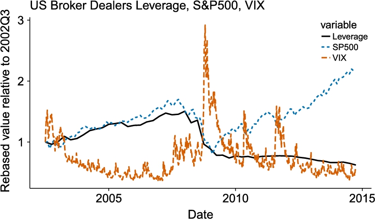
In summary, two leverage management policies are borne out by the data: passive leverage and procyclical target leverage. The type of leverage management policy used by the investor can have significant implications for financial stability. Indeed, at least anecdotally, the time series of broker-dealer leverage,¹³ perceived risk (as measured by the VIX) and asset prices (as measured by the S&P500) in Fig. 3 suggests a relationship between these three variables that is potentially induced by the dealers' procyclical leverage policy. In the following, we will introduce a model developed by Aymanns and Farmer (2015) that links leverage, perceived risk and asset prices in order to illustrate the effect of procyclical leverage and VaR constraints on the dynamics of asset prices.

Consider again our set $\mathcal{B}$ of leveraged investors (banks for short) and a representative noise trader. As above, we assume that there are no bilateral assets or liabilities. There is a risk free asset (cash) and a set $\mathcal{A}$ of risky assets that are traded by banks and the noise trader at discrete points in time $t\in \mathbb{N}$. At the beginning of every period, the banks and the noise trader determine their demand for the assets. For this, each bank i picks a vector ${\mathbf{w}}_{it}$ of portfolio weights and is assigned a target leverage ${\bar{\lambda }}_{it}$. The noise trader is not leveraged and therefore only picks a vector ${\mathbf{v}}_t$ of portfolio weights. Once the agent's demand functions have been fixed, the markets for the risky assets clear which fixes prices. Given the new prices, banks choose their next period's balance sheet adjustment (buying or selling of assets) in order to hit their target leverage. We refer the reader to Aymanns and Farmer (2015) for a detailed description of the model.

As mentioned above, banks are subject to a Value-at-Risk constraint.¹⁴ Here, a bank's VaR is the loss in market value of its portfolio over one period that is exceeded with probability $1-a$, where a is the associated confidence level. The VaR constraint then requires that bank holds equity to cover these losses, i.e. $E_{it}⩾{\text{VaR}}_{it}(a)$. We approximate the Value-at-Risk by ${\text{VaR}}_{it}={\sigma }_{it}{A}_{it}/\alpha$, where ${\sigma }_{it}$ is the estimated portfolio variance of bank i and α is a parameter. This relation becomes exact for normal asset returns and an appropriately chosen α. Rearranging the VaR constraint yields the bank's leverage constraint ${\bar{\lambda }}_{it}=\alpha /{\sigma }_{it}$. We assume that the bank chooses to be maximally leveraged, e.g. for profit motives. The leverage constraint is therefore equivalent to the target leverage we discussed above. To evaluate their VaR, banks compute their portfolio variance as an exponentially weighted moving average of past log returns.

Let us briefly discuss the implications of this set up. As mentioned at the outset of this section, banks follow a procyclical leverage policy. In particular, the banks' VaR constraint, together with its choice to be maximally leveraged at all times, imply a target leverage that is inversely proportional to the banks' perceived risk as measured by an exponentially weighted moving average of past squared returns. Why is such a leverage policy procyclical? Suppose a random drop in an asset's price causes an increase in the level of perceived risk of bank i. As a result the bank's target leverage will decrease (while its actual leverage simultaneously increases) and it will have to sell some of its assets, similar to the funds in the previous section.¹⁵ The banks selling may lead to a further drop in prices and a further increase in perceived risk. In other words, the bank's leverage policy together with its perception of risk can lead to an unstable feedback loop. It is in this sense that the leverage policy is procyclical.

Banks in this model have a very simple, yet realistic, method of computing perceived (or expected) risk. Similar backward looking methods are well established in practice, see for example Andersen et al. (2006). It is important to note that perceived risk ${\sigma }_{it}$ and realized volatility over the next time step can be very different. Since banks have only bounded rationality and follow a simple backward looking rule in this model, their expectations about volatility are not necessarily correct on average and tend to lag behind realizations.

Let us now consider the dynamics of the model in more detail. In Fig. 4 we show two simulation paths (with the same random seed) of the price of a single risky asset for two leverage policy rules. In the top panel, banks behave like the households in Adrian and Shin (2010) – they are passive and do not adjust their leverage to changes in asset prices or perceived risk. In the bottom panel, banks follow the procyclical leverage policy outlined above. The difference between the two price paths is striking. In the case of passive banks, the price follows what appears to be a simple mean reverting random walk. However, when banks follow the procyclical leverage policy, the price trajectory shows stochastic, irregular cycles with a period of roughly 100 time steps. These complex, endogenous dynamics are the result of the unstable feedback loop outlined above.

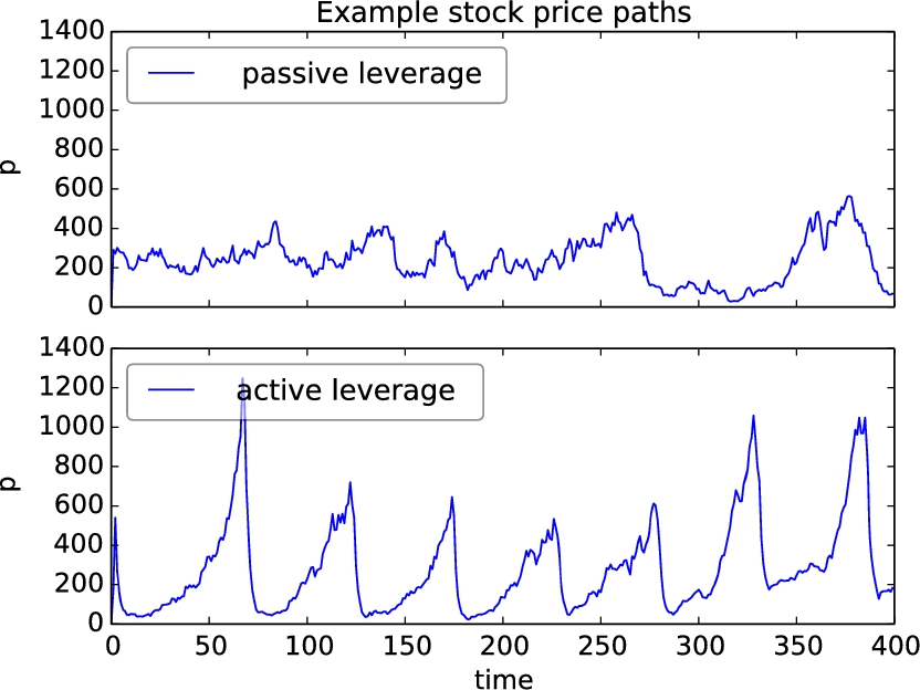
Aymanns and Farmer (2015) refer to these cycles as leverage cycles. Leverage cycles are an example of endogenous volatility – volatility that arises not because of the arrival of exogenous information but due to the endogenous dynamics of the agents in the financial system. To better understand these dynamics, consider the state of the system just after a crash has occurred, e.g. at time $t\approx 80$. Following the crash, banks' perceived risk is high, their leverage is low and prices are stable. Over time, perceived risk declines and banks increase their leverage. As they increase their leverage, they buy more of the risky assets and push up their prices. At some point leverage is sufficiently high and perceived risk sufficiently low, so that a relatively small drop of the price of an asset leads to large downward correction in leverage. A crash follows and prices fall until the noise trader's action stops the crash and the cycle begins anew. Naturally, these dynamics depend on the choice of parameters. In particular, when the banks are small relative to the noise trader, banks' trading has no significant impact on asset prices and leverage cycles do not occur. For a detailed discussion of the sensitivity of the results to parameters see Aymanns and Farmer (2015), and for a more realistic model that is better calibrated to the data, see Aymanns et al. (2016).

These results show that simple behavioral rules, grounded in empirical evidence of bank behavior (Adrian and Shin, 2010; Andersen et al., 2006), can lead to remarkable and unexpected dynamics which bear some resemblance to the run up to and crash following the 2008 financial crises. The results originate from the agents' bounded rationality and their reliance on past returns to estimate their Value-at-Risk. These features would be absent in a traditional economic models in which agents are fully rational. Indeed, rational models rarely display the dynamic instabilities that Aymanns and Farmer (2015) observe. If we believe that real economic actors are rarely fully rational, we should take note of this result. Of course, the agents in this model are really quite dumb. For example, they do not adjust to the strong cyclical pattern in the time series. However, they also live in an economy that is significantly simpler than the real world. Thus, their level of rationality in relation to the complexity of the world they inhabit might not be too far off from real economic agents' level of rationality.

The model discussed above can also yield insights for policy makers on how bank risk management might be modified in order to mitigate the effects of the leverage cycle. Aymanns et al. (2016) present a reduced form version of the model outlined above in order to investigate the implications of alternative leverage policies on financial stability. They show that, depending on the size of the banking sector and the properties of the exogenous volatility process, either a constant leverage policy or a Value-at-Risk based leverage policy is optimal from the perspective of a social planner. This finding lends support to the use of macroprudential leverage ratios as discussed in ESRB (2015). The authors also show that the timescale for the bubbles and crashes observed in the model is around 10–15 years, roughly corresponding to the run-up to the 2008 crash. Another important insight from Aymanns et al. (2016) is that the time scale on which investors need to achieve their leverage constraint plays a crucial role in the stability of the financial system: slower adjustment toward the constraint (corresponding to more slackness) increases stability.

The effect of leverage targeting on asset price dynamics has also been studied by other others in the multi-asset case. For example, Capponi and Larsson (2015) show that the deleveraging of banks may amplify asset return shocks and lead to large fluctuations in realized returns which in turn can cause spillover effects between different assets.

5.1 Financial Linkages and Channels of Contagion

A channel of contagion is a mechanism by which distress can spread from one financial institution to another.¹⁶ Often the channel of contagion is such that distress can only spread from one institution to a subset of all institutions in the system. These susceptible institutions are said to be linked to the stressed institution. The set of all links then forms a financial network associated with the channel of contagion.¹⁷ Depending on the channel, links in this network may arise directly from bilateral contracts between banks, such as loans, or indirectly via the markets in which the banks operate. In the literature, one typically distinguishes between three key channels of contagion: counterparty loss, overlapping portfolios, and funding liquidity contagion.¹⁸ Counterparty loss and overlapping portfolio contagion affect the value of the assets on the investors' balance sheet while funding liquidity contagion affects the availability of funding for the investors' balance sheets. In the following we will first introduce the investor's balance sheet relevant for this section. We will then give a brief overview of the channels of contagion before discussing each in more detail.

Balance sheet: Throughout this chapter we will consider a set $\mathcal{B}$ of leveraged investors (banks for short) whose assets can be decomposed into three classes: bilateral interbank contracts $A_i^B$, traded securities $A_i^S$ that are marked to market and external, unmodeled assets $A_i^R$. Furthermore bank liabilities can be decomposed into bilateral interbank contracts $L_i^B$, and external, unmodeled liabilities $L_i^R$ such that $L_i=L_i^B+L_i^R$. Note that bilateral interbank contracts need not be loans, they can also be derivative contracts for example. For simplicity however, we will think of bilateral interbank contracts as loans for the remainder of this section.

Counterparty loss: Suppose bank i has lent an amount C to bank j such that $A_i^B=L_j^B=C$. Now suppose the value of bank j's external assets $A_j^R$ drops due to an exogenous shock. As a result the probability of default of bank j is likely to increase, which will affect the value of the claim $A_i^B$ that bank i holds on bank j. If bank i's interbank assets are marked to market, a change in bank j's probability of default will affect the market value of $A_i^B$. In the worst case, if bank j defaults, bank i will only recover some fraction $r⩽1$ of its initial claim $A_i^B$. If the loss of bank i exceeds its equity, i.e. $(1-r)A_i^B>E_i$, bank i will default as well.¹⁹ Now, how can this lead to financial contagion? To elaborate on the above stylized example, suppose that bank i in turn borrowed an amount C from another bank k such that $A_k^B=L_i^B=C$.²⁰ In this scenario, it can be plausibly argued that an increase in the probability of default of j increases the probability of default of i which in turn increases the probability of default of k. If all banks mark their books to market, an initial shock to j can therefore end up affecting the value of the claim that bank k holds on bank i. Again, in the extreme scenario, the default of bank j may cause bank i to default which may cause bank k to default. This is the essence of counterparty loss contagion. Naturally, in a real financial system the structure of interbank liabilities will be much more complex than in the stylized example outlined above. However, the conceptual insights carry over: the financial network associated with the counterparty loss contagion channel is the network induced by the set of interbank liabilities.

Overlapping portfolios: The overlapping portfolio channel is slightly more subtle. Suppose bank i and bank j have both invested an amount C in the same security l such that $A_{il}^S=A_{jl}^S=C$, where we have introduced the additional index to reference the security.²¹ Now, suppose the value of bank j's external assets $A_j^R$ drops due to some exogenous shock. How will bank j respond to this loss? In the extreme case, when the exogenous shock causes bank j's bankruptcy ($E_i<0$), the bank will liquidate its entire investment in the security in a fire sale. However, even if the bank does not go bankrupt, it may wish to liquidate some of its investment. This can occur for example when the bank faces a leverage constraint as discussed in Section 4. Bank j's selling is likely to have price impact. As a result, the market value of $A_{il}^S$ will fall. If bank i also faces a leverage constraint, or even goes bankrupt following the fall in prices, it will liquidate part of its securities portfolio in response. How will this lead to contagion? Suppose that bank i also has invested an amount C into another security m and that another bank k has also invested into the same security, such that $A_{im}^S=A_{km}^S=C$. If bank i liquidates across its entire portfolio, it will sell some of security m following a fall in the price of security l. The resulting price impact will then affect the balance sheet of bank k which was not connected to bank j via an interbank contract or a shared security. This is the essence of overlapping portfolio contagion. Banks are linked by the securities that they co-own and the fact that they liquidate with market impact across their entire portfolios. Empirical evidence from the 2007 Quant meltdown for this contagion channel has been provided in Khandani and Lo (2011).

Funding liquidity contagion often occurs when a lender is stressed, and so often occurs in conjunction with overlapping portfolio contagion and counterparty loss contagion. To see this, let us reconsider the scenario we discussed for counterparty loss contagion. Suppose bank i has lent an amount C to bank j such that $A_i^B=L_j^B=C$. As before, suppose the value of bank j's external assets $A_j^R$ drops due to some exogenous shock and as a result, the probability of default of bank j increases. Now, suppose that every T periods bank i can decide whether to roll over its loan to bank j. Further assume that bank i is bank j's only source of interbank funding and $L_j^R$ is fixed. Given bank j's increased default probability, bank i may choose not to roll over the loan at the next opportunity. Ignoring interest payments, if bank i does not roll over the loan, bank j will have to deliver an amount C to bank i. In the simplest case, bank j may choose not to roll over its own loans to other banks which in turn may decide against rolling over their loans. This is the essence of funding liquidity contagion. As for counterparty loss contagion, the associated financial network is induced by the set of interbank loans. Empirical evidence on the fragility of funding markets during the past financial crisis has been provided for example by Afonso et al. (2011) and Iyer and Peydro (2011). In a further complication, bank j may also choose to liquidate part of its securities portfolio in order to pay back its loan. Funding liquidity contagion can therefore lead to fire sales and overlapping portfolio contagion and vice versa. This interdependence of contagion channels makes the funding liquidity and overlapping portfolio contagion processes the most challenging from a modeling perspective.

In the remainder of this section, we will discuss models for counterparty loss, overlapping portfolio and funding liquidity contagion, as well as models for the interaction of all three contagion channels.

5.2 Counterparty Loss Contagion

Let P denote the matrix of nominal interbank liabilities such that banks hold interbank assets $A_i^B={\sum }_j{P}_{ij}^T$, where T denotes the matrix transpose. In addition, banks hold external assets $A_i^R$ which can be liquidated at no cost. Banks have interbank liabilities $L_i^B={\sum }_j{P}_{ij}$ only. Assume all interbank liabilities mature at the same time and have the same seniority. We further assume that all banks are solvent initially. There is only one time period. At the end of that period all liabilities mature, external assets are liquidated and banks pay back their loans if possible. Now suppose banks are subject to a shock $s_i⩾0$ to the value of their external assets such that ${\hat{A}}_i^R=A_i^R-s_i$. Given an exogenous shock, we can ask a number of questions. First, which loan payments are feasible given the exogenous shock? Second, which banks will default on their liabilities? And finally, how do the answers to the first two questions depend on the structure of the interbank liabilities P? There is a large literature that studies counterparty loss contagion in a set up similar to the above, including Eisenberg and Noe (2001), Gai and Kapadia (2010), May and Arinaminpathy (2010), Elliott et al. (2014), Acemoglu et al. (2015), Battiston et al. (2012), Amini et al. (2016), and Capponi et al. (2015). In the following, we will briefly introduce the seminal contribution by Eisenberg and Noe (2001), who provide a solution to the first two questions. We will then consider a number of extensions of Eisenberg and Noe (2001) and alternative approaches to addressing the above questions.

Define the relative nominal interbank liabilities matrix as ${\mathrm{\Pi }}_{ij}=P_{ij}/L_i^B$ for $L_i^B>0$ and ${\mathrm{\Pi }}_{ij}=0$ otherwise. The relative liabilities matrix corresponds to the adjacency matrix of the weighted, directed network $\mathcal{G}$ of interbank liabilities. Let $\mathbf{p}=(p_1,\dots ,p_N)$ denote the vector of total payments made by the banks when their liabilities mature, where $N=|\mathcal{B}|$. Naturally, a bank pays at most what it owes in total, i.e. $p_i⩽L_i^B$. However, it may default and pay less if the value of its external assets plus the payments it receives from its debtors is less than what it owes. The individual payments that bank i makes are given by ${\mathrm{\Pi }}_{ij}{p}_i$ since by assumption all liabilities have equal seniority. The vector of payments, also known as the clearing vector, that satisfies these constraints is the solution to the following fixed point equation

(1) $p_i=\text{min}\{L_i^B,{\hat{A}}_i^R+\sum _j{\mathrm{\Pi }}_{ij}^T{p}_j\}.$

Eisenberg and Noe (2001) show that such a fixed point always exists. In addition, if within each strongly connected component of $\mathcal{G}$ there exists at least one bank with ${\hat{A}}_i^R>0$, Eisenberg and Noe (2001) show that the fixed point is unique.²² In other words, there exists a unique way in which losses incurred due to the adverse shock $\{s_i\}$ are distributed in the financial system via the interbank liabilities matrix. The clearing vector and the set of defaulting banks can be found easily numerically by iterating the fixed point map in Eq. (1). As the map is iterated, more and more banks may default, resulting in a default cascade propagating through the financial network.

It is important to note that in this setup losses are only redistributed and the system is conservative – contagion acts as a distribution mechanism but does not, in the aggregate, lead to any further losses to bank shareholders beyond the initial shock. To see this, define the equity of bank i prior to the exogenous shock as $E_i=A_i^B+A_i^R-L_i^B$ and after the exogenous shock as ${\hat{E}}_i={\hat{A}}_i^B(\mathbf{p})+A_i^R-s_i-{\hat{L}}_i^B(\mathbf{p})$. Note that post-shock both bank i's assets and liabilities depend on the clearing vector p. Taking the difference and summing over all banks we obtain ${\sum }_i{E}_i-{\hat{E}}_i={\sum }_i{A}_i^R-(A_i^R-s_i)={\sum }_i{s}_i$ since ${\sum }_i{A}_i^B={\sum }_i{L}_i^B$ and ${\sum }_i{\hat{A}}_i^B(\mathbf{p})={\sum }_i{\hat{L}}_i^B(\mathbf{p})$. Also note that, while bank shareholder losses are not amplified, losses to the total value of bank assets are amplified due to indirect losses, i.e. losses not stemming from the initial exogenous shock but due to revaluation of interbank loans. This can be seen by taking the difference between pre- and post-shock total assets in the system. The total pre-shock assets of bank i are $A_i=A_i^B+A_i^R$ and its total post-shock assets are ${\hat{A}}_i={\hat{A}}_i^B(\mathbf{p})+A_i^R-s_i$, then ${\sum }_i{A}_i-{\hat{A}}_i={\sum }_i{A}_i^B-{\hat{A}}_i^B(\mathbf{p})+s_i⩾{\sum }_i{s}_i$. Some authors argue that this total asset loss can be useful measure of systemic impact of the exogenous shock, see Glasserman and Young (2015). Finally, note that the mechanism of finding a clearing vector ignores any potential frictions in the financial system and ensures that the maximal payment is made given the exogenous shocks. Several authors have argued that this is too optimistic and assume instead that once a default has occurred, some additional bankruptcy costs are incurred, see for example Rogers and Veraart (2013) and Cont et al. (2010).^23,24 In this case, aggregate bank shareholder losses may be larger than the aggregate exogenous shock. Further shortcomings of the Eisenberg and Noe model include the lack of heterogeneous seniorities or maturities and the lack of the possibility of strategic default.

The extent of the default cascade triggered by an exogenous shock depends on the structure of the financial network induced by the matrix of interbank liabilities P. One key property of the financial network is the average degree of a bank, i.e. the number of other banks it lends to. A well-known result is that, as banks' interbank lending $A_i^B$ becomes more diversified over $\mathcal{B}$, i.e. the average degree increases, the expected number of defaulting banks first increases and then decreases, see Fig. 5. If banks lend only to a very small number of other banks, the network is not fully connected. Instead, it consists of several small and disjoint components. A default in a particular component cannot spread to other components, hence limiting the size of the default cascade. As banks become more diversified, the network will become fully connected and default cascades can spread across the entire network. As banks diversify further, the size of the individual loans between banks declines to the point that the default of any one counterparty becomes negligible for a given bank. Thus default cascades become unlikely. However, if they do occur, they will be very large. This is often referred to as the “robust-yet fragile” property of financial networks and has been observed for specifications of the financial network and the default cascade mechanism, see for example Elliott et al. (2014), Gai and Kapadia (2010), Battiston et al. (2012), or Amini et al. (2016). However, not only the average of the network's degree distribution is important for the system's stability. Caccioli et al. (2012b) show that if the degree distribution is very heterogeneous, i.e. there are a few banks that lend to many banks while most only lend to a few, the system is more resilient to contagion triggered by the failure of a random bank, but more fragile with respect to contagion triggered by the failure of highly connected nodes. In addition, Capponi et al. (2015) show that the level of concentration of the liability matrix, as defined by a majorization order, can qualitatively change the system's loss profile.

The models and solution methods discussed above tend to be simple to remain tractable and usually reduce to finding a fixed point.²⁵ However, these equilibrium models often form useful starting points for heterogeneous agent models that try to incorporate additional dynamic effects and more realism into the counterparty loss contagion process. See for example Georg (2013) where the effect of a central bank on the extent of default cascades is studied.

Finally, note that it is widely believed that large default cascades are quite unlikely for reasonable assumptions about the distribution of the exogenous shock and nominal interbank liabilities matrix, see for example Glasserman and Young (2015). For larger cascades to occur, default costs or additional contagion channels are necessary. Nevertheless, the existence of a counterparty loss contagion channel is important in practice as it affects the decisions of agents, for example in the way they form lending relationships. In other words, while default cascades are unlikely to occur in reality, they form an “off-equilibrium” path that shapes reality, see Elliott et al. (2014).

5.3 Overlapping Portfolio Contagion

In the following we will formally discuss the mechanics of overlapping portfolio contagion. To this end, consider again our set of banks $\mathcal{B}$. There is an illiquid asset whose value is exogenous and a set of securities $\mathcal{S}$, with $M=|\mathcal{S}|$, traded by banks at discrete points in time $t\in \mathbb{N}$. Let ${\mathbf{p}}_t=(p_{1t},\dots ,p_{Mt})$ denote the vector of prices of the securities and let the matrix ${\mathbf{S}}_t\in {\mathbb{R}}^{N\times M}$ denote the securities ownership of all banks at time t. Thus $S_{ijt}$ is the position that bank i holds in security j at time t. The assets of bank i are then given by $A_{it}={\mathbf{S}}_{it}\cdot {\mathbf{p}}_t+A_i^R$, where $A_i^R$ is the bank's illiquid asset holding. Let $E_{it}$ and ${\lambda }_{it}=A_{it}/E_{it}$ denote bank i's equity and leverage, respectively. There are no interbank assets or liabilities.

As mentioned above, overlapping portfolio contagion occurs when one bank is forced to sell and the resulting price impact forces other banks with similar asset holdings to sell. What might force banks to sell? In an extreme scenario, a bank might have to liquidate its portfolio if it becomes insolvent, i.e. $E_{it}<0$. But even before becoming insolvent, a bank might be forced to liquidate part of its portfolio if it violates a leverage constraint $\bar{\lambda }$ as we have shown in Section 4.²⁶ Both of these were considered by Caccioli et al. (2014) and by Cont and Schaanning (2017). In fact Caccioli et al. (2014) showed that such pre-emptive liquidations only make the problem worse due to increasing the pressure on assets that are already stressed. (This is closely related to the problem that liquidation can in and of itself cause default as studied by Caccioli et al. (2012a).) Other papers that discuss the effects of overlapping portfolios include Duarte and Eisenbach (2015), Greenwood et al. (2015), Cont and Wagalath (2016, 2013). An important early contribution to this topic is Cifuentes et al. (2005).

Let us first discuss the simpler case where liquidation occurs only upon default. Suppose bank i is subject to an exogenous shock $s_i>0$ that reduces the value of its illiquid assets to ${\hat{A}}_{it}^R=A_{it}^R-s_i$. If $s_i>E_{it}$, the bank becomes insolvent and liquidates its entire portfolio. Let $Q_{jt}={\sum }_{i\in {\mathcal{I}}_t}{S}_{ijt}$ denote the total amount of security j that is liquidated by banks in the set ${\mathcal{I}}_t$ of banks that became insolvent at time t. The sale of the securities is assumed to have market impact such that $p_{jt+1}=p_{jt}(1+f_j(Q_{jt}))$, where $f_j(\cdot )$ is the market impact function of security j. Caccioli et al. (2014) assume an exponential form $f_j(x)=\exp (-{\alpha }_{j}x)-1$, where x is volume liquidated and ${\alpha }_j>0$ is chosen to be inversely proportional to the total shares outstanding of security j. In the next period, banks reevaluate their equity at the new securities prices. The change in equity is equal to $\mathrm{\Delta }{E}_{it+1}={\sum }_j{S}_{ijt}{p}_{jt}{f}_j(Q_{jt})-s_i$. Note that in this setting we hold $S_{ijt}$ fixed unless a bank liquidates its entire portfolio. Thus, banks who share securities with the banks that were liquidating in the previous period will suffer losses due to market impact. These losses may be sufficiently large for additional banks to become insolvent. If this occurs, contagion will spread and more banks will liquidate their portfolios, leading to further losses. Over the course of this default cascade, banks may suffer losses that did not share any common securities with the initially insolvent banks.

The evolution of the default cascade can be easily computed numerically by following the procedure outlined above until no further banks default. Caccioli et al. (2014) also show that the default cascade can be approximated by a branching process, provided suitable assumptions are made about the network structure. For their computations, Caccioli et al. (2014) assume that a given bank i invests into each security with a fixed probability ${\mu }_B/M$, where ${\mu }_B$ is the expected number of securities that a bank holds. The bank distributes a fixed investment over all securities it holds. When ${\mu }_B/M$ is high, the portfolios of banks will be highly overlapping, i.e. banks will share many securities in their portfolios. Similar to the results for counterparty loss contagion, the authors find that as banks become more diversified, that is ${\mu }_B$ increases while M is held fixed, the probability of default (blue circles) first increases and then decreases, see Fig. 6. The intuition for this result is again similar to the counterparty loss contagion case. If banks are not diversified, their portfolios are not overlapping and price impact from portfolio liquidation of one bank affects only a few banks. As banks become more diversified, their portfolios become more overlapping and price impact spreads throughout the set of banks leading to large default cascades. Eventually, when banks become sufficiently diversified, the losses resulting from a price change in an individual security become negligible and large default cascades become unlikely. However, when they do occur, they encompass the entire set of banks. Thus, here again the financial network displays the robust-yet fragile property. Interestingly, the authors also show that for a fixed level of diversification, there exists a critical bank leverage ${\lambda }_{it}$ at which default cascades emerge. The intuition for this result is that, when leverage is low, banks are stable and large shocks are required for default to occur, as leverage grows banks become more susceptible to shocks and defaults occur more easily.

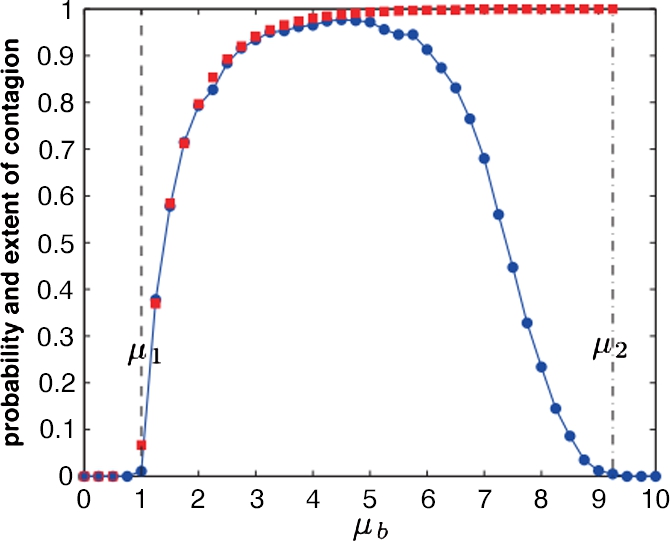
As mentioned above, banks are likely to liquidate a part of their portfolio even before bankruptcy, if an exogenous shock pushes them above their leverage constraint. This is the setting studied in Cont and Schaanning (2017) and Caccioli et al. (2014). In this case, the shocks for which banks start to liquidate as well as the amount liquidated are both smaller than in the setting discussed above. If banks breach their leverage constraint due to an exogenous shock $s_i$ to the value of their illiquid assets, Cont and Schaanning (2017) require that banks liquidate a fraction ${\mathrm{\Gamma }}_i$ of their entire portfolio such that $((1-{\mathrm{\Gamma }}_i){\mathbf{S}}_{it}\cdot {\mathbf{p}}_t+{\hat{A}}_{it}^R)/E_{it}=\bar{\lambda }$. The corresponding liquidated monetary amount for a security j is then $Q_{jt}={\sum }_{i\in \mathcal{B}}{\mathrm{\Gamma }}_i{S}_{ijt}{p}_{jt}$. Again, the sale of the securities is assumed to have market impact such that $p_{jt+1}=p_{jt}(1+f_j(Q_{jt}))$. In contrast to Caccioli et al. (2014), the authors assume that the market impact function $f_j(x)$ is linear in x, where x is the total monetary amount sold rather than the number of shares. Similar market impact functions are used by Greenwood et al. (2015) and Duarte and Eisenbach (2015).

The shape and parameterization of the market impact function is crucial for the practical usage of models of overlapping portfolio contagion. There is a large body of market microstructure literature addressing this question. This literature begins with Kyle (1985), who derived a linear impact function under strong assumptions. More recent theoretical and empirical work indicates that under normal circumstances market impact is better approximated by a square root function (Bouchaud et al., 2008).²⁷

The use of the term “fire sales” in this literature is confusing. Overlapping portfolio contagion can occur even if markets are functioning normally. A good example was the quant meltdown in August 2007. There are also likely to be circumstances in which normal market functioning breaks down due to overload of sellers, generating genuine fire sales; in this circumstance one expects market impact to behave anomalously and the square root approximation to be violated. There is little empirical evidence for this – genuine fire sales most likely occur only for extreme situations such as the crash of 1987 or the flash crash. In common usage the term “fire sale” often refers to any situation where selling of an asset depresses prices, even when the market is orderly.

Cont and Schaanning (2017) calibrate their model to realistic portfolio holdings and market impact parameters and obtain quantitative estimates of the extent of losses due to overlapping portfolio contagion. This provides a good starting point for more sophisticated financial system stress tests that will be discussed in the following sections. The models outlined above can be improved in many ways. Cont and Wagalath (2016) study the effect of overlapping portfolios and fire sales on the correlations of securities in a continuous time setting, where securities prices follow a stochastic process rather than being assumed fixed up to the price impact from fire sales.

5.4 Funding Liquidity Contagion

Funding liquidity contagion has been much less studied than overlapping portfolio or counterparty loss contagion. In the following we will briefly outline some of the considerations that should enter a model of funding liquidity contagion.

In modeling funding liquidity contagion, it is useful to partition an investor's funding into long term funding as well as short term secured and unsecured funding. Only short term funding should be susceptible to funding liquidity contagion as long term funding cannot be withdrawn on the relevant time scales. The availability of secured and unsecured short term funding may be restricted via two channels: a deleveraging channel and a default anticipation channel. The deleveraging channel applies equally to secured and unsecured funding: when a lender needs to deleverage, she can refuse to roll over short term loans, which may in turn force the borrower to deleverage, resulting in a cascade. This channel can be modeled using the same tools applied to overlapping portfolio and counterparty loss contagion. A paper that studies this channel is Gai et al. (2011). The default anticipation channel is different for secured and unsecured funding. In the case of secured funding, a lender might withdraw funding if the quality of the collateral decreases so that the original loan amount is no longer adequately collateralized. In the case of unsecured funding, a lender that questions the credit quality of one its borrowers might anticipate the withdrawal of funding of other lenders to that borrower and therefore withdraw her funding. This mechanism is similar to a bank run and therefore should be modeled as a coordination game, see Diamond and Dybvig (1983) and Morris and Shin (2001). This poses a challenge for heterogeneous agent models and might explain the relative scarcity of the literature on this topic. One notable exception that tries to combine both mechanisms is Anand et al. (2015).

5.5 Interaction of Contagion Channels

So far we have focused on counterparty loss and overlapping portfolio contagion in isolation. Of course, focusing on one channel in isolation only provides a partial view of the system and thus ignores important interaction effects. Indeed, it has been shown by a number of authors that the interaction of contagion channels can substantially amplify the effect of each individual channel (e.g. Poledna et al., 2015; Caccioli et al., 2015; Kok and Montagna, 2013; Arinaminpathy et al., 2012). Although constructing models with multiple contagion channels is difficult, some progress has been made.

Cifuentes et al. (2005) and Caccioli et al. (2015) study the interaction of counterparty loss and overlapping portfolio contagion by combining variants of the contagion processes outlined above into a comprehensive simulation model. In particular, using data from the Austrian interbank system, Caccioli et al. (2015) show that the expected size of a default cascade, conditional on a cascade occurring, can increase by orders of magnitude if overlapping portfolio contagion occurs alongside counterparty loss contagion, rather than in isolation.

In an equilibrium model Brunnermeier and Pedersen (2009) show that market liquidity and funding liquidity can be tightly linked. In particular, consider a market in which intermediaries trade a risky asset and use it as collateral for their secured short term funding. A decline in the price of the risky asset can lead to an increase in the haircut applied on the collateral. An increase in the haircut can be interpreted as a decrease in funding liquidity and can force intermediaries to sell some of their assets. This in turn can lead to a decrease in market liquidity of the asset. Aymanns et al. (2017) show that a similar link between market and funding liquidity can also result from the local structure of liquidity in over-the-counter markets (OTC). The authors show that, when the markets for secured debt and the associated collateral are both OTC, the withdrawal of an intermediary from the OTC markets can cause a liquidity contagion through the networks formed by the two OTC markets. Similar to Caccioli et al. (2015), the authors show that under certain conditions the interaction of two contagion channels – funding and collateral – can drastically amplify the resulting cascade.

Finally, Kok and Montagna (2013) construct a model that attempts to combine counterparty loss, overlapping portfolio and funding liquidity contagion. Such comprehensive stress testing models are the subject of the remainder of this chapter and will be discussed in detail in the following sections.

6.1 What Are Stress Tests?

The insights from the models discussed so far are increasingly used in the tools designed to assess and monitor financial stability. After the crisis of 2008, maintaining financial stability has become a core objective of most central banks.²⁸ One example of such a tool, which has become increasingly prominent over the past years, has been the stress test.²⁹ Stress tests assess the resilience of (parts of) the financial system to crises (Siddique and Hasan, 2012; Scheule and Roesh, 2008; Quagliariello, 2009; Moretti et al., 2008). The central bank designs a hypothetical but plausible adverse scenario, such as a general economic shock (e.g. a negative shock to house prices or GDP) or a financial shock (e.g. a reduction in market liquidity, increased market volatility, or the collapse of a financial institution). Using simulations, the central bank then evaluates how this shock – in the event this scenario were to take place – would affect the resilience of the institution or financial system it tests. Say, for example, that the central bank submits a bank to a stress test. In this case, it would provide the bankers with a hypothetical adverse scenario, and ask them to determine the effect this scenario would have on the bank's balance sheet. If a bank's capital drops below a given threshold, it must raise additional capital. Stress tests evaluate resilience to shocks and link that evaluation to a specific policy consequence intended to enhance that resilience (e.g. raising capital). The process also provides valuable information to regulators and market participants, and helps both to better identify and evaluate risks in the financial system.

6.2 A Brief History of Stress Tests

Stress tests are a relatively novel part of the regulatory toolkit. The potential utility of stress tests had been extensively discussed in the years preceding the financial crisis, and were already used by the International Monetary Fund to evaluate the robustness of countries' financial systems. Banks already designed and conducted stress tests for internal risk management under the Market Risk Amendment of the Basel I Capital Accord, but it was only during the financial crisis that regulators introduced them on a large scale and took a more proactive role in their design and conduct (Armour et al., 2016).

In February 2009 the U.S. Treasury Department introduced the Supervisory Capital Assessment Program (SCAP). This effort was led by Timothy Geither, at a time when uncertainty about the capitalization of banks was still paramount (Schuermann, 2014; Geithner, 2014). Under the auspices of this program the Federal Reserve Board introduced a stress test and required the 19 largest banks in the U.S. to apply it. The immediate motivation was to determine how much capital a bank would need to ensure its viability even under adverse scenarios, and relatedly, whether capital injections from the U.S. tax payer were needed. A secondary motivation was to reduce uncertainty about the financial health of these banks to calm markets and restore confidence in U.S. financial markets (Anderson, 2016; Tarullo, 2016).

In later years, SCAP was replaced by the Comprehensive Capital Analysis and Review (CCAR) and the Dodd–Frank Act Stress Test (DFAST), which have been run on an annual basis since 2011 and 2013, respectively (FED, 2017b, 2017a). These early stress tests gave investors, regulators and the public at large insight into previously opaque balance sheets of banks. They have been credited with restoring trust in the financial sector and thereby contributing to the return of normalcy in the financial markets (Bernanke, 2013).

Across the Atlantic European authorities followed suit and introduced a stress test of their own (EBA, 2017a). This resulted in the first EU stress tests in 2009, overseen by the Committee of European Banking Supervisors (CEBS) (Acharya et al., 2014). Due to concerns about their credibility, the CEBS stress test was replaced in 2011 by stress tests conducted by the European Banking Authority (EBA) (see Ong and Pazarbasioglu, 2014). These have been maintained ever since (EBA, 2017b).

In 2014 the Bank of England also introduced stress tests in line with the American example (BoE, 2014). Around that time, stress tests became a widely used regulatory tool in other countries too (Boss et al., 2007). Now stress tests are regarded as a cornerstone of the post-crisis regulatory and supervisory regime. Daniel Tarullo, who served on the board of the U.S. Federal Reserve from 2009 to 2017 and was responsible for the implementation of stress tests in the U.S., has hailed stress tests as ‘the single most important advance in prudential regulation since the crisis’ (Tarullo, 2014).

Stress tests are not a uniform tool. They can take a variety of forms, which can be helpfully classified along two dimensions. The first dimension concerns their object, or the types of agent that the stress test covers; does the stress test only cover banks, or non-banks as well? In the early days of stress testing, only banks were considered, but now there is an increasing trend toward including non-banks. Given the composition of the financial system in most advanced economies, and the importance of non-banks in these financial systems, it is increasingly acknowledged that excluding non-banks from stress tests would leave regulators with a partial picture of financial stability risks in their jurisdiction. In the United Kingdom, for example, almost half of the assets in the financial system are held by non-banks (Burrows et al., 2015), as is illustrated by a stylized map of the UK financial system depicted in Fig. 7.

The second dimension concerns the scope of the stress test. Generally speaking, stress tests can be used to evaluate the resilience of individual institutions (microprudential stress tests), but could also assess the resilience of a larger group of financial institutions or even of the financial system as a whole (macroprudential stress tests) (Cetina et al., 2015; Bookstaber et al., 2014a). Methodologically speaking, the key difference is that macroprudential stress tests take the feedback loops and interactions between (heterogeneous) financial institutions – as described in Section 4 and Section 5 of this chapter – into account, whereas the microprudential stress tests do not.

Perhaps more than any other financial stability tool, stress tests rely explicitly on the models introduced so far. The following sections will cover micro- and macroprudential stress tests in depth. In each instance, we will first review some representative stress tests and subsequently conclude with an evaluation of their strengths and weaknesses.

7.1 Microprudential Stress Tests of Banks

As noted, microprudential stress tests evaluate the resilience of an individual institution, in this case a bank. Regulators subject the bank to an adverse scenario and evaluate whether a bank has sufficiently high capital buffers³⁰ (and, in some cases, liquid assets³¹) to withstand it.³² If this is not the case, regulators can require the bank to raise additional capital (or liquidity) to enhance its buffers. The idea is that this will make the bank more resilient, and by implication increase the resilience of the financial system as a whole.

Given this general approach, microprudential stress tests for banks tend to follow three steps. First, the regulator designs the adverse scenario the bank is subjected to. As noted, this scenario usually involves an economic and/or financial shock. In some cases, the scenario consists of multiple (exogenous) shocks operating at the same time, sometimes with specified ripple effects affecting other variables, which together create a ‘crisis narrative’ for the bank. The hypothetical scenario a bank is subjected to must be adverse, plausible and coherent. That is, it cannot consist of a set of shocks that, taken together, violate the relationships among variables historically observed or deemed conceivable. Typically, the exogenous shocks affect a set of macro-variables (such as equity prices, house prices, unemployment rate or GDP) as well as financial variables (such as interest rates and credit spreads).

Second, the effect of this scenario on the bank's balance sheet is determined. This determination primarily relates to the effect of the scenario on the bank's capital (and liquidity) buffer, usually expressed as a ratio of capital (liquidity) buffers to assets,³³ and profits. This calculation is based on an evaluation of how the shocks change the values of the assets and liabilities on the bank's balance sheet, as well as on the bank's expected income. Value changes on the balance sheet materialize either through a re-evaluation of the market value (if the asset or liability is marked-to-market), or through a credit shock re-evaluation. These effects are captured by market risk models and credit risk models (such as those described in Siddique and Hasan, 2012; Scheule and Roesh, 2008; Quagliariello, 2009; Moretti et al., 2008). Credit losses for specific assets or asset classes are commonly computed by multiplying the probability of default (PD), the exposure at default (EaD), and the loss given default (LGD). Estimating these variables is therefore key to the credit risk component of stress testing (Foglia, 2009). Value changes to the expected income stream result largely from shocks that affect income on particular assets or asset classes, such as interest rate shocks. This determination matters in the context of the stress test because such income can, in the form of retained earnings, feedback into capital buffers.³⁴ Usually, these microprudential stress test models therefore equate the post-stress regulatory capital buffer to the sum of post-stress retained earning plus regulatory capital³⁵ over the post-stress (risk-weighted³⁶) assets.

Third, once the bank's post-stress capital buffer has been determined, regulators compare it to a hurdle rate. This hurdle rate is usually set at such a level that, when passing it, the bank would withstand the hypothetical scenario without being at risk of bankruptcy. Consequently, if the bank does not meet this hurdle rate, it fails the stress test and is said to be ‘undercapitalized’ (that is, its capital buffer is insufficient). When that happens, the regulator commonly has the authority to require the bank to raise extra capital to increase its buffer, so as to leave it better prepared for adverse scenarios. Microprudential stress tests are thus used as a tool to recapitalize undercapitalized banks, thereby reducing their leverage and increasing their resilience.

7.2 Microprudential Stress Test of Non-Banks

Given the importance of non-bank financial institutions to the financial system,³⁷ it was only a matter of time before the scope of microprudential stress tests would be extended beyond banks. The rationale for doing so is similar to the one that applies to banks: regulators want to understand the resilience of non-bank financial institutions, and where they find fragility they want to be able to amend it. So far, at least three types of non-bank financial institutions are subjected to stress tests: insurers, pension funds and central clearing parties (CCPs).

Like the microprudential stress tests for banks, those for non-bank financial institutions are primarily used to assess capital adequacy in times of distress. However, the methodology used in that assessment differs between the various institutional types, because each type faces a different set (and type) of risks. For example, the balance sheet composition differs for each institution, which in turn means each institution is exposed to different tail risks which should be reflected in the scenario design used in the stress test. Moreover, because of the differences in balance sheet composition, losses materialize in different ways and should be determined using methodologies suitable to each institutional type. Finally, the benchmark each type of institution has to meet in order to ‘pass’ the stress test differs too, because the regulatory requirements vary among different institutional types.³⁸

In sum, the heterogeneity of non-bank financial institutions requires bespoke microprudential stress tests. They all, however, follow the same pattern: they start by setting a hypothetical adverse scenario, evaluate the effect of that scenario on the institution's balance sheet, and compare the post-stress balance sheet to regulatory requirements (hurdles). Table 1 sets out some of the most salient differences between microprudential stress tests for various types of institutions. In what follows, we provide a high-level overview of regulatory stress tests for insurers, pension funds, and central clearing parties.

Insurers and Pension Funds: Insurance stress tests are becoming increasingly common, and have been conducted by the Bank of England (BoE, 2015), the IMF (under its FSAP Program) (Jobst and Andreas, 2014), the U.S. Federal Reserve (Accenture, 2015; Robb, 2015), and the European Insurance and Occupational Pensions Authority (EIOPA) (EIOPA, 2016). Similarly, pension fund stress tests have been conducted by the International Organisation of Pension Fund Supervisors (IOPFS) (Ionescu and Yermon, 2014) and, in the EU, by EIOPA (EIOPA, 2017).

EIOPA's 2016 stress test of life insurers tested each insurer's capital and liquidity adequacy¹ (EIOPA, 2016). When evaluating capital adequacy, the benchmark was that an insurer's assets should exceed its liabilities.² Liquidity adequacy was assessed by performing a cash-flow analysis to investigate whether the timing of insurer's incoming cash-flow (from its assets) matched the insurer's expected cash outflow (resulting from its insurance liabilities).

EIOPA's 2015 stress test of occupational pension funds assessed whether pension payment promises³ could be met in the face of adverse market conditions. The hypothetical adverse scenario was tailored to risks specific to a pension fund. For example, the effect of increased life expectancy (which lengthens the time a pension fund must pay out a pension, and thus increases the cumulative amount of pension payments a pension fund must make) on the pension fund's ability to meet its pension obligations was tested.

Central Clearing Parties: Central clearing parties (CCPs) have been created to mitigate counterparty risk, for example in (simple, or ‘over-the-counter’ (OTC)) derivatives transactions. By doing so, they also reduce the likelihood that counterparty risk causes a cascade of losses, and generates contagion (as has been discussed in Section 5). In this way, well-functioning CCPs can mitigate systemic risk in financial systems.

CCPs operate by stepping in between two contractual counterparties, and becoming, as is commonly noted, ‘the buyer to every seller, and the seller to every buyer’.⁴ Once a contract is ‘cleared’ through a CCP, its counterparties are referred to as ‘clearing members’. As long as no clearing member defaults, the assets and liabilities of the CCP balance out, so that the CCP faces no market risk. That changes when clearing members default, in which case the CCP is exposed to losses. To absorb such losses, the CCP has an elaborate process in place that distributes these losses among all its clearing members as well as its own equity, which is referred to as a ‘default waterfall’ (see Murphy, 2013; Capponi et al., 2017). This default waterfall consists of various contributions of the clearing members (e.g. initial and variation margin, default fund contributions) and some of the CCPs own capital buffer (equity). When losses materialize, these are absorbed by each of the layers in turn, until the CCP's own capital buffer is exhausted and it defaults.⁵

CCPs have become increasingly important after the financial crisis, as regulators require counterparties to frequently-used contracts to clear these contracts through CCPs (ESMA, 2017; Ey, 2013). Individual CCPs have also grown substantially and process very high volumes of trades, leading some to argue that their failure would be catastrophic for the financial system in which they operate (and perhaps beyond) (ESMA, 2015; Murphy, 2013). That is why regulators around the world increasingly carry out microprudential stress tests for CCPs, including the Commodity Futures and Trading Commission (CFTC) in the U.S. (CFTC, 2016), the British and German regulatory authorities (Erbenova, 2015) (this will include a U.S. regulator in 2017) (Robb, 2015), and the European Securities and Markets Authority (ESMA) (ESMA, 2015).

Microprudential stress tests for CCPs focus on whether a CCP's capital buffer (its default waterfall) can absorb losses in a crisis event, to avoid that the CCP defaults. ESMA's CCP stress tests illustrates how such a stress test can be designed (ESMA, 2015).

In ESMA's microprudential CCP stress test from 2015, the adverse scenario included the default of the CCP's two largest clearing members (that is, those two clearing members with the largest contribution to the CCP's default fund),⁶ while the CCP was simultaneously hit by a severe adverse market shift.⁷ Because clearing members often trade in multiple CCPs, the two defaulted clearing members for each CCP were assumed to default in all CCPs where they cleared – which is referred to as cross default contagion.

To assess the extent to which the CCP's capital buffer has been depleted as a consequence of this adverse scenario, the test calculates the losses to each step of the CCP's default waterfall. Losses beyond the absorption capacity of the default waterfall are calculated as well. Taken together, these two criteria are used to judge whether a CCP is sufficiently capitalized.⁸

7.3 Strengths and Weaknesses of Current Microprudential Stress Tests

Microprudential stress tests are valuable from at least three perspectives. First, they give market participants more insight into the opaque balance sheets of the financial institutions being evaluated (Bookstaber et al., 2014a). Opacity coupled with asymmetric information can, especially in times of financial distress, lead to a loss of confidence (Diamond and Dybvig, 1983; Brunnermeier, 2008). If the type and quality of a financial institution's assets and liabilities are unclear, outsiders may conceivably fear the worst and, for example, pull back their funding.⁹ Such responses feed speculative runs which can turn into self-fulfilling prophecies and, ultimately, (further) destabilize the financial system at the worst possible time (He and Xiong, 2012; Diamond and Dybvig, 1983; Martin et al., 2014; Copeland et al., 2014). Credibly executed microprudential stress tests provide insight into an institution's balance sheet, can signal confidence about the institution's ability to withstand severe stress, and create a separating equilibrium that allows solid banks to avoid runs (Ong and Pazarbasioglu, 2014; Bernanke, 2013).¹⁰

Second, microprudential stress tests help financial institutions to improve their own risk-management. By forcing them to assess their resilience to a variety of novel scenarios, stress tests require banks to take a holistic look at their own risk-management practices (Bookstaber et al., 2014a). As a consequence, more banks are now also engaged in serious internal stress tests (Wackerbeck et al., 2016).

Third, microprudential stress tests have proven to be an effective mechanism to recapitalize banks (Armour et al., 2016). In the EU, the stress tests have forced banks to raise their capital by 260 billion euros from 2011 to 2016 (Arnold and Jenkins, 2016), and in the US the risk-weighted regulatory ratio of the banks that took part in the stress test went up from 5.6 percent at the end of 2008 to 11.3 at the end of 2012 (Bernanke, 2013). Against a backdrop of frequent questions about the adequacy of banks' capital buffers,¹¹ in part due to the gaming of risk weights (Behn et al., 2016; Fender and Lewrick, 2015; Groendahl, 2015), many regulators have welcomed the role that stress tests have played to enhance the resilience of banks. Even if microprudential stress tests are not, strictly speaking, designed to assess and evaluate systemic risk, their role in raising capital adequacy standards can have the effect of enhancing resilience (Greenwood et al., 2015).

Despite their strengths in specific areas, the current microprudential stress tests have been criticized on at least four grounds. First, and most importantly from the perspective of this chapter, microprudential stress tests ignore the fact that economies are complex systems (as noted in Section 1) and therefore are ill-suited to capture systemic risk. As discussed in Sections 4 and 5 of this chapter, systemic risk materializes due to interconnections between heterogeneous agents (for example due to overlapping portfolios and funding liquidity contagion). By considering institutions in isolation, microprudential stress tests (largely¹²) ignore the interconnections and interaction between financial institutions that serve to propagate and amplify distress caused by the initial shock resulting from the adverse scenario. Empirical research suggests that this approach substantially underestimates the losses from adverse scenarios (Bookstaber et al., 2014b, also see Section 3). Bernanke (2015), for example, notes that the majority of the losses in the last financial crisis can be traced back to such interactions as opposed to the initial shock emerging from credit losses in subprime mortgage loans.

Second, microprudential stress tests tend to impose an unrealistically large initial shock. Because regulators are aware of the fact that a microprudential modeling strategy does not capture the higher order losses on the balance sheets of individual financial institutions, they use a more severe initial scenario that causes direct losses to compensate for that. To generate a sufficiently large initial shock, the scenario tends to depart quite strongly from reality. Often, the initial scenario posits a substantial increase in the unemployment rate as well as a sharp drop in GDP.¹³ In reality, however, it is uncommon for these conditions to precede a financial crisis, so the stress test might be testing for the wrong type of scenario.¹⁴ Imposing an unrealistic shock – and excluding higher-order effects – can also affect the outcome of the stress test in unexpected ways. In particular, while stress tests with large initial shocks might get the overall losses right, they might fail to accurately capture the distribution of losses across institutions, which ultimately determines which banks survive and which do not. For an investigation of this issue, see for example Cont and Schaanning (2017).

Third, the value of the information produced by microprudential stress tests is increasingly being questioned. The outcomes of stress tests have converged (Glasserman et al., 2015), perhaps because banks seem increasingly able to ‘train to the test’. This has left some to wonder what the information produced by the stress tests is actually worth (Hirtle et al., 2016), and others to conclude that the value of such information has declined over time (Candelon and Sy, 2015). Such concerns have been further fueled by the apparent willingness of some regulators to allow banks to pass the test on the basis of dubious assumptions.¹⁵

Finally, the stress tests are commonly calibrated to the losses incurred during the last financial crisis, raising questions about their relevance in relation to current, let alone future, scenarios – not least because the financial system constantly changes.

8.1 Three Macroprudential Stress Tests

8.1.1 RAMSI Stress Test of the Bank of England

The Bank of England has pioneered the development and use of a macroprudential banking stress test, called the RAMSI model.¹⁸ The model evaluates how adverse shocks transmit through the balance sheets of banks and can cause further contagion effects (Burrows et al., 2012). It is based on earlier research that has been conducted by Bank of England researchers and others (Aikman et al., 2009; Kapadia et al., 2013; Alessandri et al., 2009).

The RAMSI stress test begins as a microprudential stress test. Subsequently, possible feedback effects within the banking system are considered. If the initial shocks have caused a bank to fall below its regulatory capital ratio, or have caused the bank to be shut off of all unsecured funding¹⁹ markets, the bank respectively suffers an insolvency or illiquidity default. Subsequently, the default causes two interbank contagion effects: common asset holding contagion and interbank contagion. The combined effect of the marked-to-market losses and the credit losses can cause other banks to default through insolvency or illiquidity by being shut out of the funding market. If this happens, the loop is repeated. If this does not happen, each bank's net operating expenses are invested in assets such that the bank targets its regulatory risk-weighted target ratio. The credit losses persist, but the marked-to-market losses are assumed to disappear as each asset price returns to its fundamental value. Then, the next time step starts, and the process can be repeated, starting with a balance sheet that includes the credit losses incurred in the previous time step.

Thus, the RAMSI stress test turns a microprudential foundation into a macroprudential model by including interbank contagion effects via common asset holdings, interbank losses and funding liquidity contagion. Fig. 8 summarizes what happens at each step of the RAMSI model.

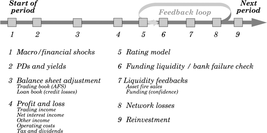
8.1.2 MFRAF Stress Test of the Bank of Canada

Contrary to the RAMSI model, the Bank of Canada's MacroFinancial Risk Assessment Framework (MFRAF) is at its core not a heterogeneous agent model, but a global games model, such as those described in Morris and Shin (2001). In the way it sets up funding runs (i.e. as a global coordination game) it is similar to the seminal model of Diamond and Dybvig (1983) (discussed in Section 5). It captures three sources of risk that banks face (Anand et al., 2014; BoC, 2014, 2012): solvency, liquidity, and spill-over risk (see Fig. 9).

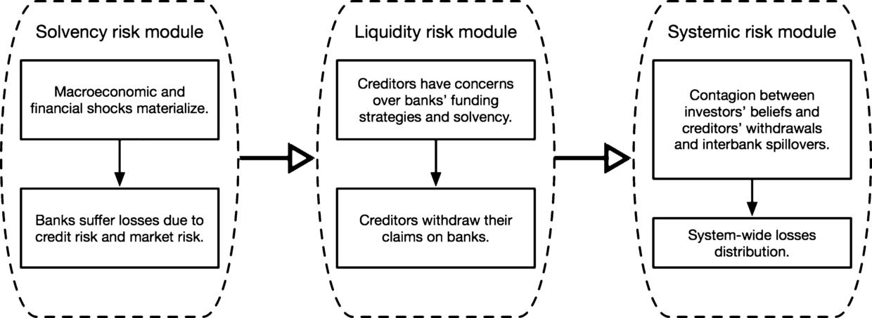
The MFRAF stress test has been applied to the Financial Sector Stability Assessment (FSAP) of the Canadian financial sector conducted by the International Monetary Fund (IMF) in 2014 (IMF, 2014). The 2014 FSAP stress test, which considers the direct effects of adverse shocks on the solvency of banks, is microprudential. When extending it to capture system-wide effects (i.e. liquidity effects and spill-over effects) using MFRAF, overall losses to the capital of the Canadian banks rose with 20 percent. This again shows that microprudential stress tests significantly underestimate system-wide losses. We will now discuss the theoretical underpinnings of the MFRAF stress tests, which builds on research at the Bank of Canada and elsewhere (Anand et al., 2015; Gauthier et al., 2012, 2014).

The theoretical model that underpins the MFRAF stress test is described in Anand et al. (2015) and will be discussed here.²⁰ The model captures how solvency risks, funding liquidity risks, and market risks of banks are intertwined. In essence, this works as follows: a coordination failure between a bank's creditors and adverse selection in the secondary market for the bank's assets interact, leading to a vicious cycle that can drive otherwise solvent banks to illiquidity. Investors' pessimism over the quality of a bank's assets reduces the bank's access to liquidity, which exacerbates the incidence of runs by creditors. This, in turn, makes investors more pessimistic, driving down other banks' access to liquidity. The model does not capture interbank contagion upon default, although this is captured in MFRAF (IMF, 2014).

The key components of the model according to the evolution of the model over time is summarized in Fig. 10.

8.1.3 ABM for Financial Vulnerabilities

The final system-wide stress testing model that will be discussed, the Agent-Based Model (ABM) for Financial Vulnerabilities (Bookstaber et al., 2014b),²¹ captures similar contagion mechanisms as MFRAF, but it does so using a different methodology. The model is designed to investigate the vulnerability of the financial system to asset- and funding-based firesales that can lead to common asset holding contagion.

The financial system is modeled as a combination of banks that act as intermediaries between the cash provider (a representative agent for various types of funds) and the ultimate investors (i.e. the hedge funds). Hedge funds can receive funding from banks for long positions in return for collateral. Banks, in turn, receive funding from the cash provider in return for collateral. Funding and collateral therefore flow in opposite directions, as is illustrated in Fig. 11.

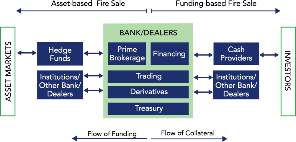
The role of the cash provider c in the model is to provide secured funding to banks.²² Although the cash provider is not actively modeled, it can take two actions. First, it can set the haircut (this can force the hedge fund to engage in fire sales), and second it can pull funding from the banks (this may lead the bank to contribute to pre-default contagion or default).

Hedge funds have a balance sheet that consists of cash and tradable assets on the asset side, and secured loans and equity (and possibly short positions) on the liability side. A hedge fund funds its long positions in assets using funding from banks in the form of repurchase contracts (often referred to as repos).²³ When funding themselves this way, hedge funds receive cash in return for collateral they pledge to the bank. Although the hedge fund does not face a regulatory leverage constraint, it faces an implicit leverage constraint based on the haircut it receives on its collateral. The haircut determines how much equity a hedge fund needs for a given amount of repo funding. If the haircuts on all types of collateral (i.e. on all types of assets that can be pledged as collateral) is the same, and assuming that the bank passes on the haircut it receives from the cash provider, the maximum leverage ${\overline{\lambda }}_{jt}$ of the hedge fund j at time t is given by ${\overline{\lambda }}_{jt}=\frac{1}{h_{cjt}}$. If the leverage of the hedge fund exceeds the maximum leverage,²⁴ the hedge fund is forced to de-lever. It will do so by fire selling assets. This can cause marked-to-market losses for other banks or hedge funds who hold the same assets.

The banks act as an intermediary between buyers and sellers of securities and between lenders and borrowers of funding.²⁵ On the whole, the bank can contribute to financial distress pre-default and post-default in various ways. Pre-default, the bank may have to fire sell assets or to pull funding from the hedge fund (which consequently may also have to engage in firesales) in order to raise cash, de-lever, or pay back funding to the cash provider (if the cash provider pulled its funding). In addition, by passing on an increased haircut to the hedge fund, it can trigger a hedge fund to engage in firesales. Post-default, the bank contributes to exposure losses and further firesale losses.

8.2 Comparing and Evaluating Macroprudential Stress Tests: Five Building Blocks

To comprehensively design, study and evaluate macroprudential stress tests, we introduce a general framework consisting of five building blocks that allow us to break down each stress test in discrete components: (1) types of financial institutions (agents), (2) financial contracts, (3) markets, (4) constraints, and (5) behavior.²⁶ This framework also offers an analytically coherent way to combine the various heterogeneous agent models discussed in Section 4 and Section 5 in order to capture their interactions (see Section 5.5). With such a framework one can capture critical features necessary to be able to capture systemic risk. This section covers these five building blocks and compares the three macroprudential stress tests discussed above²⁷ as we go along (these findings are summarized in Table 2). We will see that these stress tests implement each building block with varying degrees of fidelity to the real world.

8.3 The Calibration Challenge

Calibration is a process to ensure that the estimated parameters of a model match existing data (Turrell, 2016). The design of stress tests can make calibration easier or harder. Calibration is made easier when models are designed so as to either avoid free parameters entirely (by initializing all components to data), or to set up the model so that its parameters can be measured independently on input data rather than based on target data (the data that one wants to fit).⁴² In general, it is therefore useful to design the stress test model so as to closely fit the market infrastructure, because this allows regulators to collect data on each component and then put it together – for example by using the five building blocks used above. A stress test that relies heavily on latent parameters⁴³ will require more assumptions will therefore introduce more uncertainty.

When using the five building blocks (institutions, contracts, markets, constraints and behavior) it becomes clear that the first four can (to a large extent) be data-driven.⁴⁴ Balance sheet data is already collected by regulators, although not always on a contractual level.⁴⁵ This latter step is important, given the importance of contractual constraints in driving specific contagion dynamics (as discussed in Section 8.2). Regulators increasingly recognize this, and have started collecting contract-level data for contractual types considered especially important to financial stability (e.g. Abad et al., 2016).⁴⁶ Because data gaps still persist, the (multi-layered) networks that make up system-wide financial models cannot be completely calibrated to data. In such cases, network reconstruction techniques can generate ‘realistic’ networks based on the known information (e.g. Anand et al., 2018).

Markets are complicated, because the market mechanism has to be modeled correctly. So far, most stress tests abstract away from market infrastructure and instead rely on price impact functions to move prices. The problem is that these functions are driven by ‘market depth’, which is a latent variable and can only be approximated with data about the daily volume of trades and the volatility in the asset class (e.g. Cont and Schaanning, 2017).

The most relevant constraints that drive dynamics, regulatory and contractual constraints could in principle be calibrated to data,⁴⁷ but market constraints have to be inferred and can easily change over time. Internal risk limits can change too and are often proprietary.⁴⁸

The building block for which calibration is most complicated is the last one, behavior. Although behavioral assumptions can be informed by supervisory data and surveys (Bookstaber, 2017), and perhaps even inferred using machine learning techniques, it is bound to change when a new type of crisis hits.⁴⁹ That is why it is important that even if the first four building blocks are (relatively closely) calibrated, the resulting stress tests are explicitly conditional on the behavioral assumption chosen.⁵⁰ It is then possible to change that assumption and run parameter sweeps to get a sense of the effect size of that behavioral assumption. In other words, stress tests might not predict exactly what will happen in a given scenario, but can explore directionally what might happen under a set of what-if scenarios.⁵¹ This can be useful to (1) assess the level of systemic risk; (2) identify potential vulnerabilities in the system; and (3) evaluate the effectiveness of policies designed to mitigate systemic risk.

Calibrating the three macroprudential stress tests discussed above is challenging. The ABMFV may be the easiest to calibrate,⁵² as it captures a realistic market infrastructure (consisting of the first four building blocks). Only behavioral parameters (related to block five) are uncertain, as is the usual case in a social system. It models realistic behavior, but it does not investigate how different behavioral parameters give different dynamics. The RAMSI model relies heavily on a careful calibration of the initial shock and the effect this has on the balance sheet.⁵³ That emphasis on calibrating the initial shock may distract from the most relevant function of any macroprudential model; its evaluation of a financial system's capacity for shock amplification and endogenous dynamics.⁵⁴ Finally, Anand et al. (2015) is a more traditional model that seems much harder to calibrate to data. Its structure is more rigid, and therefore harder to map onto a given market structure. For example, the model's dynamics revolve around a two-period funding contract (and an abstract asset market), but it is not clear how the model can accommodate the variety of contracts that exist in the financial system. On the other hand, Anand et al. (2015) has been used in a data-driven MFRAF stress test.

8.4 Strengths and Weaknesses of the Current Macroprudential Stress Tests

Macroprudential stress tests are strongly complementary to microprudential stress tests, because they allow regulators to assess the resilience of the financial system as a whole (or a larger subset of it) rather than that of individual financial institutions. The current macroprudential stress tests have three related strengths.

First, they provide insights into the interlinkages between financial institutions, mapping out how financial shocks transmit through individual balance sheets and affect other institutions. The data-driven methodology to establish the model setup (as well as the subsequent calibration) provide a promising avenue for future stress tests, but also for further data-driven research into the structure of the financial system (Aikman et al., 2009).

Second, they capture the interactions between various financial institutions and contagion channels that can drive distress, and therefore capture (some of) the feedback effects that characterize the complex nature of the financial system (see Section 4.1 and Section 5). Especially the ABM for Financial Vulnerabilities makes an important contribution by including heterogeneous financial institutions, which is key to allow for emergent phenomena (Bookstaber, 2017).

Third, in addition to capturing solvency risk, or separately investigating solvency and liquidity risk, the current macroprudential stress tests capture funding liquidity risk and the interactions between solvency and liquidity (the interaction between contagion channels has been discussed in Section 5.5). The RAMSI model, for example, not only considers defaults through insolvency, but also through illiquidity, and takes their interaction into account. In case of the MFRAF, a particular strength is that market risk and funding liquidity are endogenously determined. Market risk is based on the degree of adverse selection. Because of asymmetric information, investors offer banks a pooling price for their assets. The pooling price (and hence the market liquidity) lowers if investors become more pessimistic and the quality of the assets is lower. Funding liquidity risk is determined as a function of the bank's credit and market losses (based on general market confidence, and thus as a function of information contagion), its funding composition and maturity profile, and concerns that creditors may have over its future solvency.

Despite these strengths, there is substantial scope for improvement. First, most macroprudential stress tests only cover banks and their creditors, and therefore fail to capture interactions with non-banks that make up a substantial part of the financial system. Non-banks have played an important role in amplifying distress to the banking sector during the 2007–2009 financial crisis (Bernanke, 2015). Therefore, failing to capture non-banks does not just exclude many institutions from the analysis, but also leaves regulators less well-equipped to understand the resilience of the subset of financial institutions they do study. The ABM for Financial Vulnerabilities is an exception, since it does include multiple types of financial institutions, but contrary to the RAMSI and the MFRAF models it is not used as a regulatory stress test.

Second, and relatedly, most macroprudential stress tests capture only a few types of interconnections, even though it is clear that the multiplicity of channels and interconnections between financial institutions plays a critical role in spreading distress (Brunnermeier, 2008) (see also Section 5.5). Notable examples of such contractual linkages include securitized products and credit default swaps.

Third, most current macroprudential stress tests only capture post-default contagion. However, in financial crises pre-default contagion is rampant, often resulting from actions that are prudent from a firm-specific risk-management perspective, but destabilizing from a system-wide perspective. A bank, for example, might engage in precautionary de-leveraging to avoid insolvency (i.e. breaking a leverage constraint), which can add to further negative price spirals. Not capturing such dynamics implies that the total size of contagion, as well as the timing of contagion, is misunderstood.

These three areas of improvement essentially come down to the same point: the current macroprudential stress tests insufficiently capture the diversity of agents and interactions that make up the financial system, and therefore do not do justice to the complex nature of the financial system (or, for that matter, to the insights of the heterogeneous agent model literature, see Sections 4 and 5). One of the important challenges is to devise a modeling strategy that can capture these various effects, and the ABM for Financial Vulnerabilities offers a promising start; the model could easily be extended to capture more types of financial institutions (e.g. central clearing parties, pension funds), financial contracts (e.g. derivative contracts, securitized products), and constraints that drive behavior under stressed circumstances (Cetina et al., 2015; Farmer et al., 2018).

Finally, macroprudential stress tests must be more data-driven⁵⁵ and more carefully calibrated to be credible. Thus, suitably designed system-wide stress tests are enabled to become more credible as regulators collect better (contract-level) data.