
Agent-Based Models for Market Impact and Volatility
Jean-Philippe Bouchaud Capital Fund Management, Paris, France, [email protected]
Abstract
Financial markets display a host of universal “stylized facts” begging for a scientific explanation: Excess volatility, fat tails, and clustered activity are well known and have been studied for many years. More microstructural stylized facts have recently emerged, for example the long memory of the order flow or the square-root dependence of impact on the volume of metaorders. Agent-based models are attempts to account for these stylized facts in a unified manner. Devising faithful microstructural ABMs would allow one to answer crucial questions, such as those related to market stability. Can large orders destabilize markets? Is HFT activity detrimental? Can destabilizing feedback loops be mitigated by adequate regulation? The present review paper summarizes recent work in that direction. We discuss in particular the Santa-Fe zero-intelligence model, which provides a very interesting benchmark, but suffers from important drawbacks as well, such as strong mean-reversion effects. One can enrich the Santa-Fe model as to reproduce both diffusive prices, and the square-root impact law. The underlying mechanism can be well understood in terms of a generic “reaction–diffusion” model for the dynamics of the liquidity, which can be solved analytically. Finally, we argue that the role of “information” is probably overstated in classical theories, while a picture based on a self-reflexive price-impacting order flow has many merits. The recent accumulation of microstructural stylized facts, allowing one to focus on the price formation mechanism, all but confirm that fundamental information plays a relatively minor role in the dynamics of financial markets, at least on short to medium time scales.
Keywords
Microstructure; Order flow; Impact; Agent-based models; Market stability
1 Introduction
Understanding why and how prices move is arguably one of the most important problems in financial economics. The “why” question is intimately related to the information content of prices and the efficiency of markets, and the “how” question is related to the issue of price impact, that has become one of the main theme of research in the recent years, both in academic circles and in trading houses. From a theoretical standpoint, price impact is the transmission belt that allows private information to be reflected by prices. But by the same token, it is also the very mechanism by which prices can be distorted, or even crash, under the influence of uninformed trades and/or fire-sale deleveraging. Price impact is also a cost for trading firms – in fact the dominant one when assets under management become substantial.
Now, the simplest guess is that price impact should be linear, i.e. proportional to the (signed) volume of a transaction. This is in fact the central result of the seminal microstructure model proposed by Kyle in 1985 (Kyle, 1985). This paper has had a profound influence on the field, with over 9500 citations as of November 2017. A linear impact model is at the core of many different studies, concerning for example optimal execution strategies, liquidity estimators, agent-based models, volatility models, etc.
Quite surprisingly, however, the last 20 years have witnessed mounting empirical evidence invalidating classical assumptions. For example, the order flow is found to have long-range autocorrelations, in apparent contradiction with the (nearly) unpredictable nature of price changes. How can this be if order flow impact prices? More strikingly still, empirical results suggest a square-root like growth of impact with traded volume Q, often dubbed the “square-root impact law”, see Section 3.2 below for precise statements and references. This finding is in our opinion truly remarkable, on several counts. First, it is to a large extent universal, across time, markets (including the options markets or the Bitcoin), and execution strategies, suggesting to call it a “law” akin to physical laws. Second, a square-root dependence entails that the last Q/2![]() trades have an impact that is only ∼40% of the first Q/2
trades have an impact that is only ∼40% of the first Q/2![]() . The only possibility for such a strange behavior to hold is that there must exist some memory in the market that extends over a time scale longer than the typical time needed to complete an order (see below for more on this). The second ingredient needed to explain the concavity of the square-root impact is that the last Q/2
. The only possibility for such a strange behavior to hold is that there must exist some memory in the market that extends over a time scale longer than the typical time needed to complete an order (see below for more on this). The second ingredient needed to explain the concavity of the square-root impact is that the last Q/2![]() must experience more resistance than the first Q/2
must experience more resistance than the first Q/2![]() . In other words, after having executed the first half of the order, the liquidity opposing further moves must somehow increase. Still, it is quite a quandary to understand how such non-linear effects can appear, even when the bias in the order flow is very small.
. In other words, after having executed the first half of the order, the liquidity opposing further moves must somehow increase. Still, it is quite a quandary to understand how such non-linear effects can appear, even when the bias in the order flow is very small.
In several recent publications, simple Agent-Based Models (ABM) have been proposed to rationalize the universal square-root dependence of the impact. The argument relies on the existence of slow “latent” order book, i.e. orders to buy/sell that are not necessarily placed in the visible order book but that only reveal themselves as the transaction price moves closer to their limit price. Using both analytical arguments and numerical simulations of an artificial market, one finds that the liquidity profile is V-shaped, with a minimum around the current price and a linear growth of the latent volume as one moves away from that price. This explains why the resistance to further moves increases with the executed volume, and provides a simple explanation – borne out by numerical simulations – for the square-root impact. By the same token, a vanishing expected volume available around the mid-price leads to very small trades having anomalously large impact, as indeed reflected by the singular behavior of the square-root function near the origin.
The aim of the present chapter is to review the recent progress in Agent-Based Microstructure models that attempt to account for the various emergent “stylized facts” of financial markets, in particular the square-root impact just described. We show in particular that zero-intelligence models of order flow fail in general at reproducing the most basic property of prices, namely a random walk like behavior. Interestingly, models must be poised at a “critical point” separating a super-diffusive (trending) market and a sub-diffusive (mean-reverting) market, in such a way that the long range correlation of order flow is precisely balanced by the inertia of the (latent) order book. While all the necessary ingredients seem to be present to understand how fat-tailed distributions and clustered activity effects may emerge within such artificial markets, the final steps needed to complete this program are still not convincingly established, and is an important research objective for the future.
While the literature on ABM for financial markets is extremely abundant (see LeBaron, 2000; Chiarella et al., 2009b; Cristelli et al., 2011 for recent reviews), such models often start from the “mesoscale” (say minutes to days). Agent-Based Models at “microscale” (trades and quotes) have however been considered as well, see Sections 4, 5 and, among others, Bak et al. (1997), Chiarella and Iori (2002), Challet and Stinchcombe (2003), Chiarella et al. (2009a), Preis et al. (2006).
2 The Statistics of Price Changes: A Short Overview
2.1 Bachelier's First Law
The simplest property of financial prices, dating back to Bachelier's thesis (Bachelier, 1900), states that typical price variations grow like the square root of time. More formally, under the assumption that price changes have zero mean (which is a good approximation on short time scales), then the price variogram
(1) V(τ):=E[(pt+τ−pt)2]
grows linearly with time lag τ, such that V(τ)=Dτ![]() .
.
Subsequent to Bachelier's time, many empirical studies noted that the typical size of a given stock's price change tends to be proportional to the stock's price itself. This suggests that price changes should be regarded as multiplicative rather than additive, which, in turn, suggests the use of geometric Brownian motion for price-series modeling. However, over short time horizons – say intraday – there is empirical evidence that price changes are closer to being additive than multiplicative, so we will assume throughout this chapter an additive model of price changes. Still, given the prevalence of multiplicative models for price changes on longer time scales, it has become customary to define the volatility σ in relative terms (even for short timescales), according to the equation
(2) D=σ2p20,
where p0![]() is either the current price or some medium-term average.
is either the current price or some medium-term average.
2.2 Signature Plots
Assume now that a price series is described by
(3) pt=p0[1+t∑t′=1rt′],

where the return series rt![]() is covariance-stationary with zero mean and covariance
is covariance-stationary with zero mean and covariance
(4) Cov(rt′,rt″)=σ20Cr(|t′−t″|).
The case of a random walk with uncorrelated price returns corresponds to Cr(u)=δu,0![]() , where δu,0
, where δu,0![]() is the Kronecker delta function. A trending random walk has Cr(u)>0
is the Kronecker delta function. A trending random walk has Cr(u)>0![]() and a mean-reverting random walk has Cr(u)<0
and a mean-reverting random walk has Cr(u)<0![]() . How does this affect Bachelier's first law?
. How does this affect Bachelier's first law?
One important implication is that the volatility observed by sampling price series on a given time scale τ is itself dependent on that time scale. More precisely, the volatility at scale τ is given by
(5) σ2(τ):=V(τ)p20τ=σ20[1+2τ∑u=1(1−uτ)Cr(u)].

A plot of σ(τ)![]() versus τ is called a volatility signature plot. The case of an uncorrelated random walk leads to a flat signature plot. Positive correlations (which correspond to trends) lead to an increase in σ(τ)
versus τ is called a volatility signature plot. The case of an uncorrelated random walk leads to a flat signature plot. Positive correlations (which correspond to trends) lead to an increase in σ(τ)![]() with increasing τ. Negative correlations (which correspond to mean reversion) lead to a decrease in σ(τ)
with increasing τ. Negative correlations (which correspond to mean reversion) lead to a decrease in σ(τ)![]() with increasing τ.
with increasing τ.
2.3 High-Frequency Noise
Another interesting case occurs when the price pt![]() is soiled by some high-frequency noise, coming e.g. from price discretization effects or from pricing errors. Consider the case where rather than being given by Eq. (3), pt
is soiled by some high-frequency noise, coming e.g. from price discretization effects or from pricing errors. Consider the case where rather than being given by Eq. (3), pt![]() is instead assumed to be governed by
is instead assumed to be governed by
(6) pt=p0[1+t∑t′=1rt′]+ηt,

where ηt![]() is a mean zero, variance σ2η
is a mean zero, variance σ2η![]() noise, uncorrelated with rt
noise, uncorrelated with rt![]() , but is autocorrelated as
, but is autocorrelated as
(7) Cη(τ)=e−τ/τη,
where τη![]() is a short time scale time over which the high-frequency noise is correlated. Eq. (6) is standard in the microstructure (Hasbrouck, 2007), where the observed price is decomposed into a “fundamental” price plus microstructural noise.
is a short time scale time over which the high-frequency noise is correlated. Eq. (6) is standard in the microstructure (Hasbrouck, 2007), where the observed price is decomposed into a “fundamental” price plus microstructural noise.
How does this noise affect the observed volatility? By replacing Cr(τ)![]() in Eq. (5) with Cη(τ)
in Eq. (5) with Cη(τ)![]() , we see that compared to the volatility observed in a price series without noise, the addition of the ηt
, we see that compared to the volatility observed in a price series without noise, the addition of the ηt![]() term in Eq. (6) serves to increase the lag-τ volatility by 2σ2η(1−e−τ/τη)/τ
term in Eq. (6) serves to increase the lag-τ volatility by 2σ2η(1−e−τ/τη)/τ![]() . This additional noise term decays from 2σ2η/τη
. This additional noise term decays from 2σ2η/τη![]() for τ→0
for τ→0![]() , to 0 for τ→∞
, to 0 for τ→∞![]() . The effect of this high-frequency noise on a volatility signature plot is thus akin to mean-reversion, in the sense that it creates a higher short-term volatility than long-term volatility. Note that small pricing errors of ση=0.01%
. The effect of this high-frequency noise on a volatility signature plot is thus akin to mean-reversion, in the sense that it creates a higher short-term volatility than long-term volatility. Note that small pricing errors of ση=0.01%![]() with a one minute life-time would contribute to a very significant excess short-term volatility of 0.3% (daily), to be compared with a typical volatility of 1% for stock indexes.
with a one minute life-time would contribute to a very significant excess short-term volatility of 0.3% (daily), to be compared with a typical volatility of 1% for stock indexes.
2.4 Volatility Signature Plots for Real Price Series
Quite remarkably, the volatility signature plots of most liquid assets (stocks, futures, FX, ...) are nowadays almost flat for values of τ ranging from a few seconds to a few months (beyond which it becomes dubious whether the statistical assumption of stationarity still holds). For example, for the S&P500 E-mini futures contract, which is one of the most liquid contracts in the world, σ(τ)![]() only decreases by about 20% from short time scales (seconds) to long time scales (weeks) – see Fig. 1. The exact form of a volatility signature plot depends on the microstructural details of the underlying asset, but most liquid contracts in this market have a similar volatility signature plot.
only decreases by about 20% from short time scales (seconds) to long time scales (weeks) – see Fig. 1. The exact form of a volatility signature plot depends on the microstructural details of the underlying asset, but most liquid contracts in this market have a similar volatility signature plot.
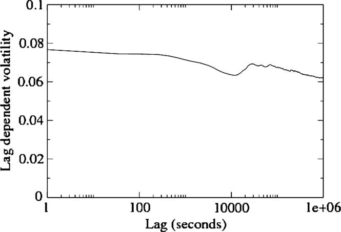
The important conclusion from this empirical result is that long-term volatility is almost entirely determined by the short-term price formation process. Depending on how one views this result, it is either trivial (a simple random walk has this property) or extremely non-intuitive. In fact, one should expect a rather large fundamental uncertainty about the price of an asset, which would translate into substantially larger high-frequency volatility. Although empirical data shows that high-frequency volatility is larger than low-frequency volatility, the size of this effect is small (∼20%![]() ). In a nutshell, long-term volatility seems is closely related to short-term volatility, itself determined by the high-frequency mechanisms of price formation.
). In a nutshell, long-term volatility seems is closely related to short-term volatility, itself determined by the high-frequency mechanisms of price formation.
2.5 Heavy Tails
An overwhelming body of empirical evidence from a vast array of financial instruments (including stocks, currencies, interest rates, commodities, and even implied volatility) show that unconditional distribution of returns has fat tails, which decay as a power law for large arguments and are much heavier than the corresponding tails of the Gaussian distribution, see e.g. Plerou et al. (1999), Gopikrishnan et al. (1999), Gabaix et al. (2006), Cont (2001), Bouchaud and Potters (2003).
On short time scales (between about a minute and a few hours), the empirical density function of returns r can be fit reasonably well by a Student's t distribution, with a distribution f(r)![]() decaying for large r as |r|−1−μ
decaying for large r as |r|−1−μ![]() , is the tail exponent. Empirically, the tail parameter μ is consistently found to be around 3 for a wide variety of different markets, which suggests some kind of universality in the mechanism leading to extreme returns. This universality hints at the fact that fundamental factors are probably unimportant in determining the amplitude of most large price jumps. Interestingly, many studies indeed suggest that large price moves are often not associated to an identifiable piece of news that would rationally explain wild valuation swings (Cutler et al., 1989; Fair, 2002; Joulin et al., 2008).
, is the tail exponent. Empirically, the tail parameter μ is consistently found to be around 3 for a wide variety of different markets, which suggests some kind of universality in the mechanism leading to extreme returns. This universality hints at the fact that fundamental factors are probably unimportant in determining the amplitude of most large price jumps. Interestingly, many studies indeed suggest that large price moves are often not associated to an identifiable piece of news that would rationally explain wild valuation swings (Cutler et al., 1989; Fair, 2002; Joulin et al., 2008).
2.6 Volatility Clustering
Although considering the unconditional distribution of returns is informative, it is also somewhat misleading. Returns are in fact very far from being IID random variables – although they are indeed nearly uncorrelated, as their flat signature plots demonstrate. Therefore, returns are not simply independent random variables drawn from the Student's t distribution. Such an IID model would predict that upon time aggregation, the distribution of returns would quickly converge to a Gaussian distribution on longer time scales. Empirical data indicates that this is not the case, and that returns remain substantially non-Gaussian on time scales up to weeks or even months (Bouchaud and Potters, 2003).
The dynamics of financial markets is in fact highly intermittent, with periods of intense activity intertwined with periods of relative calm. In intuitive terms, the volatility of financial returns is itself a dynamic variable that changes over time with a broad distribution of characteristic frequencies. In more formal terms, returns can be represented by the product of a time-dependent volatility component σt![]() and a directional component ξt
and a directional component ξt![]() ,
,
(8) rt:=σtξt.
In this representation, ξt![]() are IID (but not necessarily Gaussian) random variables of unit variance and σt
are IID (but not necessarily Gaussian) random variables of unit variance and σt![]() are positive random variables with long memory (Cont, 2001; Bollerslev et al., 1994; Muzy et al., 2000; Calvet and Fisher, 2002; Lux, 2008; Chicheportiche and Bouchaud, 2014).
are positive random variables with long memory (Cont, 2001; Bollerslev et al., 1994; Muzy et al., 2000; Calvet and Fisher, 2002; Lux, 2008; Chicheportiche and Bouchaud, 2014).
It is worth pointing out that volatilities σ and scaled returns ξ are not independent random variables. It is well-documented that positive past returns tend to decrease future volatilities and that negative past returns tend to increase future volatilities (i.e., 〈ξtσt+τ〉<0![]() for τ>0
for τ>0![]() ). This is called the leverage effect (Bouchaud et al., 2001). Importantly, however, past volatilities do not give much information on the sign of future returns (i.e., 〈ξtσt+τ〉≈0
). This is called the leverage effect (Bouchaud et al., 2001). Importantly, however, past volatilities do not give much information on the sign of future returns (i.e., 〈ξtσt+τ〉≈0![]() for τ<0
for τ<0![]() ).
).
2.7 Activity Clustering
In view of the long-range correlations of the volatility discussed in the last section, it is interesting to study the temporal fluctuations of market activity itself. Even a cursory look at the time series of mid-point changes suggests a strong degree of clustering in the activity as well.
A more precise way of characterizing this clustering property is to choose a time t and a small dt![]() , and count the number dNt
, and count the number dNt![]() of price changes that occur during the time interval [t,t+dt]
of price changes that occur during the time interval [t,t+dt]![]() (i.e., count dNt=1
(i.e., count dNt=1![]() if the mid-point changed or dNt=0
if the mid-point changed or dNt=0![]() if it did not). The empirical average of dNt
if it did not). The empirical average of dNt![]() provides a way to define the average market activity ‾λ
provides a way to define the average market activity ‾λ![]() , while the covariance Cov[dNt,dNt+τ]
, while the covariance Cov[dNt,dNt+τ]![]() characterizes the temporal structure of the fluctuations in market activity.
characterizes the temporal structure of the fluctuations in market activity.
An increased activity at time t appears to trigger more activity at time t+τ![]() , much like earthquakes are followed by aftershocks. For example, a large jump is usually followed by an increased frequency of smaller price moves. More generally, some kind of “self-excitation” seem to be present in financial markets. This contagion takes place either in the time direction (some events trigger more events in the future) or across different assets (the activity of one stock spills over to other correlated stocks, or even from one market to another). Hawkes processes are mathematical models that capture (part) of these contagion effects, see Bacry et al. (2015) for a review, and Blanc et al. (2016) for some recent extensions.
, much like earthquakes are followed by aftershocks. For example, a large jump is usually followed by an increased frequency of smaller price moves. More generally, some kind of “self-excitation” seem to be present in financial markets. This contagion takes place either in the time direction (some events trigger more events in the future) or across different assets (the activity of one stock spills over to other correlated stocks, or even from one market to another). Hawkes processes are mathematical models that capture (part) of these contagion effects, see Bacry et al. (2015) for a review, and Blanc et al. (2016) for some recent extensions.
2.8 Long Memory in the Order Flow
Another striking stylized fact of financial markets is the persistence in the sign of the order flow. More formally, let εt![]() denote the sign of the tth market order, with εt=+1
denote the sign of the tth market order, with εt=+1![]() for a buy market order and εt=−1
for a buy market order and εt=−1![]() for a sell market order, where t is discrete and counts the number of market orders. In this event-time framework, one can introduce the sign autocorrelation function
for a sell market order, where t is discrete and counts the number of market orders. In this event-time framework, one can introduce the sign autocorrelation function
(9) C(ℓ):=Cov[εt,εt+ℓ],
The surprising empirical result – that holds for many different asset classes (stocks, FX, futures, ...) – is that C(ℓ)![]() decays extremely slowly with ℓ (see Bouchaud et al., 2004, 2006; Lillo and Farmer, 2004; Bouchaud et al., 2009 for a review). Its long time behavior is well-approximated by a power-law ℓ−γ
decays extremely slowly with ℓ (see Bouchaud et al., 2004, 2006; Lillo and Farmer, 2004; Bouchaud et al., 2009 for a review). Its long time behavior is well-approximated by a power-law ℓ−γ![]() with γ<1
with γ<1![]() , corresponding to a so-called long-memory process (Beran, 1994). Typically, γ≈0.5
, corresponding to a so-called long-memory process (Beran, 1994). Typically, γ≈0.5![]() for stock markets and γ≈0.8
for stock markets and γ≈0.8![]() for futures markets (see for example Bouchaud et al., 2004, 2006, 2009; Lillo and Farmer, 2004; and, for futures markets, Mastromatteo et al., 2014a). The origin of this long-memory has been argued to be chiefly due to order splitting (LeBaron and Yamamoto, 2010; Tóth et al., 2015) rather than direct herding. Importantly, the long memory of order signs and long-memory in activity fluctuations are distinct phenomena, with no logical relation to one another (it is easy to build models that have one type of long memory, but not the other).
for futures markets (see for example Bouchaud et al., 2004, 2006, 2009; Lillo and Farmer, 2004; and, for futures markets, Mastromatteo et al., 2014a). The origin of this long-memory has been argued to be chiefly due to order splitting (LeBaron and Yamamoto, 2010; Tóth et al., 2015) rather than direct herding. Importantly, the long memory of order signs and long-memory in activity fluctuations are distinct phenomena, with no logical relation to one another (it is easy to build models that have one type of long memory, but not the other).
The persistence in the sign of the order flow leads to an apparent “efficiency paradox”, which asks the question of how prices can remain unpredictable when order flow (which impacts the price directly) is so predictable. We will come back on this issue in Section 5.
2.9 Summary
The above short review of the statistical properties of prices has left aside a host of other interesting regularities, in particular concerning inter-asset correlations, long-term behavioral anomalies, trend following effects and other “factor” dynamics, etc. The main message of this section is that price changes are remarkably uncorrelated over a large range of frequencies, with little signs of price adjustments or tâtonnement at high frequencies. The long-term volatility appears to be determined by the short-term, high frequency movements of the price.
In fact, the frequency of news that would affect the fundamental value of financial assets is much lower than the frequency of price changes themselves. As Cutler, Poterba, and Summers state it: The evidence that large market moves often occur on days without any identifiable major news releases, casts doubt on the view that stock price movements are fully explicable by news. It is as if price changes themselves are the main source of news, and feedback as to create self-induced excess volatility and, most probably, price jumps that occur without any news at all. Interestingly, all quantitative volatility/activity feedback models (such as ARCH/GARCH models and the like, or Hawkes processes; see Bollerslev et al., 1994; Chicheportiche and Bouchaud, 2014; Bacry et al., 2015; Hardiman et al., 2013) suggest that at least 80% of the price variance is induced by self-referential effects. This adds credence to the idea that a lion's share of the short to medium term activity of financial markets is unrelated to any fundamental information or economic effects.
From a scientific point of view, this is extremely interesting, since it opens the path to building a theory of price moves that is mostly based on modeling the endogenous, self-exciting dynamics of markets, and not on long-term fundamental effects. One particularly important question is to understand the origin and the mechanisms leading to price jumps, which seem to have a similar structure on all traded, liquid markets (again indicating that fundamental factors are probably unimportant at short time scales).
3 The Square-Root Impact Law
3.1 Introduction
Assume that following a decision to trade (whatever the underlying reason might be) one has to buy (or sell) some quantity Q on the market. Ideally, one would like to execute it immediately, “at the market price”. However, unless the quantity Q is smaller than the available volume at the best quote, this is simply not possible. There is no such thing as a “market price”. The market price is not only different for buy trades and sell trades, it really only makes sense for infinitesimal volumes, when the trade can be executed in one shot, such that impact on later trades can be neglected. For volumes typical of large financial institutions – say 1% of the market capitalization of a given stock – there is just not enough liquidity in the whole Limit Order Book (LOB) to match the required quantity Q.
Large trades should thus be split in small chunks. This incremental execution aims at allowing the latent liquidity to reveal itself and refill the LOB with previously undisclosed orders (what we call later the “latent” order book). This should, in principle, considerably improve the price obtained compared to an immediate execution with market orders that would otherwise penetrate deep into the book and possibly even destabilize the market.
The sequence of trades that comes from a single investment decision is known as a metaorder. How does a metaorder of size Q impact the price? From the point of view of investors: what is the true cost of trading? How does it depend on market conditions, execution strategies, and time horizon, etc.? From the point of view of regulators: can large metaorders destabilize markets? Is marked-to-market accounting wise when, as emphasized above, the market price is at best meaningful for infinitesimal volumes, but not for large investment portfolios that would substantially impact the price upon unwinding?
3.2 Empirical Evidence
Naively, one expects the impact of a metaorder to be linear in its volume Q. It is also what standard theoretical models of impact predict, such as the famous Kyle model (Kyle, 1985). However, there is now overwhelming empirical evidence ruling out the simple linear impact law, and suggesting instead a concave, square-root-like growth of impact with volume, often dubbed the “square-root impact law”. The impact of a metaorder is surprisingly universal: the square-root law has been reported in many different studies, both academic and professional, since the early eighties (Loeb, 1983). It appears to hold for completely different markets (equities, futures, FX, options (Tóth et al., 2016), or even the Bitcoin; Donier and Bonart, 2015), epochs (pre-2005, when liquidity was mostly provided by market makers, and post-2005, with electronic markets dominated by HFT), types of microstructure (small ticks versus large ticks), market participants and underlying trading strategies (fundamental, technical, etc.), and styles of execution (using limit or market orders). In all these cases, the impact of a meta-order of volume Q is well described by (Torre and Ferrari, 1997; Grinold and Kahn, 1999; Almgren et al., 2005; Moro et al., 2009; Tóth et al., 2011; Mastromatteo et al., 2014a; Gomes and Waelbroeck, 2014; Bershova and Rakhlin, 2013; Brokmann et al., 2015)1
(10) I(Q,T)≈YσT(QVT)δ(Q≪VT)

where δ is an exponent in the range 0.4–0.7, Y is a numerical coefficient of order unity (Y≈0.5![]() for US stocks), and σT
for US stocks), and σT![]() and VT
and VT![]() are, respectively, the average contemporaneous volatility on the time horizon T and the average contemporaneous traded volume over time T. Note that Eq. (10) is dimensionally correct (in the sense that the dimension of Q and VT
are, respectively, the average contemporaneous volatility on the time horizon T and the average contemporaneous traded volume over time T. Note that Eq. (10) is dimensionally correct (in the sense that the dimension of Q and VT![]() cancel out, while impact and volatility are indeed expressed as price percentage). Kyle's model instead leads to δ=1
cancel out, while impact and volatility are indeed expressed as price percentage). Kyle's model instead leads to δ=1![]() , with a Kyle “lambda” parameter equal to YσT/VT
, with a Kyle “lambda” parameter equal to YσT/VT![]() .
.
3.3 A Very Surprising Law
This square-root impact law is extremely well established empirically but extremely surprising theoretically. As mentioned in the introduction, one finds that the second half of a metaorder of size impacts the price much less than the first half, in fact, a square-root impact gives √2−1=0.4142...![]() times less. How can this be? Surely if one traded the second half a very long time after the first half, impact should be additive again, as the memory of the first trade would evaporate. This clearly shows that there must be some kind of “memory time” Tm
times less. How can this be? Surely if one traded the second half a very long time after the first half, impact should be additive again, as the memory of the first trade would evaporate. This clearly shows that there must be some kind of “memory time” Tm![]() in financial markets, such that impact is square root for T≪Tm
in financial markets, such that impact is square root for T≪Tm![]() but additivity is recovered for T≫Tm
but additivity is recovered for T≫Tm![]() , when all memory of past trades is lost. We will hypothesize in Sections 5, 6 that this memory is in fact imprinted in the “latent” order book alluded to above, that stores the outstanding liquidity that cannot be executed immediately.
, when all memory of past trades is lost. We will hypothesize in Sections 5, 6 that this memory is in fact imprinted in the “latent” order book alluded to above, that stores the outstanding liquidity that cannot be executed immediately.
Note that the relevant ratio here is the volume of the metaorder Q to the market volume VT![]() over the execution time, and not, as could have been naively anticipated, the ratio of Q over total the market capitalization M
over the execution time, and not, as could have been naively anticipated, the ratio of Q over total the market capitalization M![]() of the asset. That one should trade 1% of the market capitalization M
of the asset. That one should trade 1% of the market capitalization M![]() of a stock to move its price by 1% would look reasonable at first sight. It was in fact common lore in the 80's, when impact was deemed totally irrelevant for quantities representing a few basis points of M
of a stock to move its price by 1% would look reasonable at first sight. It was in fact common lore in the 80's, when impact was deemed totally irrelevant for quantities representing a few basis points of M![]() . But M
. But M![]() is (for stocks) 200 times larger than VT
is (for stocks) 200 times larger than VT![]() itself, so that Q/M≪Q/VT
itself, so that Q/M≪Q/VT![]() . Therefore a Q/M
. Therefore a Q/M![]() scaling would have meant a much smaller impact than the one observed in practice. The non-linear square-root behavior for Q≪VT
scaling would have meant a much smaller impact than the one observed in practice. The non-linear square-root behavior for Q≪VT![]() furthermore substantially amplifies the impact of small metaorders: executing 1% of the daily volume moves the price (on average) by √1%=10%
furthermore substantially amplifies the impact of small metaorders: executing 1% of the daily volume moves the price (on average) by √1%=10%![]() of its daily volatility. The main conclusion here is that impact, even of relatively small metaorders, is a surprisingly large effect.
of its daily volatility. The main conclusion here is that impact, even of relatively small metaorders, is a surprisingly large effect.
Let us highlight another remarkable property of the strict square-root impact, which that I(Q,T)![]() is approximately independent of the execution time horizon T, and only determined by the total exchanged volume Q. This follows from the fact that σT∝√T
is approximately independent of the execution time horizon T, and only determined by the total exchanged volume Q. This follows from the fact that σT∝√T![]() whereas VT∝T
whereas VT∝T![]() , so that the T dependence cancels out in Eq. (10). In economics term, this makes sense: the market price has to adapt to a certain change of global supply/demand εQ, quite independently on how this volume is actually executed. A more detailed, “Walrasian” view of this highly non-trivial statement is provided in Section 6.
, so that the T dependence cancels out in Eq. (10). In economics term, this makes sense: the market price has to adapt to a certain change of global supply/demand εQ, quite independently on how this volume is actually executed. A more detailed, “Walrasian” view of this highly non-trivial statement is provided in Section 6.
Let us note however that the square-root impact law (10) is only approximately valid in a certain domain of parameters, as with any empirical law. For example, as we have mentioned already, the execution time T should not be longer than a certain “memory time” Tm![]() of the market. The second obvious limitation is that the ratio Q/VT
of the market. The second obvious limitation is that the ratio Q/VT![]() should be small, such that the metaorder remains a small fraction of the total volume VT
should be small, such that the metaorder remains a small fraction of the total volume VT![]() and that the impact itself is small compared to the volatility. In the case where Q/VT
and that the impact itself is small compared to the volatility. In the case where Q/VT![]() becomes substantial, one must enter a different regime as the metaorder becomes a large perturbation to the normal course of the market.
becomes substantial, one must enter a different regime as the metaorder becomes a large perturbation to the normal course of the market.
Finally, let us discuss some recurrent misconceptions or confusions that exist in the literature concerning the impact of metaorders:
- • First, we emphasize that the impact of a metaorder of volume Q is not equal to the aggregate impact of order imbalance ΔV=Q
 , which is in fact linear for small ΔV, and not square-root like (Bouchaud et al., 2009; Patzelt and Bouchaud, 2018). One cannot measure the impact of metaorders without being able to identify the origin of the trades, and correctly ascribe them to a given investor executing an order.
 - • The square-root impact law applies to slow metaorders composed of several individual trades, but not to these individual trades themselves. Universality, if it holds, can only result from some “mesoscopic” properties of the supply and demand in financial markets, that are insensitive to the way markets are organized at the microscale. This would explain, for example, why the square-root law holds equally well in the pre-HFT era (say before 2005) and since the explosion of electronic, high frequency market making (after 2005).
- • Conversely, at the single trade level, one expects that microstructure effects (tick size, continuous markets vs. batch auctions, etc.) play a strong role. In particular, the impact of a single market order of size q does not behave like a square-root, although it behaves as a concave function of q (Bouchaud et al., 2009). But this concavity has no immediate relation with the concavity of the impact of metaorders.
3.4 Theoretical Ideas
The square-root law was not anticipated by financial economists: classical models, such as the Kyle model, all suggested or posited a linear behavior. It is an interesting case where empirical data compelled the finance community to accept that reality was fundamentally different from theory. Several stories have been proposed since the mid-nineties to account for the square-root impact law.
The first attempt, due to the Barra group (Torre and Ferrari, 1997) and Grinold and Kahn (1999), argues that the square-root behavior is a consequence of market-markers getting compensated for their inventory risk. Assume that the metaorder of volume Q is absorbed by market-makers who will need to slowly offload their position later on. The amplitude of an adverse move of the price during this unwinding phase is given by ∼σ√Toff.![]() , where Toff.
, where Toff.![]() is the time needed to offload an inventory of size Q. It is reasonable to assume that Toff.
is the time needed to offload an inventory of size Q. It is reasonable to assume that Toff.![]() is proportional to Q and inversely proportional to the trading rate of the market V. If market-makers respond to the metaorder by moving the price in such a way that their profit is of the same order as the risk they take, then indeed I∝σ√Q/V
is proportional to Q and inversely proportional to the trading rate of the market V. If market-makers respond to the metaorder by moving the price in such a way that their profit is of the same order as the risk they take, then indeed I∝σ√Q/V![]() , as found empirically. However, this story assumes no competition between market-makers. Indeed, inventory risk is diversifiable over time and on the long run averages to zero. Charging an impact cost compensating for the inventory risk of each metaorder would lead to formidable profits and necessarily attract competing liquidity providers.
, as found empirically. However, this story assumes no competition between market-makers. Indeed, inventory risk is diversifiable over time and on the long run averages to zero. Charging an impact cost compensating for the inventory risk of each metaorder would lead to formidable profits and necessarily attract competing liquidity providers.
Another story, proposed by Gabaix et al. (2003, 2006), ascribes the square-root impact law to the fact that the optimal execution horizon T⁎![]() for “informed” metaorders of size Q grows like T⁎∼√Q
for “informed” metaorders of size Q grows like T⁎∼√Q![]() . Since during that time the price is expected to move linearly in the direction of the trade as information gets slowly revealed, the apparent peak impact behaves as √Q
. Since during that time the price is expected to move linearly in the direction of the trade as information gets slowly revealed, the apparent peak impact behaves as √Q![]() . However, this scenario would imply that the impact during the metaorder is linear in the executed quantity q, at variance with empirical data: the impact path itself behaves as a square-root of q, at least when the execution schedule is flat.
. However, this scenario would imply that the impact during the metaorder is linear in the executed quantity q, at variance with empirical data: the impact path itself behaves as a square-root of q, at least when the execution schedule is flat.
Recently, Farmer et al. (2013) have proposed yet another theory which is very reminiscent of the Glosten–Milgrom model (Glosten and Milgrom, 1985) that competitively sets the size of the bid–ask spread. One assumes metaorders with a power-law distributed volume Q come one after the other. Market-makers attempt to guess whether the metaorder will continue or stop at the next time step, and set the price such that (a) it is a martingale and (b) the average execution price compensates for the information contained in the metaorder (“fair pricing”). Provided the distribution of metaorder sizes behaves as Q−5/2![]() , these two conditions lead to a square-root impact law. Although enticing, this theory has difficulty explaining why the square-root law holds even when the average impact is smaller than, or of the same order as the bid–ask spread and/or the trading fees – which should in principle strongly affect the market-makers' fair pricing condition. Furthermore, the square-root impact law appears to be much more universal than the distribution of the size of metaorders. In the case of Bitcoin, for example, the square-root law holds very precisely while the distribution of metaorders behaves as Q−2
, these two conditions lead to a square-root impact law. Although enticing, this theory has difficulty explaining why the square-root law holds even when the average impact is smaller than, or of the same order as the bid–ask spread and/or the trading fees – which should in principle strongly affect the market-makers' fair pricing condition. Furthermore, the square-root impact law appears to be much more universal than the distribution of the size of metaorders. In the case of Bitcoin, for example, the square-root law holds very precisely while the distribution of metaorders behaves as Q−2![]() rather than Q−5/2
rather than Q−5/2![]() (Donier and Bonart, 2015).
(Donier and Bonart, 2015).
The universality of the square-root law suggests that its explanation should rely on minimal, robust ingredients that would account for its validity is different markets (from stocks to Bitcoin) and different epochs (from pit markets to electronic platforms). We will present in Sections 5 and 6 a minimal agent-based model of the dynamics of supply and demand. This framework, originally put forth by Tóth et al. (2011) and much developed since, provides a natural interpretation of the square-root law and its apparent universality.
4 The Santa-Fe “Zero-Intelligence” Model
In this section, we introduce a (over-)simplified framework for describing the co-evolution of liquidity and prices, at the level of the Limit Order Book.2 This model was initially proposed and developed by a group of scientists then working at the Santa Fe Institute, see Daniels et al. (2003), Smith et al. (2003), Farmer et al. (2005).3 After describing the Santa-Fe model and the price dynamics it generates, we will discuss some of its limitations. (Note that what we call here the Santa-Fe model is not the stock market agent-based model (Palmer et al., 1994) but rather the more recent particle-based limit order book model.)
4.1 Model Definition
Consider the continuous-time temporal evolution of a set of particles on a one-dimensional lattice of mesh size equal to one tick ϑ. Each location on the lattice corresponds to a specified price level in the LOB. Each particle is either of type A, which corresponds to a sell order, or of type B, which corresponds to a buy order. Each particle corresponds to an order of a fixed size υ0![]() which we can arbitrarily set to unity. Whenever two particles of opposite type occupy the same point on the pricing grid, an annihilation A+B→∅
which we can arbitrarily set to unity. Whenever two particles of opposite type occupy the same point on the pricing grid, an annihilation A+B→∅![]() occurs, to represent the matching of a buy order and a sell order. Particles can also “evaporate”, to represent the cancellation of an order by its owner. The position of the leftmost A particle defines the ask price a(t)
occurs, to represent the matching of a buy order and a sell order. Particles can also “evaporate”, to represent the cancellation of an order by its owner. The position of the leftmost A particle defines the ask price a(t)![]() , and he position of the rightmost B particle defines the bid price b(t)
, and he position of the rightmost B particle defines the bid price b(t)![]() . The mid-price is m(t)=(b(t)+a(t))/2
. The mid-price is m(t)=(b(t)+a(t))/2![]() , and the bid–ask spread s(t)
, and the bid–ask spread s(t)![]() is a(t)−b(t)
is a(t)−b(t)![]() .
.
In the Santa-Fe “Zero-Intelligence” model, order flows are completely random and assumed to be governed by the following stochastic processes,4 where all orders have size υ0=1![]() :
:
- • At each price level p⩽m(t)
 (resp. p⩾m(t)
 ), buy (resp. sell) limit orders arrive as a Poisson process with rate λ, independently of p.
 - • Buy/Sell market orders arrive as Poisson processes, each with rate μ.
- • Each outstanding buy (resp. sell) limit order is canceled according to a Poisson process with rate ν.
- • All event types are mutually independent.
The first two rules mean that the mid-price m(t)![]() is the reference price around which the order flow organizes. Whenever a buy (respectively, sell) market order x arrives at time tx
is the reference price around which the order flow organizes. Whenever a buy (respectively, sell) market order x arrives at time tx![]() , it annihilates a sell limit order at the price a(tx)
, it annihilates a sell limit order at the price a(tx)![]() (respectively, buy limit order at the price b(tx)
(respectively, buy limit order at the price b(tx)![]() ), and thereby causes a transaction. Therefore, the interacting flows of market order arrivals, limit order arrivals, and limit order cancellations together fully specify the temporal evolution of the LOB, and in particular the mid-price m(t)
), and thereby causes a transaction. Therefore, the interacting flows of market order arrivals, limit order arrivals, and limit order cancellations together fully specify the temporal evolution of the LOB, and in particular the mid-price m(t)![]() .
.
4.2 Basic Intuition
Before investigating the model in detail, we first appeal to intuition to discuss some of its more straightforward properties. First, each of the parameters λ, μ, and ν are rate parameters, with units of inverse time. Therefore, any observable related to the equilibrium distribution of volumes, spreads, or gaps between filled prices can only depend on ratios of λ, μ, and ν, to cause the units to cancel out.
Second, the approximate distributions of queue sizes can be derived by considering the interactions of the different types of order flows at different prices. Because market order arrivals only influence activity at the best quotes, it follows that very deep into the LOB, the distribution of queue sizes V reaches a stationary state that is independent of the distance from m(t)![]() , given by
, given by
(11) Pst.(V)=e−V⁎V⁎VV!,V⁎=λν.

Two extreme cases are possible:
- • A sparse LOB, corresponding to V⁎≪υ0=1
 , where most price levels are empty while some are only weakly populated. This case corresponds to very small-tick assets.
 - • A dense LOB, corresponding to V⁎≫υ0=1
 , where all price levels are populated with a large number of orders. This corresponds to large-tick assets, at least close enough to the mid-point so that the assumption that λ is constant is reasonable.
In reality, one observes that λ decreases with increasing distance from m(t)![]() . Therefore, even in the case of large-tick stocks, we expect a cross-over between a densely populated LOB close to the best quotes and a sparse LOB far away from them. This does not, however, imply that there are no buyers or sellers who wish to trade at prices far away from the current mid-point. As we will argue in Sections 5, 6, the potential number of buyers (respectively, sellers) is expected to grow with increasing distance from m(t)
. Therefore, even in the case of large-tick stocks, we expect a cross-over between a densely populated LOB close to the best quotes and a sparse LOB far away from them. This does not, however, imply that there are no buyers or sellers who wish to trade at prices far away from the current mid-point. As we will argue in Sections 5, 6, the potential number of buyers (respectively, sellers) is expected to grow with increasing distance from m(t)![]() , but most of the corresponding liquidity is latent, and only becomes revealed as m(t)
, but most of the corresponding liquidity is latent, and only becomes revealed as m(t)![]() decreases (respectively, increases).
decreases (respectively, increases).
The above distribution of queue sizes is not accurate for prices close to m(t)![]() . If d denotes the distance between a given price and m(t)
. If d denotes the distance between a given price and m(t)![]() , then for smaller values of d, it becomes increasingly likely that a given price was actually the best price in the recent past. Correspondingly, limit orders are depleted not only because of cancellations but also because of market orders that may have hit that queue. Heuristically, one expects that the average size of the queues is given by
, then for smaller values of d, it becomes increasingly likely that a given price was actually the best price in the recent past. Correspondingly, limit orders are depleted not only because of cancellations but also because of market orders that may have hit that queue. Heuristically, one expects that the average size of the queues is given by
V⁎≈λ−μϕeff(d)ν,
where ϕeff(d)![]() is the fraction of time during which the corresponding price level was the best quote in the recent past (of duration ν−1
is the fraction of time during which the corresponding price level was the best quote in the recent past (of duration ν−1![]() , beyond which all memory is lost). This formula says that queues tend to be smaller on average close to the mid-point, simply because the market order flow plays a greater role in removing outstanding limit orders. One therefore expects that the average depth profile is an increasing function of d, at least close to d=0
, beyond which all memory is lost). This formula says that queues tend to be smaller on average close to the mid-point, simply because the market order flow plays a greater role in removing outstanding limit orders. One therefore expects that the average depth profile is an increasing function of d, at least close to d=0![]() where λ can be considered as a constant. This is indeed what is observed in empirical data of LOB volume profiles, see Bouchaud et al. (2002, 2009), where a simple theory describing the shape of an LOB's volume profile is also given.
where λ can be considered as a constant. This is indeed what is observed in empirical data of LOB volume profiles, see Bouchaud et al. (2002, 2009), where a simple theory describing the shape of an LOB's volume profile is also given.
Next, we consider the size of the spread s(t)![]() . For large-tick stocks, the bid and ask queues will both typically be long and s(t)
. For large-tick stocks, the bid and ask queues will both typically be long and s(t)![]() will spend most of the time equal to its smallest possible value of one tick, s(t)=ϑ
will spend most of the time equal to its smallest possible value of one tick, s(t)=ϑ![]() . For small-tick stocks, however, the spread may become larger. In this case, the probability per unit time that a new limit order arrives inside the spread is given by (ˆs−1)λ
. For small-tick stocks, however, the spread may become larger. In this case, the probability per unit time that a new limit order arrives inside the spread is given by (ˆs−1)λ![]() (because both buy and sell limit orders can fall on the ˆs−1
(because both buy and sell limit orders can fall on the ˆs−1![]() available intervals inside the spread s=ˆsϑ
available intervals inside the spread s=ˆsϑ![]() ), and the probability per unit time that an order at the best quotes is removed by cancellation or by an incoming market order is given by 2(μ+ν)
), and the probability per unit time that an order at the best quotes is removed by cancellation or by an incoming market order is given by 2(μ+ν)![]() . The equilibrium spread size is such that these two effects compensate,
. The equilibrium spread size is such that these two effects compensate,
seq.≈ϑ[1+2μ+νλ].

Although hand-waving, this argument gives a good first approximation of the average spread. In particular, the result that a large flux of market orders μ opens up the spread sounds reasonable.
4.3 Simulation Results
Deriving analytical results about the behavior of the Santa Fe model is deceptively difficult (Smith et al., 2003). By contrast, simulating the model is relatively straightforward. The Santa Fe model is extremely rich, so many output observables can be studied in this way. We restrict here to three particularly relevant topics:
- 1. The ratio between the mean first gap behind the best quote (i.e., the price difference between the best and second-best quotes) and the mean spread s;
- 2. The volatility and signature plot of the mid-price;
- 3. The mean impact of a market order and the mean profit of market-making.
Numerical results show that the model does a good job of capturing some of these properties, but a less good job at capturing others, due to the many simplifying assumptions that it makes. For example, when λ,μ,ν![]() are calibrated on real data, the model makes good predictions of the mean bid–ask spread, as first emphasized by Farmer et al. (2005). However, the price series that it generates show significant mean-reverting behavior, except when the memory time Tm=ν−1
are calibrated on real data, the model makes good predictions of the mean bid–ask spread, as first emphasized by Farmer et al. (2005). However, the price series that it generates show significant mean-reverting behavior, except when the memory time Tm=ν−1![]() is very short (Daniels et al., 2003; Smith et al., 2003). As noticed in Section 2.4, such mean-reversion is usually not observed in real markets. Moreover, the model predicts volatility to be too small for large-tick stocks and too large for small-tick stocks, and furthermore creates strong arbitrage opportunities for market-making strategies that do not exist in real markets. These weaknesses of the model provide insight into how it might be improved, by including additional effects such as the long-range correlations of order flow or some simple strategic behaviors from market participants (see Section 5).
is very short (Daniels et al., 2003; Smith et al., 2003). As noticed in Section 2.4, such mean-reversion is usually not observed in real markets. Moreover, the model predicts volatility to be too small for large-tick stocks and too large for small-tick stocks, and furthermore creates strong arbitrage opportunities for market-making strategies that do not exist in real markets. These weaknesses of the model provide insight into how it might be improved, by including additional effects such as the long-range correlations of order flow or some simple strategic behaviors from market participants (see Section 5).
4.3.1 The Gap-to-Spread Ratio
Let us consider the mean gap between the second-best quote and the best quote, compared to the mean spread itself. We call this ratio the gap-to-spread ratio. The gap-to-spread ratio is interesting since it is to a large extent insensitive to the problem of calibrating the parameters correctly (and of reproducing the mean bid–ask spread exactly).
Fig. 2 shows the empirical gap-to-spread ratio versus the gap-to-spread ratio generated by simulating the Santa Fe model, for a selection of 13 US stocks with different tick sizes (Bouchaud et al., 2018). For large-tick stocks, the model predicts that both the spread and the gap between the second-best and best quotes are nearly always locked to 1 tick, so the ratio is itself simply equal to 1. In reality, however, the dynamics is more subtle. The bid–ask spread actually widens more frequently than the Santa Fe model predicts, such that the empirical gap-to-spread ratio is in fact in the range 0.8–0.95. This discrepancy becomes even more pronounced for small-tick stocks, for which the empirical gap-to-spread ratio typically takes values around 0.15–0.2, but for which the Santa Fe model predicts a gap-to-spread ratio as high as 0.4. In other words, when the spread is large, the second best price tends to be much closer to the best quote in reality than it is in the model. As we will see in below this turns out to have an important consequence for the impact of market orders in the model.

This analysis of the gap-to-spread ratio reveals that an important ingredient is missing from the Santa Fe model. When the spread is large, real liquidity providers tend to place new limit orders inside the spread, but still close to the best quotes, and thereby typically only improve the quote price by one tick at a time. This leads to gaps between the best and second-best quotes that are much smaller than those predicted by the assumption of uniform arrivals of limit orders at all prices beyond the mid-price. One could indeed modify the Santa Fe specification to account for this empirically observed phenomenon of smaller gaps for limit orders that arrive inside the spread, but doing so comes at the expense of adding extra parameters, see Mike and Farmer (2008).
4.3.2 The Signature Plot
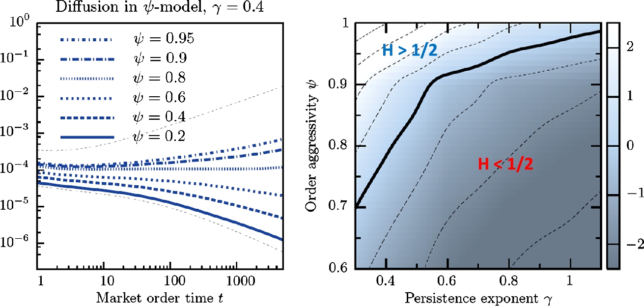
When simulating the Santa Fe model, the lag-dependent volatility σ(τ)![]() of the mid-price, and the corresponding signature plot (see Section 2.4), both reveal that the model exhibits some excess volatility at small values of τ, particularly when the cancellation rate ν is small. Put another way, the slow temporal evolution of the LOB leads to a substantial mean-reversion in the mid price. This was already noted in the papers published by the Santa-Fe group (Daniels et al., 2003; Smith et al., 2003), and can be observed in the left graph of Fig. 3 in the case ψ=0
of the mid-price, and the corresponding signature plot (see Section 2.4), both reveal that the model exhibits some excess volatility at small values of τ, particularly when the cancellation rate ν is small. Put another way, the slow temporal evolution of the LOB leads to a substantial mean-reversion in the mid price. This was already noted in the papers published by the Santa-Fe group (Daniels et al., 2003; Smith et al., 2003), and can be observed in the left graph of Fig. 3 in the case ψ=0![]() that corresponds to the Santa-Fe limit. Intuitively, this strong mean-reverting behavior is explained by the following argument: imagine that the price has been drifting upwards for a while. The buy side of the book, below the current price, has had little time to refill yet, whereas the sell side of the book is full and creates a barrier resisting further increases. Subsequent sell market orders will therefore have a larger impact than buy orders, pushing the price back down.
that corresponds to the Santa-Fe limit. Intuitively, this strong mean-reverting behavior is explained by the following argument: imagine that the price has been drifting upwards for a while. The buy side of the book, below the current price, has had little time to refill yet, whereas the sell side of the book is full and creates a barrier resisting further increases. Subsequent sell market orders will therefore have a larger impact than buy orders, pushing the price back down.
Empirically, one observes some mean reversion for large-tick stocks, but very little – or even weak trending effects – for small-tick stocks (see e.g. Eisler et al., 2012; Taranto et al., 2016). Strong short term mean-reversion, and the consequent failure to reproduce realistic signature plots, is one of the main drawbacks of the Santa-Fe model. The problem manifests in many different ways. For example, the model predicts long-term volatility to be much too small for large-tick stocks and somewhat too large for small-tick stocks, and incorrectly predicts a negative correlation between the ratio of long-term volatility and short-term volatility and tick size.
For the parameter value estimates for large-tick stocks, the model in fact predicts that the queues almost never empty, and the mid-price almost never moves. In real markets, these extremely long emptying times are tempered, in part through the dynamical coupling between the bid queue and the ask queue, and in part because of the existence of large market orders that consume a substantial fraction the queue at once. Both of these important empirical effects are absent from the Santa Fe model.
For small-tick stocks, the model predicts values of volatility higher than those observed empirically. The main reason for this weakness is because of the absence of a mechanism that accurately describes how order flows adapt when prices change. In the model, once the best quote has disappeared, the order flow immediately adapts around the new mid-price, irrespective of whether the price change was caused by a cancellation, a market order arrival, or a limit order arrival inside the spread. In other words, the permanent impact of all of these events are identical, whereas in reality the permanent impact of a market order arrival is much larger than that of cancellations, as shown in Eisler et al. (2012).
4.3.3 Impact of Market Orders and Market-Making
Let us now analyze in more detail the lag-dependent impact of market orders in the Santa-Fe model. We define this impact as
(12) R(τ):=〈εt⋅(mt+τ−mt)〉t,
where εt![]() denotes the sign of the market order at event-time t, where t increases by one unit for each market order arrival, and the brackets mean an empirical average over t. In real markets the impact function R(τ)
denotes the sign of the market order at event-time t, where t increases by one unit for each market order arrival, and the brackets mean an empirical average over t. In real markets the impact function R(τ)![]() is positive and grows with τ before saturating for large τs, see e.g. Bouchaud et al. (2004, 2006) and Wyart et al. (2008). In the Santa Fe model, however, R(τ)
is positive and grows with τ before saturating for large τs, see e.g. Bouchaud et al. (2004, 2006) and Wyart et al. (2008). In the Santa Fe model, however, R(τ)![]() is strictly constant, independent of τ, and is well approximated by
is strictly constant, independent of τ, and is well approximated by
(13) R(τ)≈P(Vbest=1)×12〈first gap〉,
where P(Vbest=1)![]() is the probability that the best queue is of length 1. This approximation holds because a market order of size unity impacts the price if and only if it completely consumes the volume at the opposite-side best quote, and if it does so, it moves that quote by the size of the first gap, and thus moves the mid-price by half this amount. Since order flow in the Santa Fe model is uncorrelated and is always centered around the current mid-price, the impact of a market order is instantaneous and permanent. Therefore, the model predicts that R(τ)
is the probability that the best queue is of length 1. This approximation holds because a market order of size unity impacts the price if and only if it completely consumes the volume at the opposite-side best quote, and if it does so, it moves that quote by the size of the first gap, and thus moves the mid-price by half this amount. Since order flow in the Santa Fe model is uncorrelated and is always centered around the current mid-price, the impact of a market order is instantaneous and permanent. Therefore, the model predicts that R(τ)![]() is constant in τ. In real markets, by contrast, the signs of market orders show strong positive autocorrelation, which causes R(τ)
is constant in τ. In real markets, by contrast, the signs of market orders show strong positive autocorrelation, which causes R(τ)![]() to increase with τ (Bouchaud et al., 2004, 2006; Wyart et al., 2008).
to increase with τ (Bouchaud et al., 2004, 2006; Wyart et al., 2008).
This simple observation has an important immediate consequence: The Santa Fe model specification leads to profitable market-making strategies. It is plain to see that market-making is profitable if the mean bid–ask spread is larger than twice the long-term impact R∞![]() (Wyart et al., 2008). In the Santa Fe model, the mean first gap is found to be smaller than the bid–ask spread (see Fig. 2). Therefore, from Eq. (13), one necessarily has R∞<〈s〉/2
(Wyart et al., 2008). In the Santa Fe model, the mean first gap is found to be smaller than the bid–ask spread (see Fig. 2). Therefore, from Eq. (13), one necessarily has R∞<〈s〉/2![]() , so market-making is “easy” within this framework. If we want to avoid the existence of such opportunities, which are absent in real markets, we need to find a way to extend the Santa Fe model. One possible route for doing so is incorporating some strategic behavior into the model, such as introducing agents that specifically seek out and capitalize on any simple market-making opportunities that arise. Another route is to modify the model's assumptions regarding order flow to better reflect the empirical properties observed in real markets. For example, introducing the empirically observed autocorrelation in market order signs would increase the long-term impact R∞
, so market-making is “easy” within this framework. If we want to avoid the existence of such opportunities, which are absent in real markets, we need to find a way to extend the Santa Fe model. One possible route for doing so is incorporating some strategic behavior into the model, such as introducing agents that specifically seek out and capitalize on any simple market-making opportunities that arise. Another route is to modify the model's assumptions regarding order flow to better reflect the empirical properties observed in real markets. For example, introducing the empirically observed autocorrelation in market order signs would increase the long-term impact R∞![]() and thereby reduce the profitability of market-making. This is the direction taken in the next section.
and thereby reduce the profitability of market-making. This is the direction taken in the next section.
5 An Improved Model for the Dynamics of Liquidity
5.1 Introduction
The Santa-Fe model was originally proposed as a model of the visible LOB. However, most of the liquidity in financial markets remains latent, and only gets revealed when execution is highly probable. This latent order book is where the “true” liquidity of the market lies, at variance with the real order book where only a very small fraction of this liquidity is revealed, and that evolves on very fast time scales (i.e. large values of ν). In particular, market making/high frequency trading contributes heavily to the latter but only very thinly to the former, which corresponds to much smaller values of ν.5 The vast majority of the daily traded volume in fact progressively reveals itself as trading proceeds: liquidity is a dynamical process – see Bouchaud et al. (2004, 2006, 2009), Weber and Rosenow (2005), and for an early study carrying a similar message, Sandas (2001). When one wants understand the impact of long metaorders – and in particular the square-root law, see Section 3.2 – it is clearly more important to model this latent liquidity, not seen in the LOB, than the LOB itself. We therefore need a modeling strategy that is able to describe the dynamics of the latent liquidity, and how it is perturbed by a metaorder. This is what we will pursue in the following sections.
In order to describe prices movements on medium to long time scales, one should therefore understand the dynamics of the “latent liquidity” (LL). The simplest model for the LL is again the Santa-Fe model, now interpreted in terms of latent intentions – rather than visible limit orders. We imagine that the volume in the latent order book materializes in the real order book with a probability that increases sharply when the distance between the traded price and the limit price decreases.
As we have seen in the previous section, one of the main drawback of the Santa-Fe model is the strong mean-reversion effects on time scales small compared to the renewal time of the LL Tm=ν−1![]() , assumed to be large (hours or days – see below). Some additional features must be introduced to allow the price to be diffusive, with a “flat” signature plot (Tóth et al., 2011; Mastromatteo et al., 2014a). In the present extension of the Santa-Fe model, we still assume the deposition rate λ of limit orders and the cancellation rate ν to be constants, independent of the price level. The sign of market orders, on the other hand, is determined by a non-trivial process, such as to generate long-range correlations, in agreement with empirical findings (Bouchaud et al., 2009). More precisely, the sign εt
, assumed to be large (hours or days – see below). Some additional features must be introduced to allow the price to be diffusive, with a “flat” signature plot (Tóth et al., 2011; Mastromatteo et al., 2014a). In the present extension of the Santa-Fe model, we still assume the deposition rate λ of limit orders and the cancellation rate ν to be constants, independent of the price level. The sign of market orders, on the other hand, is determined by a non-trivial process, such as to generate long-range correlations, in agreement with empirical findings (Bouchaud et al., 2009). More precisely, the sign εt![]() of market order at (event) time t has zero mean, 〈εt〉=0
of market order at (event) time t has zero mean, 〈εt〉=0![]() , but is characterized by a power-law decaying autocorrelation function C(ℓ)∝ℓ−γ
, but is characterized by a power-law decaying autocorrelation function C(ℓ)∝ℓ−γ![]() with γ<1
with γ<1![]() , see Section 2.8. A way to do this in practice is to use the Lillo–Mike–Farmer model (Lillo et al., 2005), or the so-called DAR(p) model (see e.g. Taranto et al., 2016).
, see Section 2.8. A way to do this in practice is to use the Lillo–Mike–Farmer model (Lillo et al., 2005), or the so-called DAR(p) model (see e.g. Taranto et al., 2016).
Another ingredient of the model is the statistics of the volume consumed by each single market order. In the Santa-Fe model, each market order is of unit volume υ0![]() . However, this is unrealistic, since more volume at the best is a clear incentive to send larger market orders, in order to accelerate trading without immediately impacting the price. It is more reasonable to assume selective liquidity taking, i.e. that the size of market order VMO
. However, this is unrealistic, since more volume at the best is a clear incentive to send larger market orders, in order to accelerate trading without immediately impacting the price. It is more reasonable to assume selective liquidity taking, i.e. that the size of market order VMO![]() is an increasing function of the prevailing volume at the best Vbest
is an increasing function of the prevailing volume at the best Vbest![]() . A simple specification is the following (Mastromatteo et al., 2014a):
. A simple specification is the following (Mastromatteo et al., 2014a):
(14) VMO=υ1−ψ0Vψbest
with ψ∈[0,1]![]() , so that υ0⩽VMO⩽Vbest
, so that υ0⩽VMO⩽Vbest![]() . Clearly, larger values of ψ correspond to more aggressive orders, so that ψ=1
. Clearly, larger values of ψ correspond to more aggressive orders, so that ψ=1![]() corresponds to eating the all the available liquidity at the best price and ψ=0
corresponds to eating the all the available liquidity at the best price and ψ=0![]() corresponds to unit size execution. In fact, the model with ψ=0
corresponds to unit size execution. In fact, the model with ψ=0![]() and γ→∞
and γ→∞![]() (no correlation of the order flow) precisely recovers the Santa-Fe specification of the previous section.
(no correlation of the order flow) precisely recovers the Santa-Fe specification of the previous section.
As already emphasized, the cancellation rate defines a time scale Tm=ν−1![]() which is of crucial importance for the model, since this is the memory time of the market. For times much larger than Tm
which is of crucial importance for the model, since this is the memory time of the market. For times much larger than Tm![]() , all limit orders have been canceled and replaced elsewhere, so that no memory of the initial (latent) order book can remain. Now, as we emphasized in Section 3.3, a concave (non-additive) impact law can only appear if some kind of memory is present. Therefore, we will study the dynamics of the system in a regime where times are small compared to Tm
, all limit orders have been canceled and replaced elsewhere, so that no memory of the initial (latent) order book can remain. Now, as we emphasized in Section 3.3, a concave (non-additive) impact law can only appear if some kind of memory is present. Therefore, we will study the dynamics of the system in a regime where times are small compared to Tm![]() . From a mathematical point of view, rigorous statements about the diffusive nature of the price, and the non-additive nature of the impact, can only be achieved in the limit where ν/μ→0
. From a mathematical point of view, rigorous statements about the diffusive nature of the price, and the non-additive nature of the impact, can only be achieved in the limit where ν/μ→0![]() , i.e. in markets where the latent liquidity profile changes on a time scale very much longer than the inverse trading frequency. Although Tm
, i.e. in markets where the latent liquidity profile changes on a time scale very much longer than the inverse trading frequency. Although Tm![]() is very hard to estimate directly using market data,6 it is reasonable to think that trading decisions only change when the transaction price changes by a few percent, which leads to Tm
is very hard to estimate directly using market data,6 it is reasonable to think that trading decisions only change when the transaction price changes by a few percent, which leads to Tm![]() ∼ a few days in stocks and futures markets. Hence, we expect the ratio ν/μ
∼ a few days in stocks and futures markets. Hence, we expect the ratio ν/μ![]() to be indeed very small, on the order of 10−5
to be indeed very small, on the order of 10−5![]() , in these markets. (In other words, 10,000 to 100,000 trades take place before the memory of the latent liquidity is lost.)
, in these markets. (In other words, 10,000 to 100,000 trades take place before the memory of the latent liquidity is lost.)
5.2 Super-Diffusion vs. Sub-Diffusion
We first investigate the statistics of price changes in this extended Santa-Fe model, where market order signs are autocorrelated and where market orders adapt to the size of the opposite quote. We again focus on the price variogram V(τ)![]() , defined by Eq. (1). Note that the averaging time window must be very large compared to Tm
, defined by Eq. (1). Note that the averaging time window must be very large compared to Tm![]() in order to be in the stationary state of the model.
in order to be in the stationary state of the model.
As recalled above, σ2(τ)=V(τ)/τ![]() is strictly independent of τ for a purely diffusive process (e.g. the Brownian motion). A “sub-diffusive” process is such that σ2(τ)
is strictly independent of τ for a purely diffusive process (e.g. the Brownian motion). A “sub-diffusive” process is such that σ2(τ)![]() is a decreasing function of τ, signaling mean-reversion, whereas a “super-diffusive” process is such that σ2(τ)
is a decreasing function of τ, signaling mean-reversion, whereas a “super-diffusive” process is such that σ2(τ)![]() is an increasing function of τ, signaling trends. A simple example is provided by the fractional Brownian motion, which is such that V(τ)∝τ2H
is an increasing function of τ, signaling trends. A simple example is provided by the fractional Brownian motion, which is such that V(τ)∝τ2H![]() , where H is the so-called Hurst exponent of the process. The usual Brownian case corresponds to H=1/2
, where H is the so-called Hurst exponent of the process. The usual Brownian case corresponds to H=1/2![]() ; H>1/2
; H>1/2![]() (resp. H<1/2
(resp. H<1/2![]() ) is tantamount to super- (resp. sub-) diffusion. From a financial point of view, both super-diffusion and sub-diffusion lead to arbitrage opportunities, i.e. strategies that try to profit from the trends or mean-reversion patterns that exist when H≠1/2
) is tantamount to super- (resp. sub-) diffusion. From a financial point of view, both super-diffusion and sub-diffusion lead to arbitrage opportunities, i.e. strategies that try to profit from the trends or mean-reversion patterns that exist when H≠1/2![]() . The trading rules that emerge must be such that simple strategies are not profitable, i.e. prices are close to random walks with H≈1/2
. The trading rules that emerge must be such that simple strategies are not profitable, i.e. prices are close to random walks with H≈1/2![]() , a property often called “statistical efficiency”.7
, a property often called “statistical efficiency”.7
The above dynamical liquidity model contains an ingredient that favors super-diffusion (the long range correlated nature of the order flow), and an ingredient that favors sub-diffusion (the long memory time of the latent order book itself). Which of the two effects is dominant, and can one find a regime where they cancel out, so that prices are exactly diffusive?
When the memory time of the order book Tm![]() is very short, the autocorrelation of the price changes is dominated by the autocorrelation of the order flow. It is easy to show that for a power-law autocorrelation with exponent γ, as defined above, the Hurst exponent of the price change is given by
is very short, the autocorrelation of the price changes is dominated by the autocorrelation of the order flow. It is easy to show that for a power-law autocorrelation with exponent γ, as defined above, the Hurst exponent of the price change is given by
(15) H=12, whenγ>1;H=1−γ2>12, whenγ<1.
For an uncorrelated order flow (i.e. γ→∞![]() ) in a quickly evolving environment the price process is obviously diffusive.
) in a quickly evolving environment the price process is obviously diffusive.
However, the same totally uncorrelated order flow γ→∞![]() but now with a very slowly evolving order book, turns out to be far from trivial, and leads to a strongly sub-diffusive short time dynamics. When ψ=1
but now with a very slowly evolving order book, turns out to be far from trivial, and leads to a strongly sub-diffusive short time dynamics. When ψ=1![]() , then H=1/2
, then H=1/2![]() trivially since each market order removes the best quote completely, killing the mean-reversion effect. When ψ=0
trivially since each market order removes the best quote completely, killing the mean-reversion effect. When ψ=0![]() , one recovers exactly the Santa-Fe model, and in the limit τ≪Tm
, one recovers exactly the Santa-Fe model, and in the limit τ≪Tm![]() , simulations show that the price motion is actually confined, i.e.
, simulations show that the price motion is actually confined, i.e.
(16) σ2(τ)≈σ2∞−c√τ,1≪τ≪Tm,
where c is a constant depending upon the values of μ and λ. This result can be intuitively understood after realizing that σ∞![]() is proportional to the stationary value of the spread: in this regime the price bounces back and forth indefinitely in the region of the bid–ask spread, whereas the volumes of price levels outside that zone grow linearly in time, leading to a trapping effect.
is proportional to the stationary value of the spread: in this regime the price bounces back and forth indefinitely in the region of the bid–ask spread, whereas the volumes of price levels outside that zone grow linearly in time, leading to a trapping effect.
When 0<ψ<1![]() and γ<1
and γ<1![]() , a very interesting scenario appears. First note that since γ is empirically found to be smaller than unity, real markets must clearly in the regime Tm≫μ−1
, a very interesting scenario appears. First note that since γ is empirically found to be smaller than unity, real markets must clearly in the regime Tm≫μ−1![]() (where μ is the frequency of market orders) otherwise a super-diffusive behavior with H=1−γ/2
(where μ is the frequency of market orders) otherwise a super-diffusive behavior with H=1−γ/2![]() would necessarily ensue, for the reason explained above. Fig. 3 shows that the Hurst exponent H is a continuously varying function of γ and ψ, monotonically increasing from H(γ,ψ=0)=0
would necessarily ensue, for the reason explained above. Fig. 3 shows that the Hurst exponent H is a continuously varying function of γ and ψ, monotonically increasing from H(γ,ψ=0)=0![]() (confinement) to H(γ<1,ψ=1)=1−γ/2
(confinement) to H(γ<1,ψ=1)=1−γ/2![]() (super-diffusion). For all γ<1
(super-diffusion). For all γ<1![]() , there is therefore a critical value ψc(γ)
, there is therefore a critical value ψc(γ)![]() such that statistical efficiency is strictly recovered for μ−1≪τ≪Tm
such that statistical efficiency is strictly recovered for μ−1≪τ≪Tm![]() (Mastromatteo et al., 2014a). For τ≫Tm
(Mastromatteo et al., 2014a). For τ≫Tm![]() and γ<1
and γ<1![]() we expect, as explained above, super-diffusion to take over in all cases, so our artificial market tuned to be efficient on intermediate time scales would still show long term trends. The model is however, obviously, an approximate description of reality, which neglects many effects that play an important role on longer time scales. One is that the long memory in sign trades is probably cut-off beyond some time scale, although this is very difficult to establish empirically.
we expect, as explained above, super-diffusion to take over in all cases, so our artificial market tuned to be efficient on intermediate time scales would still show long term trends. The model is however, obviously, an approximate description of reality, which neglects many effects that play an important role on longer time scales. One is that the long memory in sign trades is probably cut-off beyond some time scale, although this is very difficult to establish empirically.
As Fig. 3 indicates, it is possible to find a line of parameters such that the price variogram is perfectly flat. This removes obvious arbitrage opportunities but does not yet make the artificial market completely consistent, since market making opportunities may still be present. As alluded to in the previous section, the average half bid–ask spread 〈s〉/2![]() must be larger than the asymptotic response function R∞
must be larger than the asymptotic response function R∞![]() for such opportunities to exist. Although a detailed study of this point was not made in Mastromatteo et al. (2014a), we believe that the modeling framework is flexible enough to allow a choice of parameters such that R∞=〈s〉/2
for such opportunities to exist. Although a detailed study of this point was not made in Mastromatteo et al. (2014a), we believe that the modeling framework is flexible enough to allow a choice of parameters such that R∞=〈s〉/2![]() .
.
5.3 The Concave Impact of Meta-Orders
We now investigate the impact of metaorders in the efficient agent-based market that sits on the critical line ψc(γ)![]() where trending effects are counter-balanced by liquidity. We first define more precisely how meta-orders are introduced in the model, on top of the previously defined “background” order flow. An extra agent (the trader) is introduced, who buys (without loss of generality) Q shares within the time interval [0,T]
where trending effects are counter-balanced by liquidity. We first define more precisely how meta-orders are introduced in the model, on top of the previously defined “background” order flow. An extra agent (the trader) is introduced, who buys (without loss of generality) Q shares within the time interval [0,T]![]() , by executing market orders at a fixed time rate μϕ (limit order execution can also be considered, with very similar results; Mastromatteo et al., 2014a). After time T, the meta-order ends, and the market order flow immediately reverts to its unperturbed state. The trading “style” is parameterized by an exponent ψ′
, by executing market orders at a fixed time rate μϕ (limit order execution can also be considered, with very similar results; Mastromatteo et al., 2014a). After time T, the meta-order ends, and the market order flow immediately reverts to its unperturbed state. The trading “style” is parameterized by an exponent ψ′![]() possibly different from the ψ of the background market. A larger ψ′
possibly different from the ψ of the background market. A larger ψ′![]() corresponds to a more aggressive trader.
corresponds to a more aggressive trader.
Because of the bias in the order flow, the average price change 〈pT−p0〉![]() between the start and the end of the meta-order is no longer zero. The questions we want to ask are:
between the start and the end of the meta-order is no longer zero. The questions we want to ask are:
- 1. Is the dependence of the peak impact I(Q,T)=〈pT−p0〉
 on Q concave and how does it depend on the frequency ϕ?
 - 2. Does the impact depend on the trading style?
- 3. What happens to the price at large times after the meta-order is over (i.e., what is the permanent part of the impact 〈p∞−p0〉
 )?
)?
In all possible specifications, the impact I(Q,T)![]() was numerically found to be a concave function of the volume Q, provided T≪Tm
was numerically found to be a concave function of the volume Q, provided T≪Tm![]() :
:
(17) I(Q,T)∝Qδ,δ≈0.5–0.6,
as first reported in Tóth et al. (2011), and well compatible with the square-root impact law (see Section 3). For example, we plot in Fig. 4 the results obtained for the case γ=0.5![]() and for ψ′=ψ=0.75
and for ψ′=ψ=0.75![]() . The dependence of the impact exponent δ on ϕ is shown in the inset of Fig. 4.
. The dependence of the impact exponent δ on ϕ is shown in the inset of Fig. 4.

 as a function of Q, for different frequencies ϕ, in a log–log representation. We consider here the case ψ′ = ψ = 0.75 and γ = 0.4 for which the model is approximately diffusive. The other parameters are as in Fig. 3. The inset shows the fitted impact exponent δ as a function of the frequency ϕ.
The relaxation of impact after the end of a meta-order is a particularly important topic, which has attracted considerable attention recently. Farmer et al. (2013) argue that a ‘fair price’ mechanism should by at play, such that the impact of a meta-order reverts at long times to a value precisely equal to the average price at which the meta-order was executed. This seems to be confirmed by the empirical data analyzed in Bershova and Rakhlin (2013), Gomes and Waelbroeck (2014); however, such an analysis is quite tricky, as it involves some degree of arbitrariness in the choice of the timescale for the relaxation of price after the end of the meta-order and in the treatment of the correlations between successive metaorders, see Brokmann et al. (2015). Even within the above synthetic market framework, the long time behavior of the impact is quite noisy. Numerical results suggests that the impact decays to a finite value, which seems to be higher than the ‘fair price’ benchmark, although we cannot exclude a slow decay to a smaller value, with some dependence on the parameters of the model. More specifically, one finds that permanent and transient component of the impact obey two different scalings: while the transient component of the impact is described by a concave law, its permanent component is linear, and hence dominates the total impact for long enough trades. (On this point, see Almgren et al., 2005; Donier et al., 2015; and Benzaquen and Bouchaud, 2017.)
Alternative specifications of the model have also been studied in Mastromatteo et al. (2014a), for example a situation where price efficiency is maintained through a “stimulated liquidity refill” mechanism, whereby market orders attract a liquidity counter-flow – instead of adapting to the prevailing volume at best, as above. One can again fine-tune the parameters of the model such that prices are exactly diffusive. The execution of meta-orders again leads to a strongly concave shape of the impact as a function of the size of the meta-order, with an exponent δ≈0.4–0.5![]() that only depends weakly on the participation rate – see Mastromatteo et al. (2014a).
that only depends weakly on the participation rate – see Mastromatteo et al. (2014a).
6 Walrasian Auctions and the Square-Root Law
The agent-based models introduced in the previous sections is easily studied using numerical simulations. However, a better insight on the mechanism leading to the square-root impact law is desirable. Here, we introduce (closely following Donier and Bouchaud, 2016) a mathematical model for the dynamics of the latent order book that lends itself to reasonably straightforward analytical calculations. The idea is to (temporarily) revert to the old scheme of Walrasian auctions to clear markets, and describe how the marginal supply and demand curve generically evolves between two such auctions. For a finite inter-auction time τ, one finds that impact is linear, as in the Kyle model, at least for small enough volumes Q. When τ→0![]() , as for modern continuous electronic market, the supply and demand vanish around the traded price, leading to an anomalous response of the market – the square-root law.
, as for modern continuous electronic market, the supply and demand vanish around the traded price, leading to an anomalous response of the market – the square-root law.
6.1 A Dynamic Theory for Supply and Demand
6.1.1 Definitions
At any given time, some agents consider buying some quantity of an asset, while others consider selling. Each agent has a certain reservation price p, i.e. the maximum (minimum) price at which they are willing to buy (sell), and a corresponding volume. The classical supply and demand curves S(p,t)![]() and D(p,t)
and D(p,t)![]() represent respectively the aggregate quantity agents are willing to sell (buy) above (below) price p.
represent respectively the aggregate quantity agents are willing to sell (buy) above (below) price p.
In classical Walrasian framework, the transaction (or clearing) price ptrade![]() is then set to the value that matches both quantities so that
is then set to the value that matches both quantities so that
(18) D(ptrade,t)=S(ptrade,t).
This price is unique provided the curves are strictly monotonous, which is a very reasonable assumption.
As discussed in the previous section, however, only a minute quantity of the total supply and demand is revealed in the LOB. Most of it remain unexpressed intentions, which is what we define henceforth as the “latent” liquidity. In order to define its dynamics, we also introduce the marginal supply and demand curves (MSD), on which we will focus in the rest of this chapter. They are defined as
ρ−(p,t)=∂pS(p,t)⩾0;ρ+(p,t)=−∂pD(p,t)⩾0,
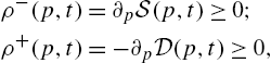
In the Walrasian theory, supply and demand pre-exist and the Walrasian auctioneer gropes (tâtonne) to find the price ptrade![]() that maximizes the amount of possible transactions. The auction then takes place at time t and removes instantly all matched orders. Assuming that all the supply and demand intentions close to the transaction price were revealed before the auction and were matched, the state of the MSD just after the auction is simple to describe, see Fig. 5:
that maximizes the amount of possible transactions. The auction then takes place at time t and removes instantly all matched orders. Assuming that all the supply and demand intentions close to the transaction price were revealed before the auction and were matched, the state of the MSD just after the auction is simple to describe, see Fig. 5:
(19) {ρ−(p,t+)=ρ−(p,t−)(p>ptrade)ρ−(p,t+)=0(p⩽ptrade)ρ+(p,t+)=ρ+(p,t−)(p<ptrade)ρ+(p,t+)=0(p⩾ptrade).

Now what happens next, once the auction has been settled? The aim of this section is to set up a plausible framework for the dynamics of the supply and demand curves. This will allow us to describe, among other questions, how the supply and demand curves evolve from the truncated shape given by Eq. (19) up to the next auction at time t+τ![]() .
.

6.1.2 General Hypotheses About the Behavior of Agents
The theoretical framework presented here relies on general assumptions on the behavior of market agents, that generalize in one crucial way the Santa-Fe model and its extension presented above: agents can update continuously their valuation and correspondingly change their position in the latent limit order book. The resulting equations lead, in certain limits, to a universal evolution of the MSD curves with only two relevant parameters: the price volatility, and the market activity (traded volume per unit time).
We will assume that market participants only have a partial knowledge of the “fundamental” price process, which they try to estimate each in their own way, i.e. with some idiosyncratic error around a certain reference price pF(t)![]() . In the absence of transactions, the MSD curves evolve according to three distinct mechanisms, that we model as follows:
. In the absence of transactions, the MSD curves evolve according to three distinct mechanisms, that we model as follows:
- 1. New intentions: Intentions to buy/sell, not present in the MSD before time t, can appear. The probability for new buy/sell intentions to appear between t and t+dt
 and between prices p and p+dp
 is given by λ±(p−pF(t))dpdt
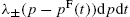 , where λ+(x)
 is a decreasing function of x and λ−(x)
 is an increasing function of x. This is similar to the deposition rate in the Santa Fe model, except that the λ's are centered around the reference price pF(t)
 and not the current mid-price.
 - 2. Cancellations: Already existing intentions to buy/sell at price p can simply be canceled and disappear from the supply and demand curves. The probability for an existing buy/sell intention around price p to disappear between t and t+dt is chosen to be ν±(p−pF(t))dt
 .
. - 3. Price revisions: Already existing intentions to buy/sell at price p can be revised, because of e.g. new information, or because of idiosyncratic factors. We assume that between t and t+dt, each agent i revises his/her reservation price pit
 as
as
(20) pit⟶pit+βitdξt+dWit,
- where dξt
 is common to all i, representing some public information, while βit
 is the sensitivity of agent i to the news, which we imagine to be a random variable with a mean normalized such that Ei[βit]=1
 . Some agents may over-react (βit>1
 ), others under-react (βit<1
 ). The idiosyncratic contribution dWit
 is an independent Wiener noise both across different agents and in time, with distribution of mean zero and variance Σ2dt
 which we take for simplicity independent of i (but some agents could be more “noisy” than others). Both the variation of βit across agents, and the noise contribution dWit reflect the heterogeneity of agents' beliefs.
For simplicity, the “news” term dξt![]() is chosen to a Wiener noise of variance σ2dt
is chosen to a Wiener noise of variance σ2dt![]() . Normalizing the mean of the βit
. Normalizing the mean of the βit![]() 's to unity thus corresponds to the assumption that agents are on average unbiased in their interpretation of the news – i.e. their intentions remain centered around the fundamental price pF(t)=∫tdξt′
's to unity thus corresponds to the assumption that agents are on average unbiased in their interpretation of the news – i.e. their intentions remain centered around the fundamental price pF(t)=∫tdξt′![]() .
.
One final assumption is that the idiosyncratic behavior does “average out” in the limit of a very large number of agents, i.e., that no single market participant accounts for a finite fraction of the total supply or demand. This assumption leads to a deterministic aggregate behavior and allows one to gloss over some rather involved mathematics.
Note the similarities and differences with the Santa Fe model for the LOB, see Section 4. In the Santa Fe model, orders appear and get canceled with Poisson rates, much as postulated above for the latent supply and demand curves. However, the price revision process – with the common news driver dξt![]() – is absent from the Santa Fe model. In other words, while the dynamics of the price is fully explained by the order flow in the Santa Fe model, the present specification allows one to include some exogenous factors as well.
– is absent from the Santa Fe model. In other words, while the dynamics of the price is fully explained by the order flow in the Santa Fe model, the present specification allows one to include some exogenous factors as well.
6.1.3 The “Free Evolution” Equation for MSD Curves
Endowed with the above hypothesis, one can obtain stochastic partial differential equations for the evolution of the average marginal supply (ρ−(p,t)=∂pS(p,t)![]() ) and the average marginal demand (ρ+(p,t)=−∂pD(p,t)
) and the average marginal demand (ρ+(p,t)=−∂pD(p,t)![]() ) in the absence of transactions. The derivation of these equations in beyond the scope of this chapter; their final form is however quite intuitive and easy to interpret – see Mastromatteo et al. (2014b), Donier et al. (2015).8 It turns out that these equations take a simple form in the moving frame of the reference price pF(t)
) in the absence of transactions. The derivation of these equations in beyond the scope of this chapter; their final form is however quite intuitive and easy to interpret – see Mastromatteo et al. (2014b), Donier et al. (2015).8 It turns out that these equations take a simple form in the moving frame of the reference price pF(t)![]() . Introducing the shifted price x=p−pF(t)
. Introducing the shifted price x=p−pF(t)![]() , one finds:
, one finds:
(21) {∂tρ+(x,t)=D∂2xxρ+(x,t)−ν+(x)ρ+(x,t)+λ+(x);∂tρ−(x,t)=D∂2yyρ−(x,t)︸Revisions−ν−(x)ρ−(x,t)︸Cancellations+λ−(x)︸New orders,

where the three terms have a rather transparent origin. The diffusion coefficient D is given by (Σ2+σ2V[βit])/2![]() , i.e. part of the diffusion comes from the purely idiosyncratic “noisy” updates of agents (Σ2
, i.e. part of the diffusion comes from the purely idiosyncratic “noisy” updates of agents (Σ2![]() ), and another part comes from the inhomogeneity of their reaction to news (σ2V[βit]
), and another part comes from the inhomogeneity of their reaction to news (σ2V[βit]![]() ), which indeed vanishes if all βii
), which indeed vanishes if all βii![]() 's are equal to unity. One could argue that extra drift terms should be added to these equations, describing e.g. the propensity of agents to revise their price estimation towards the reference price (x=0
's are equal to unity. One could argue that extra drift terms should be added to these equations, describing e.g. the propensity of agents to revise their price estimation towards the reference price (x=0![]() ). However, these drift terms play a relatively minor role in the following discussion.
). However, these drift terms play a relatively minor role in the following discussion.
Eqs. (21) describe the structural evolution of supply and demand around the reference price pF(t)![]() , which in fact does not appear explicitly in these equations. Interestingly, the dynamics of the MSD curves can be treated independently of the dynamics of the reference price itself, provided one describes the MSD in a moving frame centered around pF(t)
, which in fact does not appear explicitly in these equations. Interestingly, the dynamics of the MSD curves can be treated independently of the dynamics of the reference price itself, provided one describes the MSD in a moving frame centered around pF(t)![]() .
.
Eqs. (21) for ρ+(x,t)![]() and ρ−(x,t)
and ρ−(x,t)![]() are linear and can be formally solved in the general case, starting from an arbitrary initial condition such as Eq. (19). This general solution is however not very illuminating, and we rather focus here in the special case where the cancellation rate ν±(x)≡ν
are linear and can be formally solved in the general case, starting from an arbitrary initial condition such as Eq. (19). This general solution is however not very illuminating, and we rather focus here in the special case where the cancellation rate ν±(x)≡ν![]() does not depend on x nor on the side of the latent order book. The evolution of the MSD can then be written in a transparent way, as
does not depend on x nor on the side of the latent order book. The evolution of the MSD can then be written in a transparent way, as
(22) ρ±(x,t)=∫+∞−∞dx′√4πDtρ±(x′,t=0+)e−(x′−x)24Dt−νt+∫t0dt′∫+∞−∞dx′√4πD(t−t′)λ±(x′)e−(x′−x)24D(t−t′)−ν(t−t′),
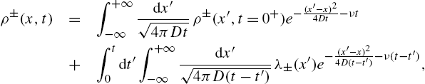
where ρ±(x,t=0+)![]() is the initial condition, i.e. just after the last auction. The first term describes the free evolution of this initial condition, whereas the second term describes new intentions, that appear between time 0 and t.
is the initial condition, i.e. just after the last auction. The first term describes the free evolution of this initial condition, whereas the second term describes new intentions, that appear between time 0 and t.
We will now explore the properties of the above solution at time t=τ−![]() , i.e., just before the next auction, in the two asymptotic limits τ→∞
, i.e., just before the next auction, in the two asymptotic limits τ→∞![]() , corresponding to very infrequent auctions, and τ→0
, corresponding to very infrequent auctions, and τ→0![]() , i.e. continuous time auctions as in modern financial markets. The upshot will be that while the liquidity around the auction price is in general finite and leads to a linear impact, this liquidity vanishes as √τ
, i.e. continuous time auctions as in modern financial markets. The upshot will be that while the liquidity around the auction price is in general finite and leads to a linear impact, this liquidity vanishes as √τ![]() when the inter-auction time τ→0
when the inter-auction time τ→0![]() . This signals the breakdown of linear impact and its replacement by the square-root law detailed in Section 3.2.
. This signals the breakdown of linear impact and its replacement by the square-root law detailed in Section 3.2.
6.2 Infrequent Auctions
The aim of this section is to show that the shape of the marginal supply and demand curves can be characterized in the limit of very infrequent auctions (corresponding to Walras' auctions), allowing one to characterize the famous Kyle impact parameter lambda (Kyle, 1985) in this framework.
Letting t=τ→∞![]() in Eq. (22), one can see that the first term disappears exponentially fast, with rate ν. This means that after time Tm=ν−1
in Eq. (22), one can see that the first term disappears exponentially fast, with rate ν. This means that after time Tm=ν−1![]() , one reaches an equilibrium solution ρ±st.(x)
, one reaches an equilibrium solution ρ±st.(x)![]() , independently of the initial condition. After integrating over t′
, independently of the initial condition. After integrating over t′![]() , the second term can be simplified further to give the following general solution:
, the second term can be simplified further to give the following general solution:
(23) ρ±st.(x)=12√νD∫+∞−∞dx′λ±(x′)e−√νD|x′−x|.
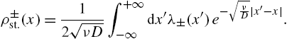
A particularly simple case is when λ±(x)=Ω±e∓x/Δ![]() , meaning that buyers(/sellers) have an exponentially small probability to be interested in a transaction at high/low prices; Δ is the price range within which typically pricing disagreements lie. In this toy-example, one finds that a stationary state only exists when the cancellation rate is strong enough to prevent accumulation of orders far away from x=0
, meaning that buyers(/sellers) have an exponentially small probability to be interested in a transaction at high/low prices; Δ is the price range within which typically pricing disagreements lie. In this toy-example, one finds that a stationary state only exists when the cancellation rate is strong enough to prevent accumulation of orders far away from x=0![]() . When νΔ2>D
. When νΔ2>D![]() , one finds:
, one finds:
ρ±st.(x)=Ω±Δ2νΔ2−De∓x/Δ.
The shape of ρst.(x)![]() is generically the one shown in Fig. 5 with an overlapping region where buy/sell orders coexist. The auction price ptrade=pF+xtrade
is generically the one shown in Fig. 5 with an overlapping region where buy/sell orders coexist. The auction price ptrade=pF+xtrade![]() is determined by the condition (18), or else
is determined by the condition (18), or else
∫∞xtradedxρ+st.(x)=∫xtrade−∞dxρ−st.(x):=Vtrade,
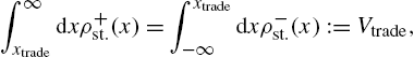
where Vtrade![]() is, by definition, the volume exchanged during the auction. For the simple exponential case above, this equation can be readily solved as
is, by definition, the volume exchanged during the auction. For the simple exponential case above, this equation can be readily solved as
xtrade=Δ2lnΩ+Ω−,
with a clear interpretation: if the new buy order intentions accumulated since the last auction happen to outsize the new sell intentions during the same period, the auction price will exceed the reference price, and vice versa. Would this be the case, one expects the imbalance to invert in the next period (by definition of the reference price), leading to short time mean reversion around pFτ![]() . When Ω+≈Ω−≈Ω0
. When Ω+≈Ω−≈Ω0![]() , one finds:
, one finds:
(24) xtrade≈Ω+−Ω−2Ω0Δ,
and
(25) Vtrade=Ω0Δ3νΔ2−D.
Just after the auction, the MSD curves start again from ρ∓st.(x)![]() , truncated below (resp. above) xtrade
, truncated below (resp. above) xtrade![]() , as in Eq. (19).
, as in Eq. (19).
Let us now turn to price impact in this model, by imagining that a buy metaorder of volume Q is introduced in an otherwise balanced market (i.e. Ω+=Ω−![]() ), with a very high reservation price. For small enough Q's, the clearing price pQ
), with a very high reservation price. For small enough Q's, the clearing price pQ![]() can be computed writing that S(pQ)=D(pQ)+Q
can be computed writing that S(pQ)=D(pQ)+Q![]() and Taylor expanding S(p)
and Taylor expanding S(p)![]() and D(p)
and D(p)![]() around pF
around pF![]() to first order in Q. One readily gets a linear impact law:
to first order in Q. One readily gets a linear impact law:
(26) S(pF)+(pQ−pF)∂pS(pF)=D(pF)+(pQ−pF)∂pD(pF)+Q⇒pQ−pF≈ΛQ

where Kyle's lambda (noted here Λ) is given by
(27) Λ−1=∂pS(pF)−∂pD(pF)=2ρst.(0).
Whenever the MSD do not simultaneously vanish at y=0![]() , the price response to a perturbation must be linear, as in the Kyle model. For the exponential case, one finds:
, the price response to a perturbation must be linear, as in the Kyle model. For the exponential case, one finds:
Λ=Δ2Vtrade,
which has an immediate interpretation: the price impact of a metaorder of volume Q is proportional to the typical mis-pricing Δ times the ratio of Q over the typical transacted volume at each auction Vtrade![]() . Note that for the exponential model, the impact law can be computed beyond the linear regime and reads:
. Note that for the exponential model, the impact law can be computed beyond the linear regime and reads:
(28) I(Q)=pQ−pF=Δsinh−1(Q2Vtrade),

which is linear for small Qs and logarithmic at large Qs.
The main point of the present section is that when the inter-auction time is large enough, each auction clears an equilibrium supply with an equilibrium demand, given by Eq. (23). This corresponds to the standard representation of market dynamics in the Walrasian context, since in this case only the long-term properties of supply and demand matter and the whole transients are discarded. The next section will depart from this limiting case, by introducing a finite inter-auction time such that the transient dynamics of supply and demand becomes a central feature.
6.3 High Frequency Auctions
Let us now investigate the case where the inter-auction time τ tends to zero. Since all the supply (resp. demand) curve left (resp. right) of the auction price is wiped out by the auction process, one expects intuitively that after a very small time τ, the density of buy/sell orders in the immediate vicinity of the transaction price will remain small. We will show that this is indeed the case, and specify exactly the shape of the stationary MSD after many auctions have taken place. Consider again Eq. (22) just before the (n+1)![]() th auction at time (n+1)τ−
th auction at time (n+1)τ−![]() , in the case where the flow of new orders is symmetric, i.e. λ+(x)=λ−(−x)
, in the case where the flow of new orders is symmetric, i.e. λ+(x)=λ−(−x)![]() , such that the transaction price is always at the reference price (xtrade=0
, such that the transaction price is always at the reference price (xtrade=0![]() ). One can focus on the supply side and postulate that ρ−(x,t=nτ−)
). One can focus on the supply side and postulate that ρ−(x,t=nτ−)![]() can be written, in the vicinity of x=0
can be written, in the vicinity of x=0![]() , as
, as
(29) ρ−(x,t=nτ−)=√τϕn(x√Dτ)+O(τ)
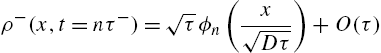
when τ→0![]() . In that limit, one can show that the following iteration equation is exact up to order √τ
. In that limit, one can show that the following iteration equation is exact up to order √τ![]() :
:
(30) ϕn+1(u)=∫+∞0dw√4πϕn(w)e−(u−w)2/4+O(√τ).

Note that ν has entirely disappeared from the equation (but will appear in the boundary condition, see below), and only the value of λ(x)![]() close to the transaction price is relevant at this order.
close to the transaction price is relevant at this order.
After a very large number of auctions, one therefore finds that the stationary shape of the demand curve close to the price and in the limit τ→0![]() is given by the non-trivial solution of the following fixed point equation:
is given by the non-trivial solution of the following fixed point equation:
(31) ϕ∞(u)=∫+∞0dw√4πϕ∞(w)e−(u−w)2/4,
supplemented by the boundary condition ϕ∞(u≫1)≈L√Du![]() , where L
, where L![]() can be fully determined by matching with the explicit solution for τ=0
can be fully determined by matching with the explicit solution for τ=0![]() , leading to
, leading to
(32) L=1D∫∞0dx′[λ(−x′)−λ(x′)]e−√ν/Dx′.
In the exponential model, one finds explicitly:
(33) L=2Ω0ΔΔν−D,
which is a measure of liquidity (see below) that increases with the flux of incoming intentions (Ω0![]() ) and decreases with the cancellation rate ν. Note that L
) and decreases with the cancellation rate ν. Note that L![]() has dimensions of 1/[price]2
has dimensions of 1/[price]2![]() .
.
Eq. (31) is of the so-called Wiener–Hopf type and its analytical solution can be found in e.g. Atkinson (1974). Its numerical solution is found to be very close to an affine function for u>0![]() : ϕ∞(u)≈L√D(u+u0)
: ϕ∞(u)≈L√D(u+u0)![]() with u0≈0.824
with u0≈0.824![]() .
.
In summary, the stationary shape ρst.(x)![]() of the MSD curve in the frequent auction limit τ→0
of the MSD curve in the frequent auction limit τ→0![]() and close to the reference price (x=O(√Dτ)
and close to the reference price (x=O(√Dτ)![]() ), has a universal shape, for a wide class of model specifications (i.e., the functions ν±(x)
), has a universal shape, for a wide class of model specifications (i.e., the functions ν±(x)![]() and λ±(x)
and λ±(x)![]() ). This MSD curve is given by √τϕ∞(x/√Dτ)
). This MSD curve is given by √τϕ∞(x/√Dτ)![]() , where ϕ∞
, where ϕ∞![]() can itself be approximated by a simple affine function. In particular, one finds that the liquidity at the traded price goes to zero as √τ
can itself be approximated by a simple affine function. In particular, one finds that the liquidity at the traded price goes to zero as √τ![]() :
:
(34) ρst.(x=0)≈0.824L√Dτ.
We now turn to the interpretation of this result in terms of market liquidity and price impact. First, one can show that in the τ→0![]() limit, the volume Vtrade
limit, the volume Vtrade![]() cleared at each auction is simply given by
cleared at each auction is simply given by
(35) Vtrade=LDτ.
The total transacted volume VT![]() within a finite time interval of length T is given by VT=VtradeT/τ
within a finite time interval of length T is given by VT=VtradeT/τ![]() . Interestingly, this volume remains finite when τ→0
. Interestingly, this volume remains finite when τ→0![]() , and given by
, and given by
(36) VT=LDT.
This observation should be put in perspective with the recent evolution of financial markets, where the time between transactions τ has indeed become very small, while the volume of each transaction has simultaneously decreased, in such a way that the daily volume has remained roughly constant.
Now, looking back at Eq. (27), one notes that Kyle's Λ behaves as Λ−1≡2ρst.(x=0)∝L√τ![]() , which is the pivotal result of this present section. It means that the marginal supply and demand becomes very small around the transaction price as the auction frequency increases. Intuitively, this is due to the fact that close to the transaction price, liquidity has no time to rebuild between two auctions. From the point of view of price impact, the divergence of Kyle's Λ as 1/√τ
, which is the pivotal result of this present section. It means that the marginal supply and demand becomes very small around the transaction price as the auction frequency increases. Intuitively, this is due to the fact that close to the transaction price, liquidity has no time to rebuild between two auctions. From the point of view of price impact, the divergence of Kyle's Λ as 1/√τ![]() means that the auction price becomes more and more susceptible to any imbalance between supply and demand – as noted in Tóth et al. (2011), the market becomes fragile in the high-frequency limit.
means that the auction price becomes more and more susceptible to any imbalance between supply and demand – as noted in Tóth et al. (2011), the market becomes fragile in the high-frequency limit.
6.4 From Linear to Square-Root Impact
From the shape of the MSD close to transaction price given by Eq. (29), one can compute the supply and demand curves just before an auction, when the inter-auction time τ tends to 0. From these curves one infers the impact of an extra buy order of size Q from the equation
(37) D(pQ)+Q=S(pQ).
Using the results of the previous subsection, one can work out the corresponding impact I(Q)=pQ−pF![]() , with the following result, valid for τ→0
, with the following result, valid for τ→0![]() :
:
(38) I(Q)=√Dτ×Y(QVtrade);Vtrade=LDτ,

where Y(u)![]() is a certain function with the following asymptotic behavior:
is a certain function with the following asymptotic behavior:
(39) Y(u)≈u≪10.555u;Y(u)≈u≫1√2u.
The fact that Y(1)![]() is a number of order unity means that trading the typical auction volume typically moves the price by √Dτ
is a number of order unity means that trading the typical auction volume typically moves the price by √Dτ![]() , i.e. its own volatility on time τ.
, i.e. its own volatility on time τ.
Eq. (38) means that the impact I(Q)![]() is linear in a region where the volume Q is much smaller than Vtrade∼LDτ
is linear in a region where the volume Q is much smaller than Vtrade∼LDτ![]() , i.e. when the extra volume is small compared to the typical volume exchanged during auctions. In the other limit, however, one recovers the square-root impact law analytically:
, i.e. when the extra volume is small compared to the typical volume exchanged during auctions. In the other limit, however, one recovers the square-root impact law analytically:
I(Q≫Vtrade)≈√2QL.

The impact is universal when Q is small enough for the linear approximation of the MSD to hold. For very large Q's, this linear approximation breaks down, and one enters a presumably non-universal regime that is beyond the scope of the present discussion. Impact is Kyle-like for Q<Vtrade![]() and crosses over to a square root regime when Q becomes greater that Vtrade
and crosses over to a square root regime when Q becomes greater that Vtrade![]() . Clearly, for τ→0
. Clearly, for τ→0![]() , the auction volume Vtrade=LDτ
, the auction volume Vtrade=LDτ![]() also tends to zero, so that the region where impact is linear in volume shrinks to zero. In other words, when the market clearing time becomes infinitely small, the impact of small trades is never linear.
also tends to zero, so that the region where impact is linear in volume shrinks to zero. In other words, when the market clearing time becomes infinitely small, the impact of small trades is never linear.
6.5 Summary and Conclusions
The punchline of the above section is quite simple, and well summarized by the graphs plotted in Fig. 5, where we show (a) the standard Walrasian supply and demand curves just before the auction, from which the clearing price ptrade![]() can be deduced; (b) the supply and demand curves just after an auction, when the inter-auction time τ is large enough – in which case the marginal supply and demand are both finite at ptrade
can be deduced; (b) the supply and demand curves just after an auction, when the inter-auction time τ is large enough – in which case the marginal supply and demand are both finite at ptrade![]() ; and (c) the supply and demand curves in the continuous time limit τ→0
; and (c) the supply and demand curves in the continuous time limit τ→0![]() , for which the marginal supply and demand curves vanish linearly around the current price, giving rise to a characteristic V-shaped latent liquidity curve.
, for which the marginal supply and demand curves vanish linearly around the current price, giving rise to a characteristic V-shaped latent liquidity curve.
Remarkably, one can check directly the above prediction on the shape of the MSD curves using Bitcoin data, where traders are much less strategic than in more mature financial markets and display their orders in the visible order book even quite far from the current price. Quite strikingly, the MSD curves are indeed found to be linear in the vicinity of the price that corresponds to about 5% range, in perfect agreement with our dynamical theory of supply and demand in the limit of frequent auctions, see Donier and Bouchaud (2016). Correspondingly, one expects that the impact of meta-orders is well accounted by a square-root law in this region, which is indeed also found empirically (see Donier and Bonart, 2015 for the special case of Bitcoin case).
7 The Information Content of Prices
After the above journey into agent-based, microstructural foundations of price dynamics where fundamental information is completely absent, it is important to discuss one of the most contentious questions in financial economics: what is the real information contained in prices and why do prices move?
7.1 The Efficient Market View
The traditional point of view is that market prices reflect the fundamental value (of a stock, currency, commodity, etc.), up to small and short lived mispricings. Markets are measurement apparatuses that aggregate all private information about the “true” (but hidden) value of assets and provide prices, at the end of a quick and efficient digestion process. Prices are martingales because by definition any new piece of information that changes the value of the asset cannot be anticipated or predicted. In this view, microstructure effects, and trading itself, cannot affect prices except possibly on short time scales. The long term volatility of prices cannot be influenced by short term, microstructural effects.
7.1.1 Three Major Puzzles
This Platonian view of markets is however fraught with several difficulties, that have been the subject of thousands of academic papers in the last 30 years, with renewed insights from microstructure studies. Some of the well-known puzzles are (see Black, 1986 and Shleifer and Summers, 1990 for remarkably clear and lucid early discussions):
- • The excess trading puzzle: If prices really reflect value and are unpredictable, why are there (still) so many people trading? While some amount of excess trading might be justified by risk management or cash management, it is difficult to explain the sheer orders of magnitude of the trading activity in, e.g. stock markets or currency markets.
- • The excess volatility puzzle: Prices move around far too much to be explained by fluctuations of fundamentals (Shiller, 1981). In particular many large price jumps seem to occur without substantial news at all (Cutler et al., 1989; Fair, 2002; Joulin et al., 2008) and, conversely, move much less when markets are closed than when they are open, while the same amount of news continues to be released (French and Roll, 1986).
- • The trend-following puzzle: Price returns tend to be positively autocorrelated on long times scales, such as weeks to months. In other words, some information about future price moves seems to be contained in the past price changes themselves. Trend following appears to be present in all asset classes (including stock indices, commodities, FX, bonds, and so on) and has persisted for at least two centuries, see e.g. Lempérière et al. (2014). This is in stark contradiction with the efficient market story, under which such autocorrelations should not be present. Given that the CTA/trend-following industry managed an estimated 325 billion dollars at the end of 2013, it is hard to argue that these strategies are economically insignificant.
7.1.2 Noise Traders
Faced with the excess volatility/trading puzzles, research in the 80's proposed to break away from the strict orthodoxy of rational market participants and introduce a new category of “noise traders”, or uninformed agents. This, on the one hand, allows one get rid of the “no-trade theorem” and to account for excess trading. As illustrated by the Kyle model or the Glosten–Milgrom model (Kyle, 1985; Glosten and Milgrom, 1985), the existence of noise traders is actually crucial for the viability of market making – and thus of the very existence of markets. However, these models refrain from heresy, in the sense that the long term impact of noise trading on prices is assumed to be zero. Prices still follow fundamental values. This is quite clear in the Kyle model: if the volatility of the fundamental value was zero, the impact of trades would be zero as well. Price impact in this context merely means that trades forecast fundamental prices (Hasbrouck, 2007); but the volatility puzzle is still there since random trades cannot increase volatility.
7.2 Order-Flow Driven Prices
7.2.1 Trades Impact Prices
After accepting the presence of non-rational agents, the next conceptual step is to open the Pandora Box and accept that all trades – informed or random, large or small – do impact prices. This, at least naively, offers a solution to the excess volatility puzzle: if trades by themselves move prices, excess trading should mean excess volatility. We return to this in the next subsection, but note that this view of markets is enticing for several reasons:
- • As we have argued in Section 3, impact is indeed surprisingly large (a metaorder representing 1% of the average daily volume moves the price by ∼10%
 of its average volatility) and long-lived (the impact of an order only decays as a slow, power-law of the lag). Even small, random trades do significantly impact prices.
 - • Because order flow becomes by itself a dominant cause for price changes, market participants should attempt to predict future order flows rather than fundamentals (that may only play a role on much longer time scales). This ties up neatly with Keynes' famous beauty contest:
Investment based on genuine long-term expectation is so difficult [...] as to be scarcely practicable. He who attempts it must surely [...] run greater risks than he who tries to guess better than the crowd how the crowd will behave;
- which is much closer to the way market participants really operate. As reformulated by Shleifer and Summers (1990):
On that view, the key to investment success is not just predicting future fundamentals, but also predicting the movement of other active investors. Market professionals spend considerable resources tracking price trends, volume, short interest, odd lot volume, investor sentiment indexes, and other numerous gauges of demand for equities. Tracking these possible indicators of demand makes no sense if prices responded only to fundamental news and not to investor demand.
- In fact, artificial market experiments show that even when the fundamental value is known to all subjects, they are tempted to forecast the behavior of their fellow subjects and end up creating trends, bubbles, and crashes; see Smith et al. (1988) and Hommes (2013).
- • This scenario allows one to understand why self-exciting, feedback effects are so prevalent in financial markets. As we have seen above, volatility and activity are clustered in time, strongly suggesting that the activity of the market itself leads to more trading which in turn, impact prices and generates more volatility – see Section 2. In fact, calibrating any of these self-exciting models on data lead to the conclusion that the lion's share of the activity/volatility is self-generated, rather than exogenous. In view of Shiller's excess volatility puzzle, this is quite satisfying.
7.2.2 The Statistically Efficient View
There are however at least two potential conundrums with the order-flow dominated theory of price changes.
One is the long-range correlation in order flows (see Section 2.8) that is a clear proof of the presence of long-lived imbalances between supply and demand which markets just cannot quickly digest. These imbalances should create trends and long-lived mispricings. However, we have seen that liquidity providing acts (in normal market conditions) to buffer these imbalances and remove any exploitable price pattern. In other words, competition at the high-frequency end of the spectrum is enough to whiten the time series of returns. Competition enforces a price-setting mechanism whereby liquidity providers/market makers must offer their best guess of future prices based on past order flow. This is essentially the content of the “propagator model” (Bouchaud et al., 2004, 2006) where impact decay, induced by liquidity providers, is fine-tuned to compensate the long-memory of order flow and allow the price to be close to a martingale. In this picture, the volatility of the resulting whitened process is however entirely dominated by high-frequency activity, and has therefore no reason whatsoever to be related to the volatility of the fundamental value. But in fact this is precisely the ingredient we need to account for the excess-volatility puzzle: high-frequency mechanisms set a volatility level that then trickles down unchanged to lower frequencies, generating a trading-induced volatility different from the fundamental volatility.
This is precisely the second conundrum on which many economists immediately pounce. In the words of French and Roll (1986):
Under the trading noise hypothesis, stock returns should be serially correlated [...]: unless market prices are unrelated to the objective economic value of the stock, pricing errors must be corrected in the long run. These corrections would generate negative autocorrelations.
In other words, the (circular) argument is as follows: since in the long-run prices cannot err away from the economic value of the asset, the near-absence of negative autocorrelations is a proof that prices are always close to their fundamental values! The alternative is Black's famous “factor 2” inefficiency (Black, 1986; Bouchaud et al., 2017): prices do err away from their fundamental values by large amounts, and for long times. Back-of-envelope order of magnitude calculations suggest that mean reversion can be as long as a few years, as confirmed by data (Poterba and Summers, 1988; Bouchaud et al., 2017). As pointed out by Summers (1986), this long-term mean reversion hardly leaves any trace that econometricians or traders can exploit.
How can mis-pricing remain for so long, that is, why does the aggregation process that financial markets are supposed to realize fail so badly? One reason often evoked is that the fundamental value is so vaguely determined that the usual arbitrage mechanism – pushing the price back to its fundamental value – is not strong enough (Shleifer and Summers, 1990). Another interesting reason is that self-referential effects can prevent the market as a whole to converge to an unbiased best guess of the fundamental value (Bouchaud, 2013; Bouchaud et al., 2018). Note that in contrast to Kyle's world where the fundamental price is revealed at some time in the future, there is not any terminal time where the “true” level of – say – the S&P500 is announced. While this anchoring does happen at maturity for bond prices or option prices, this idea is not relevant for stock prices or currency levels.
7.2.3 Permanent Impact and Information
If order flow is the dominant cause of price changes, information is chiefly about correctly anticipating the behavior of others and not about fundamental value, as Keynes envisioned. The notion of information should then be replaced by the notion of correlation with future flows. For example, when all market participants interpret a piece of news as negative and trade accordingly, the correct anticipation for an arbitrageur would be to also interpret the news as negative, even if it did not rationally make sense. Of course if all market participants are rational and make trading decision based on their best guess of the fundamental value, order flow will just reflect deviation from fundamentals and the efficient market picture is recovered.
In an order-flow dominated market, the difference between a noise trader and an informed trader is merely the amount of correlation of their trades with the future order flow. Informed traders are positively correlated with it, allowing them to forecast future price changes, whereas noise traders are simply uncorrelated with the rest of the crowd. While the short-term, mechanical impact is similar in both cases (Tóth et al., 2017), on the long run the price reverts to its initial value for noise trades whereas a permanent component remains for “informed” trades. (See Gomes and Waelbroeck, 2014; Donier and Bonart, 2015; Brokmann et al., 2015 for empirical studies on how informed and noise trades impact the price differently on the long run.)
Now, it might well be that even random trades have a non-zero permanent impact – perhaps very small. This is what happens in the Santa-Fe model (see Section 4), while all trades are random, but the rest of the market acts as if they contained some information. This is also the case in Kyle's model when market-makers think there is information when there is none. In the absence of strong anchoring to a fundamental value, the price ends up wandering around because of the order-flow itself, with volatility generated by the price formation mechanism at the microscale.
8 Conclusions and Open Problems
Financial markets display a host of universal “stylized facts” begging for a scientific explanation. The most striking ones, in our eyes, fall into two distinct categories:
- • Excess volatility, fat tails, and clustered activity: these ubiquitous observations strongly suggest that strong self-exciting effects or positive feedback loops are at play. Although mathematical models such as GARCH or Hawkes processes explicitly describe such feedback effects, it is fair to say that there is at this stage no deep understanding of their “microscopic” origin.
- • Order flow regularities, such as the long memory of the sign of market orders or the square-root impact of metaorders.
Agent-based models are attempts to account for these stylized facts in a unified manner. Devising faithful microstructural ABMs would allow one to answer crucial questions, such as those related to market stability. Can large metaorders destabilize markets? Is HFT activity detrimental? Can crashes be endogenously generated and can destabilizing feedback loops be mitigated by adequate regulation?
We have reviewed above some of the recent work in that direction. We have seen in Section 4 that the Santa-Fe zero-intelligence model offers a very interesting benchmark, but suffers from important drawbacks as well, in particular when one wants to use it to account for the square-root impact of metaorders, that requires long memory times for the underlying (latent) liquidity. In its original version, the Santa-Fe model with a long memory time leads to strong mean-reversion effects for the price, which are not observed. A way out of this conundrum is to enrich the Santa-Fe model by allowing market order signs to be autocorrelated – as empirically observed – and to adapt their volume to the available volume on the opposite side. This model is able to reproduce both a diffusive price, and the square-root dependence of the impact on the volume of metaorders (see Section 5). The underlying mechanism can be well understood in terms of a generic “reaction–diffusion” model for the dynamics of the liquidity (see Section 6), that allows one to derive the square-root law analytically in the limit of continuous time auctions (Mastromatteo et al., 2014b; Donier et al., 2015; Donier and Bouchaud, 2016). In a nutshell, a diffusive price leads to a vanishing liquidity in the vicinity of the current price. This naturally accounts for the fact that large metaorders have to be fragmented in order to be digested by the liquidity funnel, which leads to a long memory in the sign of the order flow. Second, the anomalously small local liquidity induces a breakdown of the linear impact model and its replacement by a square-root law.
Although the square-root impact is well reproduced, many open problems remain. One is the relevance of an “information-less” description of financial markets, where prices move around merely as a result of random trades, without any of the usual assumptions about the rationality of agents, the anchoring to fundamental prices through arbitrage, etc. We have argued in Section 7 that the role of information is probably overstated in classical theories, while a picture based on a self-reflexive price-impacting order flow has many merits. Although still hotly debated, this point of view has a strong tradition, going back to Keynes, followed by Shiller, Black, Summers, and others (see Black, 1986; Shleifer and Summers, 1990; Farmer and Geanakoplos, 2009 for inspiring pieces; and Bouchaud et al., 2017 for a recent discussion). The recent accumulation of microstructural stylized facts, allowing one to focus on the price formation mechanism, all but confirm that fundamental information plays a relatively minor role in the dynamics of financial markets, at least on short to medium time scales.
Related to this discussion, a particularly important question is to understand the mechanisms leading to price jumps, which seem to be mostly of endogenous origin and not to news affecting fundamental factors (Cutler et al., 1989; Fair, 2002; Joulin et al., 2008). The order flow driven picture may offer a way to understand why the structure of price jumps is so similar across all traded, liquid markets and all epochs. How might this idea be implemented within the ABM's considered in this chapter, which do not generate fat-tail distributions?9
Here, we offer a conjecture, that obviously requires further scrutiny. In Section 5, we have assumed that latent orders instantaneously materialize in the real order book as the distance to the price gets small. However, any finite conversion time or increased cancellation rates might induce liquidity droughts. These are usually and self-heal rapidly, but they can amplify when price changes accelerate and lead to an unstable feedback loop (Bouchaud, 2011; Fosset et al., 2018). The anomalously low liquidity in the vicinity of the traded price, suggested by the arguments in Section 6, surely contributes to the appearance of these micro-crises, that can eventually become macro-crashes. This simple mechanism could explain the universal power-law distribution of returns that appear to be unrelated to exogenous news but rather to unavoidable, self-induced liquidity crises. Whether this scenario is realized in real markets remains to be vindicated.
Acknowledgements
I want to thank all my collaborators for sharing their precious insights on these issues: M. Benzaquen, G. Bormetti, F. Caccioli, J. De Lataillade, Z. Eisler, J.D. Farmer, A. Fosset, S. Gualdi, J. Kockelkoren, Y. Lempérière, F. Lillo, I. Mastromatteo, F. Patzelt, M. Potters, D. Taranto, B. Tóth. Special thanks to J. Bonart, J. Donier, and M. Gould, with whom a substantial part of the present material was elaborated (see Bouchaud et al., 2018). I also want to thank C. Hommes and B. LeBaron for giving me the opportunity to write this review piece.