
Heterogeneous Agent Models in Finance✶
Roberto Dieci⁎; Xue-Zhong He†,1 ⁎University of Bologna, Bologna, Italy
†University of Technology Sydney, Sydney, NSW, Australia
1Corresponding author. email address: [email protected]
Abstract
This chapter surveys the state-of-art of heterogeneous agent models (HAMs) in finance using a jointly theoretical and empirical analysis, combined with numerical analysis from the latest development in computational finance. It provides supporting evidence on the explanatory power of HAMs to various stylized facts and market anomalies through model calibration, estimation, and economic mechanisms analysis. It presents HAMs with the mainstream finance a unified framework in continuous time to study the impact of historical price information on price dynamics, profitability and optimality of fundamental and momentum trading. It demonstrates how HAMs can help to understand stock price co-movements and evolutionary CAPM. It also introduces a new HAMs perspective on house price dynamics and an integrate approach to study dynamics of limit order markets. The survey provides further insights into the complexity and efficiency of financial markets and policy implications.
Keywords
Heterogeneity; Bounded rationality; Heterogeneous agent-based models; Stylized facts; Asset pricing; Housing bubbles; Limit order markets; Information efficiency; Comovement
1 Introduction
Economic and finance theory is witnessing a paradigm shift from a representative agent with rational expectations to boundedly rational agents with heterogeneous expectations. This shift reflects a growing evidence on the theoretical limitations and empirical challenges in the traditional view of homogeneity and perfect rationality in finance and economics.
The existence of limitations to fully rational behavior and the roles of psychological phenomena and behavioral factors in individuals' decision making have been emphasized and discussed from a variety of different standpoints in the economics and finance literature (see, e.g. Simon, 1982, Sargent, 1993, Arthur, 1994, Conlisk, 1996, Rubinstein, 1998, and Shefrin, 2005). Due to endogenous uncertainty about the state of the world and limits to information and computational ability, agents are prevented from forming rational forecasts and solving life-time optimization problems. Rather, agents favor simple reasoning and ‘rules of thumb’, such as the well documented technical analysis and active trading from financial market professionals.1 In addition, empirical investigations of financial time series show a number of market phenomena (including bubbles, crashes, short-run momentum and long-run mean reverting in asset prices) and some common features, the so-called stylized facts,2 which are difficult to accommodate and explain within the standard paradigm based on homogeneous agents and rational expectations.
Moreover, agents are heterogeneous in their beliefs and behavioral rules, which may change over time due to social interaction and evolutionary selection (see Lux, 1995, Arthur et al., 1997b, and Brock and Hommes, 1998). Such heterogeneity and diversity in individual behavior in economics, along with social interaction among individuals, can hardly be captured by a ‘representative’ agent at the aggregate level (see Kirman, 1992, 2010 for extensive discussions). For instance, as Heckman (2001), the 2000 Nobel Laureate in Economics, points out (concerning the contribution of microeconometrics to economic theory), “the most important discovery was the evidence on pervasiveness of heterogeneity and diversity in economic life. When a full analysis was made of heterogeneity in response, a variety of candidate averages emerged to describe the average person, and the longstanding edifice of the representative consumer was shown to lack empirical support.” Regarding agents' behavior during crisis periods and the role of policy makers, the former ECB president Jean-Claude Trichet writes “We need to deal better with heterogeneity across agents and the interaction among those heterogeneous agents”, highlighting the potential of alternative approaches such as behavioral economics and agent-based modeling.
Over the last three decades, empirical evidence, unconvincing justification of the assumption of unbounded rationality, and role of investor psychology have led to an incorporation of heterogeneity in beliefs and bounded rationality of agents into financial market modeling and asset pricing theory. This has changed the landscape of finance theory dramatically and led to fruitful development in financial economics, empirical finance, and market practice. In this chapter, we focus on the state-of-the-art of this expanding research field, denoted as Heterogeneous Agent Models (HAMs) in finance.
HAMs start from the contributions of Day and Huang (1990), Chiarella (1992), de Grauwe et al. (1993), Lux (1995), Brock and Hommes (1998), inspired by the pioneering work of Zeeman (1974) and Beja and Goldman (1980). This modeling framework views financial market dynamics as a result of the interaction of heterogeneous investors with different behavioral rules, such as fundamental and technical trading rules. One of the key aspects of these models is the expectation feedback mechanism. Namely, agents' decisions are based upon the predictions of endogenous variables whose actual values are determined by the expectations of agents. This results in the co-evolution of beliefs and asset prices over time. Earlier HAMs develop various nonlinear models to characterize various endogenous mechanisms of market fluctuations and financial crisis resulting from the interaction of heterogeneous agents rather than exogenous shocks or news. Overall, such models demonstrate that asset price fluctuations can be caused endogenously. We refer to Hommes (2006), LeBaron (2006), Chiarella et al. (2009a), Hommes and Wagener (2009), Westerhoff (2009), Chen et al. (2012), Hommes (2013), and He (2014) for surveys of these developments in the literature.
HAMs have strong connections with a broader area of Agent-Based Models (ABMs) and Agent-based Computational Economics (ACE). In fact, HAMs can be regarded as particular types of ABMs. However, generally speaking, ABMs are by nature very computationally oriented and allow for a large number of interacting agents, network structures, many parameters, and thorough descriptions of the underlying market microstructures. As such, they turn out to be extremely flexible and powerful, suitable for simulation, scenario analysis and regulation of real-world dynamic systems (see, e.g. Tesfatsion and Judd, 2006, LeBaron and Tesfatsion, 2008). By contrast, HAMs are typically characterized by substantial simplifications at the modeling level (few belief-types or behavioral rules, simplified interaction structures and reduced number of parameters). This makes HAMs analytically tractable to some extent, mostly within the theoretical framework of nonlinear dynamical systems. However, unlike computationally oriented ABMs, HAMs allow a deeper understanding of the basic dynamic mechanisms and driving forces at work, making it possible to identify different and clear-cut ‘types’ of macro outcomes in connection to specific agents' behavior.
Among the large number of HAMs in finance, this chapter is mostly concerned with analytically tractable models based on the interplay of two broad types of beliefs: extrapolative vs. regressive (or technical vs. fundamental rules, or chartists vs. fundamentalists). Since chartists rely on extrapolative rules to forecast future prices and to take their position in the market, they tend to sustain and reinforce current price trends or to amplify the deviations from the ‘fundamental price’. By contrast, fundamentalists place their orders in view of a mean reversion of asset price to its fundamental in long-run. The interplay between such forces is able to capture, albeit in a simplified manner, a basic mechanism of price fluctuations in financial markets. Support to this kind of behavioral heterogeneity comes from survey evidence (Menkhoff and Taylor, 2007, Menkhoff, 2010), experimental evidence (Hommes et al., 2005, Heemeijer et al., 2009), and empirically grounded discussion on the profitability of momentum and mean reversion strategies in financial markets (e.g. Lakonishok et al., 1994, Jegadeesh and Titman, 2001, Moskowitz et al., 2012).
In this chapter, we focus on the state-of-the-art of HAMs in finance from five main strands of the literature developed approximately over the last ten years since the appearance of the previous contributions in Volume II of this Handbook series. This development can have profound consequences for the interpretation of empirical evidence and the formulation of economic policy.
The first strand of research (Section 2) emphasizes the lasting potential of stylized HAMs in discrete time (in particular, chartist-fundamentalist models) to address key issues in finance. Such models have been largely investigated in the past in a wide range of versions incorporating heterogeneity, adaptation, evolution, and even learning (Hommes, 2001, Chiarella and He, 2002, 2003, and Chiarella et al., 2002, 2006b). They have successfully explained various market behavior, such as the long-term swing of market prices from fundamental price, asset bubbles, and market crashes, showing a potential to characterize and explain the stylized facts (Alfarano et al., 2005, Gaunersdorfer and Hommes, 2007) and various power law behavior (He and Li, 2008 and Lux and Alfarano, 2016) observed in financial markets. In addition, the chartist-fundamentalist framework can still provide insight into various stylized facts and market anomalies, and relate them to the economic mechanisms, parameters and scenarios of the underlying nonlinear deterministic systems. Such promising perspectives have motivated further empirical studies, leading to a growing literature on the calibration and estimation of the HAMs. In particular, in Sections 2.1 and 2.2, we focus on a simple HAM of Dieci et al. (2006) to illustrate its explanatory power to volatility clustering through calibration and empirical estimation, and relate the results to the underlying mechanisms and bifurcations of the nonlinear deterministic ‘skeleton’. Moreover, by considering an integrated approach of HAMs and incomplete information about the fundamental value, we provide a micro-foundation to the endogenous trading heterogeneity and switching behavior wildly characterized in HAMs (Section 2.3). We also survey fund flow effect among competing and evolving investment strategies (Section 2.4).
The second strand (Section 3) is on the development of a general framework in continuous time HAMs to incorporate historical price information in the HAMs. It provides a plausible way to deal with a variety of expectation rules formed from historical prices via moving averages over different time horizons, through a parsimonious system of stochastic delay differential equations. We introduce a time delay parameter to measure the effect of historical price information. Besides being consistent with continuous-time finance, this framework appears promising to understand the impact on market stability of lagged information (incorporated in different moving average rules and in realized profits recorded over different time horizons) and to explain a number of phenomena, particularly the long-range dependence in financial markets. We illustrate this approach and the main results in Section 3.1 by surveying the model in He and Li (2012). We emphasize the similarities to and differences from discrete-time HAMs. Moreover, Sections 3.2 and 3.3 demonstrate how useful the continuous-time HAMs can be in addressing the profitability of momentum and contrarian strategies and the optimal allocation with time series momentum and reversal, two of the most dominating financial market anomalies.
The third strand (Section 4) is on the impact of heterogeneous beliefs, expectations feedback and portfolio diversification on the joint dynamics of prices and returns of multiple risky assets. A related issue concerns the joint dynamics of international asset markets, driven by heterogeneous speculators who switch across markets depending on relative profit opportunities. In such models, often described by dynamical systems of large dimension, the typical nonlinear features of baseline HAMs interact with additional nonlinearities that arise naturally within a multi-asset setting, such as the beliefs about second moments and correlations. Section 4 surveys such models, starting from the basic setup developed by Westerhoff (2004), in which investors can switch not only across strategies but across markets (Section 4.1). Such models are not only able to reproduce various stylized facts, but also to offer some explanations to price comovements and cross-correlations of volatilities reported empirically (Schmitt and Westerhoff, 2014), as well as to address some key regulatory issues (Westerhoff and Dieci, 2006). Further research deals with asset comovements and changes in correlations from a different perspective. Based on models of evolving beliefs and (mean-variance) portfolios of heterogeneous investors, Section 4.2 is devoted to the multi-asset HAM of Chiarella et al. (2013b). This approach appears quite promising to address the issue of ‘time-varying betas’ within an evolutionary CAPM framework. It establishes a link between investors' behavior and changes in risk-return relationships at the aggregate level. Finally, Section 4.3 applies HAMs to illustrate the potentially destabilizing impact of the interlinkages between stock and foreign exchange markets (Dieci and Westerhoff, 2010, 2013b).
The fourth strand (Section 5) investigates the dynamics of house prices from the perspective of HAMs. Similar to financial markets, housing markets have long been characterized by boom-bust cycles and other phenomena apparently unrelated to changes in economic fundamentals, such as short-term positive autocorrelation and long-term mean-reversion, which are at odds with the predictions of the rational representative agent framework. Moreover, peculiar features of the housing market (such as the ‘twofold’ nature of housing, illiquidity, and supply-side elasticity) may interact with investors' demand influenced by behavioral factors. Section 5.1 surveys two recent HAMs of the housing market (Bolt et al., 2014 and Dieci and Westerhoff, 2016) which are based on mean-variance preferences and standard equilibrium conditions, with the fundamental price being regarded as the present value of future expected rental payments. However, within this framework, investors form heterogeneous expectations about future house prices, according to (evolving) regressive and extrapolative beliefs. Estimation of similar models supports the assumption of behavioral heterogeneity changing over time, based on the relative performance of the competing prediction rules. It highlights how such heterogeneity can produce endogenous house price bubbles and crashes (disconnected from the dynamics of the fundamental price). Moreover, the nonlinear dynamic analysis of such models can provide a simple behavioral explanation for the observed role of supply elasticity in ‘shaping’ housing bubbles and crashes, as widely reported and discussed in empirical and theoretical literature (see, e.g. Glaeser et al., 2008). Further ‘disequilibrium’ models, illustrated in Section 5.2, confirm the main findings about the impact of behavioral heterogeneity on housing price dynamics.
The fifth strand (Section 6) is on an integrated approach combining HAMs with traditional market microstructure literature to examine the joint impact of information asymmetry, heterogeneous expectations, and adaptive learning in limit order markets. As shown in Section 6.1, these HAMs are very helpful in examining complexity in market microstructure, providing insight into the impact of heterogeneous trading rules on limit order book and order flows (Chiarella and Iori, 2002, Chiarella et al., 2009b, 2012b, Kovaleva and Iori, 2014), and replicating the stylized facts in limit order markets (Chiarella et al., 2017). Earlier HAMs mainly examine the endogenous mechanism of interaction of heterogeneous agents, less so about information asymmetry, which is the focus of traditional market microstructure literature under rational expectations. Moreover, while the current microstructure literature focuses on informed traders by simplifying the behavior of uninformed traders substantially, a thorough modeling of the learning behavior of uninformed traders appears crucial for trading and market liquidity (O'Hara, 2001). Section 6.2 surveys a contribution in this direction by Chiarella et al. (2015a). By integrating HAMs with asymmetric information and Genetic Algorithm (GA) learning into microstructure literature, they examine the impact of learning on order submission, market liquidity, and price discovery. Finally, very recent contributions (in Sections 6.3 and 6.4) further examine the impact of high frequency trading (Arifovic et al., 2016) and different regulations (Lensberg et al., 2015) on market in a GA learning environment.
Most of the development surveyed in this chapter is based on a jointly theoretical and empirical analysis, combined with numerical simulations and Monte Carlo analysis from the latest development in computational finance. It provides very rich approaches to deal with various issues in equity market, housing market, and market microstructure. The results provide some insights into our understanding of the complexity and efficiency of financial market and policy implications.
2 HAMs of Single Asset Market in Discrete-Time
Empirical evidence of various stylized facts and anomalies in financial markets, such as fat tails in return distribution, long-range dependence in volatility, and time series momentum and reversal, has stimulated increasing research interest in financial market modeling. By focusing on endogenous heterogeneity of investor behavior, HAMs play a very important role in providing insights into the importance of investor heterogeneity and explaining stylized facts and marker anomalies observed in financial time series. Early HAMs consider two types of traders, typically fundamentalists and chartists. Beja and Goldman (1980), Day and Huang (1990), Chiarella (1992), Lux (1995), and Brock and Hommes (1997, 1998) are amongst the first to have shown that interaction of agents with heterogeneous expectations can lead to market instability. These HAMs have successfully explained market booms, crashes, and the deviations of market price from fundamental price and replicated some of the stylized facts, which are nicely surveyed in Hommes (2006), LeBaron (2006), and Chiarella et al. (2009a). The promising perspectives of HAMs have stimulated further studies on empirical testing in different markets, including commodity markets (Baak, 1999, Chavas, 2000), stock markets (Boswijk et al., 2007; Franke, 2009; Franke and Westerhoff, 2011, 2012; Chiarella et al., 2012a, 2014; He and Li, 2015a, 2015b), foreign exchange markets (Westerhoff and Reitz, 2003; de Jong et al., 2010; ter Ellen et al., 2013), mutual funds (Gomes and Michaelides, 2008), option markets (Frijns et al., 2010), oil markets (ter Ellen and Zwinkels, 2010), and CDS markets (Chiarella et al., 2015b). HAMs have also been estimated with contagious interpersonal communication by Gilli and Winker (2003), Alfarano et al. (2005), Lux (2009a, 2012), and other works reviewed in Chen et al. (2012).
This development has spurred recent attempts at theoretical explanations and the underlying economic mechanism analysis, which is nicely summarized in a recent survey of Lux and Alfarano (2016). Several behavioral mechanisms on volatility clustering have been proposed based on the underlying deterministic dynamics (He and Li, 2007, 2015b, 2017, Gaunersdorfer et al., 2008, He et al., 2016b), stochastic herding (Alfarano et al., 2005), and stochastic demand (Franke and Westerhoff, 2011, 2012).
In this section, we use the simple HAM of Dieci et al. (2006) to illustrate the explanatory power of the model to investor behavior and provide some of the underlying mathematical and economic mechanisms to volatility clustering and long-range dependence in volatility. We first introduce the model of boundedly rational and adaptive switching behavior of investors in financial markets in Section 2.1. We then provide two particular mechanisms to explain volatility clustering and long memory in return volatility based on the underlying deterministic dynamics in Section 2.2. Mathematically, the first is based on the local stability and Hopf bifurcation, explored in He and Li (2007), while the second is characterized by the coexistence of two locally stable attractors with different size, proposed initially in Gaunersdorfer et al. (2008) and further developed theoretically in He et al. (2016b). Economically, it demonstrates that the dominance of trend chasing behavior when investors cannot change their strategies or the intensive switching behavior of investors to switch to more profitable strategy can explain volatility clustering and long memory in return volatility, while the noise traders also play a very important role.
In Section 2.3, we briefly discuss He and Zheng (2016) about the emergence of trading heterogeneity due to information uncertainty and strategic trading of agents. Through an integrated approach of HAMs and incomplete information about the fundamental value, He and Zheng (2016) provide an endogenous self-correction mechanism of the market. This mechanism is very different from the HAMs with complete information, in which mean-reverting is channeled through some kind of nonlinear assumptions on the demand or order flow of risky asset and market stability depends exogenously on balanced activities from fundamental and momentum trading. The approach provides a micro-foundation to endogenous trading heterogeneity and switching behavior wildly characterized in HAMs. We complete the section with a discussion about an evolutionary finance framework in Section 2.4 to examine the effect of the flows of funds among competing and evolving investment styles on investment performance.
2.1 Market Mood and Adaptive Behavior
Empirical evidence in foreign exchange markets (Allen and Taylor, 1990, Taylor and Allen, 1992, Menkhoff, 1998, and Cheung et al., 2004) and managing fund industrial (Menkhoff, 2010) suggests that agents have different information and/or beliefs about market processes. They use not only fundamental but also technical analyses, which are consistent with short-run momentum and long-run reversal behavior in financial markets. In addition, although some agents do not change their particular trading strategies, there are agents who may switch to more profitable strategies over time. Recent laboratory experiments in Hommes et al. (2005), Anufriev and Hommes (2012), and Hommes and in't Veld (2015) also show that agents using simple “rule of thumb” trading strategies are able to coordinate on a common prediction rule. Therefore heterogeneity in expectations and adaptive behavior are crucial to describe individual forecasting and aggregate price behavior.
Motivated by the empirical and experiment evidence, Dieci et al. (2006) introduce a simple financial market of fundamentalists and trend followers. Some agents switch between different strategies over time according to their performance, characterizing the adaptively rational behavior of agents. Others are confident and stay with their strategies over time, representing market mood. It turns out that this simple model is rich enough to illustrating the complicated price dynamics and to exploring different mechanisms in generating volatility clustering and long memory in volatility. In the following, we first outline the model, discuss calibration and empirical estimation of the model, and then provide an analysis on the two underlying mechanisms (see Dieci et al., 2006 and He and Li, 2008, 2017 for the detail).
Consider a financial market with one risky asset and one risk free asset. Let r be the constant risk free rate, pt![]() the price, and dt
the price, and dt![]() the dividend of the risky asset at time t. Assume that there are four types of investors, fundamental traders (or fundamentalists), trend followers (or chartists) and noise traders, and one market maker. Let n3
the dividend of the risky asset at time t. Assume that there are four types of investors, fundamental traders (or fundamentalists), trend followers (or chartists) and noise traders, and one market maker. Let n3![]() be the population fraction of the noise traders. Among 1−n3
be the population fraction of the noise traders. Among 1−n3![]() , the fractions of the fundamentalists and trend followers have fixed, n1
, the fractions of the fundamentalists and trend followers have fixed, n1![]() and n2
and n2![]() , and switching, n1,t
, and switching, n1,t![]() and n2,t=1−n1,t
and n2,t=1−n1,t![]() , components respectively. Denote n0=n1+n2,m0=(n1−n2)/n0
, components respectively. Denote n0=n1+n2,m0=(n1−n2)/n0![]() and mt=n1,t−n2,t
and mt=n1,t−n2,t![]() . Then the market fractions Qh,t
. Then the market fractions Qh,t![]() (h=1,2,3
(h=1,2,3![]() ) of the fundamentalists, trend followers, and noise traders at time t can be rewritten as, respectively,
) of the fundamentalists, trend followers, and noise traders at time t can be rewritten as, respectively,
(1) {Q1,t=12(1−n3)[n0(1+m0)+(1−n0)(1+mt)],Q2,t=12(1−n3)[n0(1−m0)+(1−n0)(1−mt)],Q3,t=n3.

Let Rt+1=pt+1+dt+1−Rpt![]() be the excess return and R=1+r
be the excess return and R=1+r![]() . We model the order flow3 zh,t
. We model the order flow3 zh,t![]() of type-h investors from t to t+1
of type-h investors from t to t+1![]() by zh,t=Eh,t(Rt+1)/(ahVh,t(Rt+1))
by zh,t=Eh,t(Rt+1)/(ahVh,t(Rt+1))![]() , where Eh,t
, where Eh,t![]() and Vh,t
and Vh,t![]() are the conditional expectation and variance at time t and ah
are the conditional expectation and variance at time t and ah![]() is the risk aversion coefficient of type h traders. The order flow of the noise traders ξt∼N(0,σ2ξ)
is the risk aversion coefficient of type h traders. The order flow of the noise traders ξt∼N(0,σ2ξ)![]() is an i.i.d. random variable. Then the population weighted average order flow is given by Ze,t=Q1,tz1,t+Q2,tz2,t+n3ξt.
is an i.i.d. random variable. Then the population weighted average order flow is given by Ze,t=Q1,tz1,t+Q2,tz2,t+n3ξt.![]() To determine the market price, we follow Chiarella and He (2003) and assume that the market price is determined by the market maker as follows,
To determine the market price, we follow Chiarella and He (2003) and assume that the market price is determined by the market maker as follows,
(2) pt+1=pt+λZe,t=pt+μze,t+δt,
where ze,t=q1,tz1,t+q2,tz2,t![]() , qh,t=Qh,t/(1−n3)
, qh,t=Qh,t/(1−n3)![]() for h=1,2
for h=1,2![]() , λ denotes the speed of price adjustment of the market maker, μ=(1−n3)λ
, λ denotes the speed of price adjustment of the market maker, μ=(1−n3)λ![]() and δt∼N(0,σ2δ)
and δt∼N(0,σ2δ)![]() with σδ=λn3σξ
with σδ=λn3σξ![]() .
.
We now describe briefly the heterogeneous beliefs of the fundamentalists and trend followers and the adaptive switching mechanism. The conditional mean and variance for the fundamental traders are assumed to follow
(3) E1,t(pt+1)=pt+(1−α)[Et(p⁎t+1)−pt],V1,t(pt+1)=σ21,
where p⁎t![]() is the fundamental value of the risky asset following a random walk,
is the fundamental value of the risky asset following a random walk,
(4) p⁎t+1=p⁎texp(−σ2ε2+σεεt+1),εt∼N(0,1),σε≥0,p⁎0=p⁎>0,

εt![]() is independent of the noise process δt
is independent of the noise process δt![]() , σ21
, σ21![]() is constant, and hence Et(p⁎t+1)=p⁎t
is constant, and hence Et(p⁎t+1)=p⁎t![]() . Here (1−α)
. Here (1−α)![]() measures the speed of price adjustment towards the fundamental price with 0<α<1
measures the speed of price adjustment towards the fundamental price with 0<α<1![]() . A high α indicates less confidence on the convergence to the fundamental price, leading to a slower adjustment of the market price to the fundamental. For the trend followers, we assume
. A high α indicates less confidence on the convergence to the fundamental price, leading to a slower adjustment of the market price to the fundamental. For the trend followers, we assume
(5) E2,t(pt+1)=pt+γ(pt−ut),V2,t(pt+1)=σ21+b2vt,
where γ⩾0![]() measures the extrapolation of the trend, ut
measures the extrapolation of the trend, ut![]() and vt
and vt![]() are sample mean and variance, respectively. We assume that ut=δut−1+(1−δ)pt
are sample mean and variance, respectively. We assume that ut=δut−1+(1−δ)pt![]() and vt=δvt−1+δ(1−δ)(pt−ut−1)2
and vt=δvt−1+δ(1−δ)(pt−ut−1)2![]() , representing limiting mean and variance of the geometric decay processes when the memory lag tends to infinity. Here δ∈(0,1)
, representing limiting mean and variance of the geometric decay processes when the memory lag tends to infinity. Here δ∈(0,1)![]() measures the geometric decay rate and b2≥0
measures the geometric decay rate and b2≥0![]() measures the sensitivity to the sample variance. For simplicity we assume that investors share a homogeneous belief about the dividend process dt
measures the sensitivity to the sample variance. For simplicity we assume that investors share a homogeneous belief about the dividend process dt![]() , which is i.i.d. and normally distributed with mean ˉd
, which is i.i.d. and normally distributed with mean ˉd![]() and variance σ2d
and variance σ2d![]() . Denote by p⁎=p⁎o=ˉd/r
. Denote by p⁎=p⁎o=ˉd/r![]() the long-run fundamental price.
the long-run fundamental price.
Let πh,t+1![]() be the realized profit between t and t+1
be the realized profit between t and t+1![]() of type-h investors, πh,t+1=zh,t(pt+1+dt+1−Rpt)
of type-h investors, πh,t+1=zh,t(pt+1+dt+1−Rpt)![]() for h=1,2
for h=1,2![]() . Following Brock and Hommes (1997, 1998), the market fraction of investors choosing strategy h at time t+1
. Following Brock and Hommes (1997, 1998), the market fraction of investors choosing strategy h at time t+1![]() is determined by
is determined by
nh,t+1=exp[β(πh,t+1−Ch)]∑iexp[β(πi,t+1−Ci)],h=1,2,
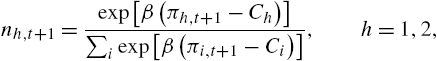
where β measures the intensity of the choice and Ch≥0![]() the cost. Together with (1) the market fractions and asset price dynamics are determined by the following random dynamic system in discrete-time,
the cost. Together with (1) the market fractions and asset price dynamics are determined by the following random dynamic system in discrete-time,
(6) {pt+1=pt+μ(q1,tz1,t+q2,tz2,t)+δt,δt∼N(0,σ2δ),ut=δut−1+(1−δ)pt,vt=δvt−1+δ(1−δ)(pt−ut−1)2,mt=tanh[β2(z1,t−1−z2,t−1−(C1−C2))(pt+dt−Rpt−1)].

2.2 Volatility Clustering: Calibration and Mechanisms
By conducting econometric analysis via Monte Carlo simulations, He and Li (2015b, 2017) show that the autocorrelations of returns, absolute returns and squared returns of the model developed above share the same pattern as those of the DAX 30. They further characterize the power-law behavior of the DAX 30 and find that the estimates of the power-law decay indices, the (FI)GARCH parameters, and the tail index of the model closely match those of the DAX 30. In the following we first report the calibrated results of the model developed in the previous subsection and then provide some insights into investor behavior and two underlying mechanisms of the volatility clustering.
When there is no switching between the two strategies, the above model reduces to the no-switching model in He and Li (2007), showing that the no-switching model is able to replicate the power-law behavior in return volatility. Based on the daily price index data of the DAX 30 from 11 August, 1975 to 29 June, 2007, He and Li (2015b, 2017) calibrate three scenarios of the above model: the no-switching (N) model with β=0![]() , pure-switching (S) model with n0=0
, pure-switching (S) model with n0=0![]() , and full (F) model of (6). The results are collected in Table 1 (with fixed r=5%p.a
, and full (F) model of (6). The results are collected in Table 1 (with fixed r=5%p.a![]() . and C1=C2=0
. and C1=C2=0![]() ). By conducting econometric analysis via Monte Carlo simulations based on the calibrated models, He and Li (2015b, 2017) find that, for all three scenarios, the estimates of the power-law decay indices d, the (FI)GARCH parameters, and the tail index of the calibrated model closely match those of the DAX 30. By conducting a Wald test Ho:dDAX=d
). By conducting econometric analysis via Monte Carlo simulations based on the calibrated models, He and Li (2015b, 2017) find that, for all three scenarios, the estimates of the power-law decay indices d, the (FI)GARCH parameters, and the tail index of the calibrated model closely match those of the DAX 30. By conducting a Wald test Ho:dDAX=d![]() at 5% and 1% significant levels (with the critical values of 3.842 and 6.635, respectively), He and Li (2017) show that switching model fits the data better than the no-switching and pure-switching models.
at 5% and 1% significant levels (with the critical values of 3.842 and 6.635, respectively), He and Li (2017) show that switching model fits the data better than the no-switching and pure-switching models.
Table 1
Calibrated parameters of the no-switching (N), pure-switching (S), and full (F) models
| α | γ | a 1 | a 2 | μ | n 0 | m 0 | δ | b | σ | σ δ | β | Wald | |
|---|---|---|---|---|---|---|---|---|---|---|---|---|---|
| N | 0.858 | 8.464 | 6.024 | 0.383 | 0.946 | 1 | −0.200 | 0.292 | 6.763 | 0.24 | 3.473 | 0 | 112 |
| S | 0.513 | 0.764 | 7.972 | 0.231 | 2.004 | 0 | – | 0.983 | 3.692 | 0.231 | 3.268 | 0.745 | 108 |
| F | 0.488 | 1.978 | 7.298 | 0.320 | 1.866 | 0.313 | −0.024 | 0.983 | 3.537 | 0.231 | 3.205 | 0.954 | 106 |
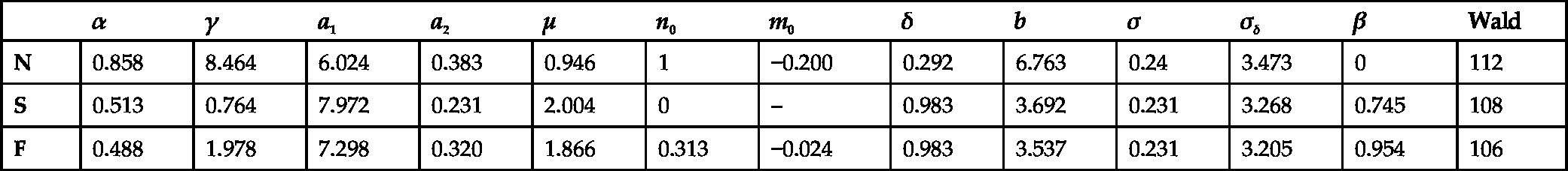
Comparing the estimates of the three scenarios leads to different investor behavior. The estimated annual return volatility σ is close to the annual return volatility of the DAX 30. Higher a1![]() than a2
than a2![]() implies that the fundamentalists are more risk averse compared to the trend followers. For the no-switching scenario, a higher value of α indicates a slow price adjustment of the fundamentalists toward the fundamental value, while a higher value of γ indicates that the trend followers extrapolate the price trend actively. Without switching, mo=−0.2
implies that the fundamentalists are more risk averse compared to the trend followers. For the no-switching scenario, a higher value of α indicates a slow price adjustment of the fundamentalists toward the fundamental value, while a higher value of γ indicates that the trend followers extrapolate the price trend actively. Without switching, mo=−0.2![]() indicates that both the fundamentalists and trend followers are active in the market, which is however dominated by the trend followers (about 60%). On the full model, the market is dominated by investors (about 70%) who constantly switch between the fundamental and trend following strategies, although some investors (about 30%) never change their strategies over the time. This is consistent with the empirical findings discussed at the beginning of this section.
indicates that both the fundamentalists and trend followers are active in the market, which is however dominated by the trend followers (about 60%). On the full model, the market is dominated by investors (about 70%) who constantly switch between the fundamental and trend following strategies, although some investors (about 30%) never change their strategies over the time. This is consistent with the empirical findings discussed at the beginning of this section.
We now provide two mechanisms based on the underlying deterministic dynamics. The first one is on the local stability and periodic oscillation due to Hopf bifurcation, explored in He and Li (2007). Essentially, on the parameter space of the deterministic model, near the Hopf bifurcation boundary, the fundamental steady state can be locally stable but globally unstable. Due to the nature of Hopf bifurcation, such global instability leads to switching between the locally stable fundamental price and the periodic oscillations around the fundamental price. Then triggered by the fundamental and market noises, He and Li (2007) show that the interaction of the fundamental, risk-adjusted trend chasing from the trend followers, and the interplay of the noises and the underlying deterministic dynamics can be the source of power-law behavior in return volatility. Mathematically, the calibrated no-switching and switching models share the same underlying deterministic mechanism. Economically, however, they provide different behavioral mechanisms. With no-switching, it is the dominance of the trend followers (about 60%) that drives the power-law behavior. However, with both switching and no-switching investors, dominated by these traders (about 70%) who constantly switch between the two strategies. It is therefore the adaptive behavior of investors that generates the power-law behavior. This is also in line with Franke and Westerhoff (2012, 2016) who estimate various HAMs and show that herding behavior plays a key role in matching the stylized facts. More importantly, the noise traders play an important role in generating insignificant ACs on the returns, while the significantly decayed AC patterns of the absolute returns and squared returns are more influenced by the fundamental noise. As pointed out in Lux and Alfarano (2016), noise traders is probably a central ingredient of these models.
The second mechanism proposed initially in Gaunersdorfer et al. (2008) is characterized by the coexistence of two locally stable attractors with different size, while such coexistence is not required in the previous mechanism. Dieci et al. (2006) show that the above model can display such co-existence of locally stable fundamental steady state and periodic cycle. The interaction of the coexistence of the deterministic dynamics and the noise processes then triggers the switching among the two attractors and endogenously generates volatility clustering. More recently, by applying normal form analysis and center manifold theory, He et al. (2016b) provide the following theoretical result on the coexistence of the locally stable steady state and invariant circle of the underlying deterministic model (we refer to He et al., 2016b for the details).
Proposition 2.1
The underlying deterministic system of (6) has a unique fundamental steady state (p,u,v,m)=(ˉp,ˉp,0,ˉm)![]() with ˉm=tanhβ(C2−C1)2
with ˉm=tanhβ(C2−C1)2![]() . The fundamental steady state is locally asymptotically stable for γ∈(0,γ⁎⁎)
. The fundamental steady state is locally asymptotically stable for γ∈(0,γ⁎⁎)![]() , and it undergoes a Neimark–Sacker bifurcation at γ=γ⁎⁎
, and it undergoes a Neimark–Sacker bifurcation at γ=γ⁎⁎![]() , that is, there is an invariant curve near the fundamental steady state. Moreover, the bifurcated closed invariant curve is forward and stable when a(0)<0
, that is, there is an invariant curve near the fundamental steady state. Moreover, the bifurcated closed invariant curve is forward and stable when a(0)<0![]() and backward and unstable when a(0)>0
and backward and unstable when a(0)>0![]() , and a Chenciner (generalized Neimark–Sacker) bifurcation takes place when a(0)=0
, and a Chenciner (generalized Neimark–Sacker) bifurcation takes place when a(0)=0![]() . Here a(0)
. Here a(0)![]() is the first Lyapunov coefficient.
is the first Lyapunov coefficient.
Note that the market fractions of the fundamentalists and trend followers at the fundamental steady state are given by q1=(1+mq)/2![]() and q2=(1−mq)/2
and q2=(1−mq)/2![]() with mq=n0m0+(1−n0)ˉm
with mq=n0m0+(1−n0)ˉm![]() , respectively. When the cost of the fundamental strategy C1
, respectively. When the cost of the fundamental strategy C1![]() is higher than the cost of the trend following strategy C2
is higher than the cost of the trend following strategy C2![]() , an increase in the switching intensity β leads to a decrease in γ⁎⁎
, an increase in the switching intensity β leads to a decrease in γ⁎⁎![]() , meaning that the fundamental price becomes less stable when traders switch their strategies more often. This is essentially the rational routes to randomness of Brock and Hommes (1997, 1998).
, meaning that the fundamental price becomes less stable when traders switch their strategies more often. This is essentially the rational routes to randomness of Brock and Hommes (1997, 1998).
Fig. 1 illustrates two different types of Neimark–Sacker bifurcation. It is the sign of the first Lyapunov coefficient a(0)![]() that determines the bifurcation direction, either forward or backward, and the stability of the bifurcated invariant circles, leading to different bifurcation dynamics. When a(0)<0
that determines the bifurcation direction, either forward or backward, and the stability of the bifurcated invariant circles, leading to different bifurcation dynamics. When a(0)<0![]() , the bifurcation is forward and stable, meaning that the bifurcated invariant circle occurring for γ>γ⁎⁎
, the bifurcation is forward and stable, meaning that the bifurcated invariant circle occurring for γ>γ⁎⁎![]() is locally stable. In this case, as γ increases and passes γ⁎⁎
is locally stable. In this case, as γ increases and passes γ⁎⁎![]() , the fundamental steady state becomes unstable and the trajectory converges to an invariant circle bifurcating from the fundamental steady state. As γ increases further, the trajectory converges to invariant circles with different sizes. This is illustrated in Fig. 1A with γ⁎⁎≈0.93
, the fundamental steady state becomes unstable and the trajectory converges to an invariant circle bifurcating from the fundamental steady state. As γ increases further, the trajectory converges to invariant circles with different sizes. This is illustrated in Fig. 1A with γ⁎⁎≈0.93![]() where the two bifurcating curves for γ>γ⁎⁎
where the two bifurcating curves for γ>γ⁎⁎![]() indicate the minimum and maximum value boundaries of the bifurcating invariant circles as γ increases.
indicate the minimum and maximum value boundaries of the bifurcating invariant circles as γ increases.
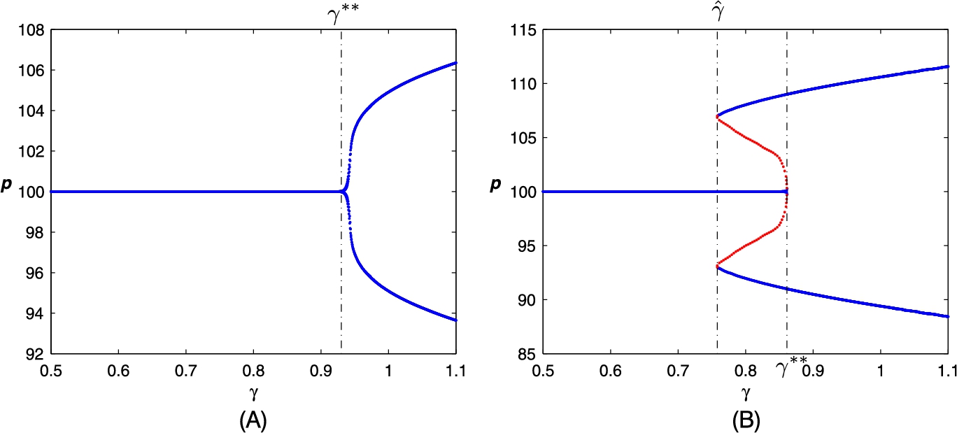
However, when a(0)>0![]() , the bifurcation is backward and unstable, meaning that the bifurcated invariant circle occurring at γ=γ⁎⁎
, the bifurcation is backward and unstable, meaning that the bifurcated invariant circle occurring at γ=γ⁎⁎![]() is unstable, illustrated in Fig. 1B (with γ⁎⁎≈0.88
is unstable, illustrated in Fig. 1B (with γ⁎⁎≈0.88![]() ). There is a continuation of the unstable bifurcated circles as γ decreases initially until it reaches a critical value ˆγ
). There is a continuation of the unstable bifurcated circles as γ decreases initially until it reaches a critical value ˆγ![]() , which is indicated by the two (red) dotted curves of the bifurcating circles for ˆγ<γ<γ⁎⁎
, which is indicated by the two (red) dotted curves of the bifurcating circles for ˆγ<γ<γ⁎⁎![]() . Then as γ increases from the critical value ˆγ
. Then as γ increases from the critical value ˆγ![]() , the bifurcated circles become forward and stable. This is illustrated by the two (blue) solid curves, which are the boundaries of the bifurcating circles, for γ>ˆγ
, the bifurcated circles become forward and stable. This is illustrated by the two (blue) solid curves, which are the boundaries of the bifurcating circles, for γ>ˆγ![]() in Fig. 1B. Therefore, the locally stable steady state coexists with the locally stable ‘forward extended’ circles for ˆγ<γ<γ⁎⁎
in Fig. 1B. Therefore, the locally stable steady state coexists with the locally stable ‘forward extended’ circles for ˆγ<γ<γ⁎⁎![]() , in between there are backward extended unstable circles. For ˆγ<γ<γ⁎⁎
, in between there are backward extended unstable circles. For ˆγ<γ<γ⁎⁎![]() , even when the fundamental steady state is locally stable, prices need not converge to the fundamental value, while may settle down to a stable limit circle. We call ˆγ<γ<γ⁎⁎
, even when the fundamental steady state is locally stable, prices need not converge to the fundamental value, while may settle down to a stable limit circle. We call ˆγ<γ<γ⁎⁎![]() the ‘volatility clustering region’. In addition, a Chenciner (generalized Neimark–Sacker) bifurcation takes place when a(0)=0
the ‘volatility clustering region’. In addition, a Chenciner (generalized Neimark–Sacker) bifurcation takes place when a(0)=0![]() . Based on the above analysis, a necessary condition on the coexistence is that a(0)>0
. Based on the above analysis, a necessary condition on the coexistence is that a(0)>0![]() . The coexistence of the locally stable steady state and invariant circle illustrated in Fig. 2 shows that the price dynamics depends on the initial values.
. The coexistence of the locally stable steady state and invariant circle illustrated in Fig. 2 shows that the price dynamics depends on the initial values.
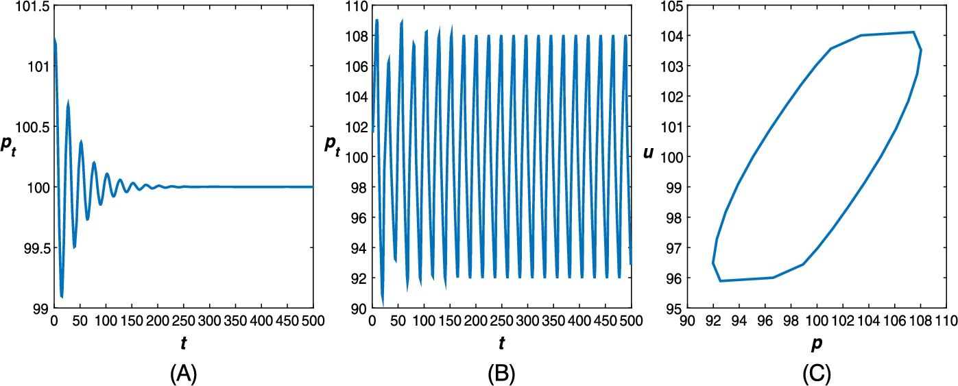
 in (A) and (p0,u0,v0,m0)=(ˉp+1,ˉp−1,0,ˉm)
 in (B) and the phase plot of (p,u) in (C). Here the parameter values are the same as in Fig. 1 and n0 = 0.5. (A) Price time series; (B) price time series; (C) phase plot.
When buffeted with noises, the stochastic model can endogenously generate volatility clustering and long range dependence in volatility, illustrated in Fig. 3. Economically, with strong trading activities of either the fundamental investors or the trend followers, market price fluctuates around either the fundamental value with low volatility or a cyclical price movement with high volatility, depending on market conditions. When the activities of the fundamentalists and trend followers are balanced (to be in the volatility clustering region), the interaction of the fundamental noise and noise traders and the underlying co-existence dynamics then triggers an irregular switching between the two volatility regimes, leading to volatility clustering. In particular, volatility clustering becomes more significant when neither the fundamental nor the trend following traders dominate the market and traders switch their strategies more often. The results verify the endogenous mechanism on volatility clustering proposed by Gaunersdorfer et al. (2008) and provide a behavioral explanation on the volatility clustering.

2.3 Information Uncertainty and Trading Heterogeneity
Traditional finance literature mainly explore the role of asymmetric information and information uncertainty. Most HAMs however mainly focus on endogenous market mechanism through the interaction among heterogeneous agents by assuming a complete information about the fundamental value of risky assets. An integration of HAMs and asymmetric and/or uncertain information would provide a micro-foundation on behavioral heterogeneity and a more broad framework to better explaining various puzzles and anomalies in financial markets. Instead of heuristical heterogeneity assumption of agents' behavior, He and Zheng (2016) model the trading heterogeneity by introducing information uncertainty about the fundamental value to a HAM. Agents are homogeneous ex ante. Conditional on their private information about the fundamental value, agents choose optimally among different trading strategies when optimizing their expected utilities. This approach provides a micro-foundation to trading and behavioral heterogeneity among agents. It also offers a different switching behavior of agents from the current HAMs. In the following, we brief this approach.
Consider a continuum [0,1]![]() of agents trading one risky asset and one risk-free asset in discrete-time. For simplicity, the risk-free rate is normalized to be zero. The fundamental value of the risky asset μ∼N(ˉμ,σ2μ)
of agents trading one risky asset and one risk-free asset in discrete-time. For simplicity, the risk-free rate is normalized to be zero. The fundamental value of the risky asset μ∼N(ˉμ,σ2μ)![]() is not known publicly. Denote αμ=1/σ2μ
is not known publicly. Denote αμ=1/σ2μ![]() the precision of the fundamental value μ. In each time period, agent i receives a private signal about the fundamental value μ, given by xi,t=μ+εi,t
the precision of the fundamental value μ. In each time period, agent i receives a private signal about the fundamental value μ, given by xi,t=μ+εi,t![]() , where εi,t∼N(0,σ2x)
, where εi,t∼N(0,σ2x)![]() is i.i.d. normal across agents and over time. Let αx=1/σ2x
is i.i.d. normal across agents and over time. Let αx=1/σ2x![]() be the precision of the signal. Agents maximize CARA utility function U(Wi,t)=−exp(−aWi,t),
be the precision of the signal. Agents maximize CARA utility function U(Wi,t)=−exp(−aWi,t),![]() with the same risk aversion coefficient a, in which Wi,t
with the same risk aversion coefficient a, in which Wi,t![]() is the wealth of agent i at time t. Let pt
is the wealth of agent i at time t. Let pt![]() be the (cum-)market price of the risky asset and denote It={pt,pt−1,⋯}
be the (cum-)market price of the risky asset and denote It={pt,pt−1,⋯}![]() the public information of historical price. Conditional on the public information It−1
the public information of historical price. Conditional on the public information It−1![]() and her private signal xi,t
and her private signal xi,t![]() , agent i seeks to maximize her expected utility, leading to the optimal demand qi,t=[E(pt|xi,t,It−1)−pt−1]/[aVar(pt|xi,t,It−1)]
, agent i seeks to maximize her expected utility, leading to the optimal demand qi,t=[E(pt|xi,t,It−1)−pt−1]/[aVar(pt|xi,t,It−1)]![]() , conditional on the public information It−1
, conditional on the public information It−1![]() and her signal xi,t
and her signal xi,t![]() .
.
Facing the information uncertainty on the fundamental value, the agent considers both fundamental and momentum trading strategies based on the public information of the history price and her private signal about the fundamental value. More explicitly, the fundamental trading strategy is based on
(7) Ef(pt|xi,t,It−1)=(1−γ)pt−1+γαμˉμ+αxxi,tαμ+αx,
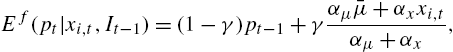
(8) Varf(pt|xi,t,It−1)=γ2Var(μ|xi,t,It−1)=γ2αμ+αx,

where γ∈(0,1]![]() is a constant, measuring the convergence speed of the market price to the expected fundamental value. Note that αμˉμ+αxxi,tαμ+αx
is a constant, measuring the convergence speed of the market price to the expected fundamental value. Note that αμˉμ+αxxi,tαμ+αx![]() and 1αμ+αx
and 1αμ+αx![]() are agent i's posterior updating of the mean and variance, respectively, of the fundamental value of the risky asset conditional on her signal xi,t
are agent i's posterior updating of the mean and variance, respectively, of the fundamental value of the risky asset conditional on her signal xi,t![]() . Condition (7) means that the predicted price is a weighted average of the latest market price and the posterior updating of the fundamental value conditional on her private signal xi,t
. Condition (7) means that the predicted price is a weighted average of the latest market price and the posterior updating of the fundamental value conditional on her private signal xi,t![]() ; while (8) means that the conditional variance is proportional to the posterior variance conditional on the private signal xi,t
; while (8) means that the conditional variance is proportional to the posterior variance conditional on the private signal xi,t![]() . In particular, when γ=1
. In particular, when γ=1![]() , the conditional mean and variance (7)–(8) are reduced to the posterior mean and variance, respectively. Therefore the fundamental trading strategy reflects agent's belief that the future price is expected to converge to the expected fundamental value. Though the private signals xi,t
, the conditional mean and variance (7)–(8) are reduced to the posterior mean and variance, respectively. Therefore the fundamental trading strategy reflects agent's belief that the future price is expected to converge to the expected fundamental value. Though the private signals xi,t![]() are i.i.d. across agents and over time, they are partially incorporated through the current market price pt
are i.i.d. across agents and over time, they are partially incorporated through the current market price pt![]() and hence reflected in the prediction of the future prices. Consequently, the optimal demand based on the fundamental analysis becomes qfi,t=[αμˉμ+αxxi,t−(αμ+αx)pt−1]/(aγ)
and hence reflected in the prediction of the future prices. Consequently, the optimal demand based on the fundamental analysis becomes qfi,t=[αμˉμ+αxxi,t−(αμ+αx)pt−1]/(aγ)![]() , which is called the fundamental trading strategy f.
, which is called the fundamental trading strategy f.
The momentum trading is however independent of the private signal xi,t![]() , but depends on a price trend,
, but depends on a price trend,
(9) Ec(pt|xi,t,It−1)=pt−1+β(pt−1−vt),Varc(pt|xi,t,It−1)=σ2t−1,
where vt![]() is a reference price or price trend (can be a moving average, a supporting/resistance price level, or any index derived from technical analysis), β measures the extrapolation of the price deviation from the trend, and σ2t−1
is a reference price or price trend (can be a moving average, a supporting/resistance price level, or any index derived from technical analysis), β measures the extrapolation of the price deviation from the trend, and σ2t−1![]() is a heuristic prediction on the variance of the asset price. Then the optimal demand becomes qci,t=β(pt−1−vt)/(aσ2t−1)
is a heuristic prediction on the variance of the asset price. Then the optimal demand becomes qci,t=β(pt−1−vt)/(aσ2t−1)![]() , which is called momentum strategy c. In particular, when vt
, which is called momentum strategy c. In particular, when vt![]() is a moving average of the historical prices and β>(<)0
is a moving average of the historical prices and β>(<)0![]() , strategy c is essentially a time-series momentum (contrarian) strategy (Moskowitz et al., 2012).
, strategy c is essentially a time-series momentum (contrarian) strategy (Moskowitz et al., 2012).
Given the information uncertainty, the agent compares the expected value functions based on the two optimal trading strategies and chooses the one with relative higher value. More explicitly, the agent firstly calculates the respective value functions based on strategy f and c,
Efi,t(U)=−exp{−A[Wi,t−1+[αμˉμ+αxxi,t−(αμ+αx)pt−1]22a(αμ+αx)]},Eci,t(U)=−exp{−A[Wi,t−1+β2(pt−1−vt)22aσ2t−1]}.
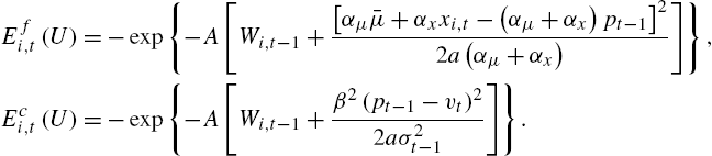
The agent then compares the value functions and selects the one that yields a higher value. Note that Efi,t![]() is an increasing function of the absolute value of the signal |xi,t|
is an increasing function of the absolute value of the signal |xi,t|![]() , while Eci
, while Eci![]() is independent of xi,t
is independent of xi,t![]() . Therefore there exists threshold signal values ˉxt
. Therefore there exists threshold signal values ˉxt![]() for the private signal such that Efi,t=Eci,t
for the private signal such that Efi,t=Eci,t![]() , that is,
, that is,
Efi,t(U)Eci,t(U)=exp{−[[αμˉμ+αxˉxt−(αμ+αx)pt−1]22(αμ+αx)−β2(pt−1−vt)22σ2t−1]}=1.

Solving for ˉxt![]() yields
yields
(10) x±t=1αx[(αμ+αx)pt−1−αμˉμ±β√αμ+αxσt−1(pt−1−vt)].

Therefore, when vt=pt−1![]() , the agent chooses strategy f. When vt≠pt−1
, the agent chooses strategy f. When vt≠pt−1![]() , the agent chooses strategy c if her signal is less informative, falling into the interval (xmt,xMt)
, the agent chooses strategy c if her signal is less informative, falling into the interval (xmt,xMt)![]() , and strategy f otherwise, where xmt=min(x±t)
, and strategy f otherwise, where xmt=min(x±t)![]() and xMt=max(x±t)
and xMt=max(x±t)![]() . Therefore, the optimal demand of agent i is given by qi,t=qfi,t
. Therefore, the optimal demand of agent i is given by qi,t=qfi,t![]() for xi,t⩽xmt
for xi,t⩽xmt![]() or xi,t⩾xMt
or xi,t⩾xMt![]() ; otherwise qi,t=qci,t
; otherwise qi,t=qci,t![]() when xi,t∈(xmt,xMt)
when xi,t∈(xmt,xMt)![]() . Intuitively, when agent's private signal is near the mean fundamental value, the private information becomes less valuable. However, when agent's private signal is far away from the mean fundamental value, the private information becomes more valuable and hence the agent favors the fundamental trading strategy.
. Intuitively, when agent's private signal is near the mean fundamental value, the private information becomes less valuable. However, when agent's private signal is far away from the mean fundamental value, the private information becomes more valuable and hence the agent favors the fundamental trading strategy.
The choice between the two strategies due to the informativeness of the private information about the fundamental value leads to endogenous heterogeneity and switching behavior of agents' choices. More explicitly, by aggregating the demand Dt![]() in a closed form and considering noisy supply St
in a closed form and considering noisy supply St![]() , the market price is determined through a market maker scenario via pt=pt−1+λ(Dt+St)
, the market price is determined through a market maker scenario via pt=pt−1+λ(Dt+St)![]() with λ>0
with λ>0![]() . He and Zheng (2016) first conduct an analysis on the underlying deterministic model when σ2t−1=σ2
. He and Zheng (2016) first conduct an analysis on the underlying deterministic model when σ2t−1=σ2![]() is a constant and vt=pt−2
is a constant and vt=pt−2![]() (corresponding to a simple momentum trading based on the change in the last price). They show that the fundamental price is locally stable with small precisions of the fundamental information noise. That is, the fundamental price becomes unstable when the level of the fundamental information noise is small, leading to high price volatility. Intuitively, in this case, the fundamental information become more accurate and hence less valuable. Therefore the fundamental strategy becomes less profitable, while the momentum trading strategy becomes more popular. This is consistent with the literature on coordination game with imperfect information (see Angeletos and Werning, 2006).
(corresponding to a simple momentum trading based on the change in the last price). They show that the fundamental price is locally stable with small precisions of the fundamental information noise. That is, the fundamental price becomes unstable when the level of the fundamental information noise is small, leading to high price volatility. Intuitively, in this case, the fundamental information become more accurate and hence less valuable. Therefore the fundamental strategy becomes less profitable, while the momentum trading strategy becomes more popular. This is consistent with the literature on coordination game with imperfect information (see Angeletos and Werning, 2006).
When the fundamental price becomes unstable, the price dynamics can become very complicated. On the stochastic model, they have shown that the market fraction of the agents choosing the momentum (fundamental) strategy decreases (increases) as the mis-pricing increases. This underlies mean-reverting of market price to its fundamental price when mis-pricing becomes significant, burst of a bubble, and recover of a recession. This mechanism, together with the destabilizing role of the momentum trading and the stabilizing role of the fundamental trading, provides an endogenous self-correction mechanism of the market. This mechanism is very different from the HAMs with complete information, in which the mean-reverting is channeled through some nonlinear assumptions on the demand or order flow of risky asset. The market stability depends exogenously on balanced activities from fundamental and momentum trading. This integrated approach of HAMs and incomplete information about the fundamental value therefore provides a micro-foundation to endogenous trading heterogeneity and switching behavior wildly characterized in HAMs. Furthermore, He and Zheng (2016) conduct a time series analysis on the stylized facts and demonstrate that the model is able to match the S&P 500 in terms of power-law distribution in returns, volatility clustering, long memory in volatility, and leverage effect.
2.4 Switching of Agents, Fund Flows, and Leverage
Similar to Dieci et al. (2006), most HAMs employ the discrete-choice framework4 to capture the way investors switch across different competing strategies/behavioral rules. However, since this approach models the changes of investors' proportions, not directly the flows of funds, it is not very suitable to capture the long-run performance of investment strategies (or ‘styles’) in terms of accumulated wealth, nor the impact of fund flows on the price dynamics. For this reason, LeBaron (2011) defines such forms of switching between strategies as active learning, capturing investors' tendency to adopt the best-performing rule, in contrast to passive learning, by which investors' wealth naturally accumulates on strategies that have been relatively successful. This second form of learning is closely related to the issue of survival and long-run dominance of strategies and to the evolutionary finance approach (see Blume and Easley, 1992, 2006, Sandroni, 2000, Hens and Schenk-Hoppé, 2005, as well as Evstigneev et al., 2009 for a comprehensive survey of early results and recent research in this field).5
LeBaron (2011) argues that the dynamics of real-world markets are likely to be affected by some combinations of active and passive learning, and that exploring their interaction may improve our understanding of the dynamics of asset prices. Moreover, LeBaron (2012) proposes a simple framework that can simultaneously account for wealth dynamics and active search for new strategies, based on performance comparison. Besides reproducing the basic stylized facts of asset returns and trading volume, the model yields some insight into the dynamics of agents' strategies and their impact on market stability.
A further recent contribution on the interplay of active and passive learning is provided by Palczewski et al. (2016). They build an evolutionary finance framework in discrete time with fundamental, trend-following and noise trading strategies. Such strategies are interpreted as portfolio managers with different investment ‘styles’. Individual investors can move (part of) their funds between portfolio managers. The total amount of freely flowing capital is a model parameter, capturing the clients' degree of impatience (similar to the proportion of switching investors in Dieci et al., 2006). Funds are reallocated based on the relative performance of competing fund managers, according to the discrete choice principle. Therefore, portfolio managers may experience an exogenous growth of their wealth, in addition to the endogenous growth due to returns on the employed capital. The model framework appears promising to investigate the market impact of the fund flows and to incorporate different types of ‘behavioral biases’ into HAMs. In particular, Palczewski et al. (2016) show that even a small amount of freely flowing capital can have a large impact on price movements if investors exhibit ‘recency bias’ in evaluating fund performance.
In a somewhat related framework with heterogeneous investment funds using ‘value investing’, Thurner et al. (2012) explore the joint impact of wealth dynamics and the flows of capital among competing investment funds. Evolutionary pressure generated by short-run competition forces fund managers to make leveraged asset purchases with margin calls. Simulation results highlight a new mechanism to fat tails and clustered volatility, which is linked to wealth dynamics and leverage-induced crashes. Moreover, this framework appears promising to test different credit regulation policies (Poledna et al., 2014) and to investigate the impact of bank leverage management on the stability properties of the financial system (Aymanns and Farmer, 2015).
3 HAMs of Single Asset Market in Continuous-Time
Historical information plays a very important role in testing efficient market hypothesis in financial markets. In particular, it is crucial to understand how quickly market prices reflect fundamental shocks and how much information is contained in the historical prices. Empirical evidence shows that stock markets react with a delay to information on fundamentals and that information diffuses gradually across markets (Hou and Moskowitz, 2005, Hong et al., 2007). Based on market underreaction and overreaction hypotheses, momentum and contrarian strategies are widely used by financial market practitioners and their profitability has been extensively investigated by academics. De Bondt and Thaler (1985) and Lakonishok et al. (1994) find supporting evidence on the profitability of contrarian strategies for a holding period of 3–5 years based on the past 3–5 years' returns. In contrast, Jegadeesh and Titman (1993, 2001) among many others, find supporting evidence on the profitability of momentum strategies for holding periods of 3–12 months based on the returns over the past 3–12 months. Time series momentum investigated recently in Moskowitz et al. (2012) characterizes a strong positive predictability of a security's own past returns. It becomes clear that the time horizons of historical prices play crucial roles in the performance of contrarian and momentum strategies. Many theoretical studies have tried to explain the momentum,6 however, as argued in Griffin et al. (2003), “the comparison is in some sense unfair since no time horizon is specified in most behavioral models”.
In the literature of HAMs, the heterogeneous expectations of agents, in particular of chartists, are formed based on price trends such as moving average of historical prices. In discrete-time models, with different time horizon, the dimension of the model is different. To examine the effect of time horizon analytically, we need to study the model with different dimension separately. Also, as the time horizon increases, it becomes more difficult analytically in dealing with high dimensional nonlinear dynamic system. This challenge is illustrated in Chiarella et al. (2006b) when examining the effect of different moving averages on market stability. Therefore, how different time horizons of historical prices affect price dynamics becomes a challenging issue in the current HAMs.
This section introduces some of the recent developments of HAMs of a single risky asset (and a riskless asset) in continuous time to deal with the price delay problems in behavioral finance and HAMs literature. In continuous-time HAMs, the time horizon of historical price information is simply captured by a time delay parameter. Such models are characterized mathematically by a system of stochastic delay differential equations, which provide a more broad framework to investigate the joint effect of adaptive behavior of heterogeneous agents and the impact of historical prices.
Development of deterministic delay differential equation models to characterize fluctuation of commodity prices and cyclic economic behavior has a long history,7 however the application to asset pricing and financial markets is relatively new. This section bridges HAMs with traditional approaches in continuous-time finance to investigate the impact of moving average rules over different time horizon (He and Li, 2012) in Section 3.1, the profitability of fundamental and momentum strategies (He and Li, 2015a) in Section 3.2, and optimal asset allocation with time series momentum and reversal (He et al., 2018) in Section 3.3.
3.1 A Continuous-Time HAM with Time Delay
We now introduce the continuous-time model of He and Li (2012) and demonstrate first that the result of Brock and Hommes on rational routes to market instability in discrete-time also holds in continuous time. That is, adaptive switching behavior of agents can lead to market instability as the switching intensity increases. We then show a double edged effect of an increase in the time horizon of historical price information on market stability. An initial increase in time delay can destabilize the market, leading to price fluctuations. However, as the time delay increases further, the market is stabilized. This double edged effect is a very different feature of continuous-time HAMs from discrete-time HAMs. With noisy fundamental value and liquidity traders, the continuous-time model is able to generate long deviations of market price from the fundamental price, bubbles, crashes, and volatility clustering.
Consider a financial market with a risky asset and let P(t)![]() denote the (cum) price per share of the risky asset at time t. The market consists of fundamentalists, chartists, liquidity traders, and a market maker. The fundamentalists believe that the market price P(t)
denote the (cum) price per share of the risky asset at time t. The market consists of fundamentalists, chartists, liquidity traders, and a market maker. The fundamentalists believe that the market price P(t)![]() is mean-reverting to the fundamental price F(t)
is mean-reverting to the fundamental price F(t)![]() , and their demand is given by Zf(t)=βf[F(t)−P(t)]
, and their demand is given by Zf(t)=βf[F(t)−P(t)]![]() , with βf>0
, with βf>0![]() measuring the mean-reverting speed of the market price to the fundamental price. The chartists are modeled as trend followers, believing that the future market price follows a price trend u(t)
measuring the mean-reverting speed of the market price to the fundamental price. The chartists are modeled as trend followers, believing that the future market price follows a price trend u(t)![]() , and their demand is given by8 Zc(t)=tanh(βc[P(t)−u(t)])
, and their demand is given by8 Zc(t)=tanh(βc[P(t)−u(t)])![]() with βc>0
with βc>0![]() measuring the extrapolation of the trend followers to the price trend. Among various price trends used in practice, we consider u(t)
measuring the extrapolation of the trend followers to the price trend. Among various price trends used in practice, we consider u(t)![]() as a normalized exponentially decaying weighted average of historical prices over a time interval [t−τ,t]
as a normalized exponentially decaying weighted average of historical prices over a time interval [t−τ,t]![]() ,
,
(11) u(t)=k1−e−kτ∫tt−τe−k(t−s)P(s)ds,

where time delay τ∈(0,∞)![]() represents time horizon of historical prices, k>0
represents time horizon of historical prices, k>0![]() measures the decay rate of the weights on the historical prices. In particular, when k→0
measures the decay rate of the weights on the historical prices. In particular, when k→0![]() , the weights are equal and the price trend u(t)
, the weights are equal and the price trend u(t)![]() in (11) is simply given by the standard moving average (MA) with equal weights, u(t)=1τ∫tt−τP(s)ds
in (11) is simply given by the standard moving average (MA) with equal weights, u(t)=1τ∫tt−τP(s)ds![]() . When k→∞
. When k→∞![]() , all the weights go to the current price so that u(t)→P(t)
, all the weights go to the current price so that u(t)→P(t)![]() . For the time delay, when τ→0
. For the time delay, when τ→0![]() , the trend followers regard the current price as the price trend. When τ→∞
, the trend followers regard the current price as the price trend. When τ→∞![]() , the trend followers use all the historical prices to form the price trend, u(t)=k∫t−∞e−k(t−s)P(s)ds
, the trend followers use all the historical prices to form the price trend, u(t)=k∫t−∞e−k(t−s)P(s)ds![]() . In general, for 0<k<∞
. In general, for 0<k<∞![]() , Eq. (11) can be expressed as a delay differential equation with time delay τ
, Eq. (11) can be expressed as a delay differential equation with time delay τ
du(t)=k1−e−kτ[P(t)−e−kτP(t−τ)−(1−e−kτ)u(t)]dt.
The demand of liquidity traders is i.i.d. normally distributed with mean of zero and standard deviation of σM(>0)![]() .
.
Let nf(t)![]() and nc(t)
and nc(t)![]() represent the market fractions of agents who use the fundamental and trend following strategies, respectively. Their net profits over a short time interval [t,t+dt]
represent the market fractions of agents who use the fundamental and trend following strategies, respectively. Their net profits over a short time interval [t,t+dt]![]() can be measured, respectively, by πf(t)dt=Zf(t)dP(t)−Cfdt
can be measured, respectively, by πf(t)dt=Zf(t)dP(t)−Cfdt![]() and πc(t)dt=Zc(t)dP(t)−Ccdt
and πc(t)dt=Zc(t)dP(t)−Ccdt![]() , where Cf,Cc⩾0
, where Cf,Cc⩾0![]() are constant costs of the strategies. To measure strategy performance, we introduce a cumulated profit over the time interval [t−τ,t]
are constant costs of the strategies. To measure strategy performance, we introduce a cumulated profit over the time interval [t−τ,t]![]() by Ui(t)=η1−e−ητ∫tt−τe−η(t−s)πi(s)ds,i=f,c
by Ui(t)=η1−e−ητ∫tt−τe−η(t−s)πi(s)ds,i=f,c![]() , where η>0
, where η>0![]() measures the decay of the historical profits. Consequently, dUi(t)=η[πi(t)−e−ητπi(t−τ)1−e−ητ−Ui(t)]dt
measures the decay of the historical profits. Consequently, dUi(t)=η[πi(t)−e−ητπi(t−τ)1−e−ητ−Ui(t)]dt![]() for i=f,c
for i=f,c![]() . Following Hofbauer and Sigmund (1998, Chapter 7), the evolution dynamics of the market populations are governed by
. Following Hofbauer and Sigmund (1998, Chapter 7), the evolution dynamics of the market populations are governed by
dni(t)=βni(t)[dUi(t)−dˉU(t)], for i=f,c,
where dˉU(t)=nf(t)dUf(t)+nc(t)dUc(t)![]() is the average performance of the two strategies and β>0
is the average performance of the two strategies and β>0![]() measures the intensity of choice. The switching mechanism in the continuous-time setup is consistent with the one used in discrete-time HAMs. In fact, it can be verified that the dynamics of the market fraction nf(t)
measures the intensity of choice. The switching mechanism in the continuous-time setup is consistent with the one used in discrete-time HAMs. In fact, it can be verified that the dynamics of the market fraction nf(t)![]() satisfy dnf(t)=βnf(t)(1−nf(t))[dUf(t)−dUc(t)]
satisfy dnf(t)=βnf(t)(1−nf(t))[dUf(t)−dUc(t)]![]() , leading to nf(t)=eβUf(t)/(eβUf(t)+eβUc(t))
, leading to nf(t)=eβUf(t)/(eβUf(t)+eβUc(t))![]() , which is the discrete choice model used in Brock and Hommes (1998).
, which is the discrete choice model used in Brock and Hommes (1998).
Finally, the price P(t)![]() is adjusted by the market maker according to dP(t)=μ[nf(t)Zf(t)+nc(t)Zc(t)]dt+σMdWM(t)
is adjusted by the market maker according to dP(t)=μ[nf(t)Zf(t)+nc(t)Zc(t)]dt+σMdWM(t)![]() , where μ>0
, where μ>0![]() represents the speed of the price adjustment of the market maker, WM(t)
represents the speed of the price adjustment of the market maker, WM(t)![]() is a standard Wiener process capturing the random excess demand process either driven by unexpected market news or liquidity traders, and σM>0
is a standard Wiener process capturing the random excess demand process either driven by unexpected market news or liquidity traders, and σM>0![]() is a constant. To sum up, the market price of the risky asset is determined according to the stochastic delay differential system
is a constant. To sum up, the market price of the risky asset is determined according to the stochastic delay differential system
(12) {dP(t)=μ[nf(t)Zf(t)+(1−nf(t))Zc(t)]dt+σMdWM(t),du(t)=k1−e−kτ[P(t)−e−kτP(t−τ)−(1−e−kτ)u(t)]dt,dU(t)=η1−e−ητ[π(t)−e−ητπ(t−τ)−(1−e−ητ)U(t)]dt,
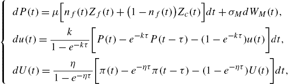
where U(t)=Uf(t)−Uc(t)![]() , nf(t)=1/(1+e−βU(t))
, nf(t)=1/(1+e−βU(t))![]() , Zf(t)=βf(F(t)−P(t))
, Zf(t)=βf(F(t)−P(t))![]() , Zc(t)=tanh[βc(P(t)−u(t))]
, Zc(t)=tanh[βc(P(t)−u(t))]![]() , C=Cf−Cc
, C=Cf−Cc![]() , and
, and
π(t)=πf(t)−πc(t)=μ[nf(t)Zf(t)+(1−nf(t))Zc(t)][Zf(t)−Zc(t)]−C.
By assuming that the fundamental price is a constant F(t)≡ˉF![]() and there is no market noise σM=0
and there is no market noise σM=0![]() , system (12) becomes a deterministic delay differential system with (P,u,U)=(ˉF,ˉF,−C)
, system (12) becomes a deterministic delay differential system with (P,u,U)=(ˉF,ˉF,−C)![]() as the unique fundamental steady state. He and Li (2012) show that the steady state is locally stable for either small or large time delay τ when the market is dominated by the fundamentalists. Otherwise, the steady state becomes unstable through Hopf bifurcations as the time delay increases. This result is in line with the results obtained in discrete-time HAMs. However, different from discrete-time HAMs, the continuous-time model shows that the fundamental steady state becomes locally stable again when the time delay is large enough. This is illustrated by the bifurcation diagram of the market price with respect to τ in Fig. 4A.9 It shows that there are two Hopf bifurcation values 0<τo<τ1
as the unique fundamental steady state. He and Li (2012) show that the steady state is locally stable for either small or large time delay τ when the market is dominated by the fundamentalists. Otherwise, the steady state becomes unstable through Hopf bifurcations as the time delay increases. This result is in line with the results obtained in discrete-time HAMs. However, different from discrete-time HAMs, the continuous-time model shows that the fundamental steady state becomes locally stable again when the time delay is large enough. This is illustrated by the bifurcation diagram of the market price with respect to τ in Fig. 4A.9 It shows that there are two Hopf bifurcation values 0<τo<τ1![]() occurring at τ=τ0(≈8)
occurring at τ=τ0(≈8)![]() and τ=τ1(≈28)
and τ=τ1(≈28)![]() . The fundamental steady state is locally stable when the time delay is small, τ∈[0,τ0)
. The fundamental steady state is locally stable when the time delay is small, τ∈[0,τ0)![]() , then becomes unstable for τ∈(τo,τ1)
, then becomes unstable for τ∈(τo,τ1)![]() , and then regains the local stability for τ>τ1
, and then regains the local stability for τ>τ1![]() . Due to the problem of high dimensionality, such analysis on the effect of historical price on market price in discrete-time HAMs can become very complicated, see Chiarella et al. (2006b) that examining the effect of different moving averages on market stability. It is the continuous-time model that facilitates such analysis on the stability effect of time horizon of historical prices and stability switching. The bifurcation diagram of the market price with respect to the switching intensity β is given in Fig. 4B. It shows that the fundamental steady state is locally stable when the switching intensity β is low, becoming unstable as the switching intensity increases, bifurcating to periodic price with increasing fluctuations. This is consistent with the discrete-time HAMs.
. Due to the problem of high dimensionality, such analysis on the effect of historical price on market price in discrete-time HAMs can become very complicated, see Chiarella et al. (2006b) that examining the effect of different moving averages on market stability. It is the continuous-time model that facilitates such analysis on the stability effect of time horizon of historical prices and stability switching. The bifurcation diagram of the market price with respect to the switching intensity β is given in Fig. 4B. It shows that the fundamental steady state is locally stable when the switching intensity β is low, becoming unstable as the switching intensity increases, bifurcating to periodic price with increasing fluctuations. This is consistent with the discrete-time HAMs.
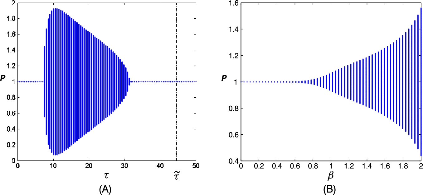
For the deterministic model, when the steady state becomes unstable, it bifurcates to stable periodic solutions through a Hopf bifurcation. The periodic fluctuations of the market prices are associated with periodic fluctuations of the market fractions, illustrated in Fig. 5A. Based on the bifurcation diagram in Fig. 4A, the steady state is unstable for τ=16![]() . Fig. 5A shows that both price and market fraction fluctuate periodically. It shows that, when the fundamental steady state becomes unstable, the market fractions tend to stay away from the steady state market fraction level most of the time and a mean of nf
. Fig. 5A shows that both price and market fraction fluctuate periodically. It shows that, when the fundamental steady state becomes unstable, the market fractions tend to stay away from the steady state market fraction level most of the time and a mean of nf![]() below 0.5 clearly indicates the dominance of the trend following strategy. To examine the effect of population evolution, we compare the case without switching β=0
below 0.5 clearly indicates the dominance of the trend following strategy. To examine the effect of population evolution, we compare the case without switching β=0![]() to the case with switching β≠0
to the case with switching β≠0![]() . Fig. 5A clearly shows that the evolution of population increases the fluctuations in both price and market fraction.
. Fig. 5A clearly shows that the evolution of population increases the fluctuations in both price and market fraction.

For the stochastic model with a random walk fundamental price process, Fig. 5B demonstrates that the market price follows the fundamental price closely when τ=3![]() , while Fig. 5C illustrates that the market price fluctuates around the fundamental price in cyclical fashion for τ=16
, while Fig. 5C illustrates that the market price fluctuates around the fundamental price in cyclical fashion for τ=16![]() . To examine the effect of population evolution, we compare the case without switching β=0
. To examine the effect of population evolution, we compare the case without switching β=0![]() to the case with switching β≠0
to the case with switching β≠0![]() . Fig. 5B shows that the evolution of population has insignificant impact on the price dynamics when the fundamental steady state of the underlying deterministic model is locally stable for τ=3
. Fig. 5B shows that the evolution of population has insignificant impact on the price dynamics when the fundamental steady state of the underlying deterministic model is locally stable for τ=3![]() . However, when the fundamental steady state becomes unstable for τ=16
. However, when the fundamental steady state becomes unstable for τ=16![]() , the fluctuations in both price and market fraction become more significant. Therefore the stochastic price behavior is underlined by the dynamics of the corresponding deterministic model. He and Li (2012) further explore the potential of the stochastic model in generating volatility clustering and long range dependence in volatility. The underlying mechanism and the interplay between the nonlinear deterministic dynamics and noises are very similar to the discrete-time HAM by He and Li (2007). The framework can be used to study the joint impact of many heterogeneous strategies based on different time horizons of historical prices on market stability.
, the fluctuations in both price and market fraction become more significant. Therefore the stochastic price behavior is underlined by the dynamics of the corresponding deterministic model. He and Li (2012) further explore the potential of the stochastic model in generating volatility clustering and long range dependence in volatility. The underlying mechanism and the interplay between the nonlinear deterministic dynamics and noises are very similar to the discrete-time HAM by He and Li (2007). The framework can be used to study the joint impact of many heterogeneous strategies based on different time horizons of historical prices on market stability.
3.2 Profitability of Momentum and Contrarian Strategies
Momentum and contrarian strategies are widely used by market practitioners to profit from momentum in the short-run and mean-reversion in the long-run in financial markets. Empirical profitability of these strategies based on moving averages with different time horizon of historical prices and different holding period has been extensively investigated in the literature (Lakonishok et al., 1994, Jegadeesh and Titman, 1993, 2001, and Moskowitz et al., 2012).
To explain the profitability and the underlying mechanism of time series momentum and contrarian strategies, He and Li (2015a) propose a continuous-time HAM consisting of fundamental, momentum, and contrarian traders. They develop an intuitive and parsimonious financial market model of heterogeneous agents to study the impact of different time horizons on market price and profitability of fundamental, momentum and contrarian trading strategies. They show that the performance of momentum strategy is determined by the historical time horizon, investment holding period, and market dominance of momentum trading. More specifically, due to price continuity, the price trend based on the moving average of historical prices becomes very significant (apart from over very short time horizon). Therefore, when momentum traders are more active in the market, the price trend becomes very sensitive to the shocks, which is characterized by the destabilizing role of the momentum trading to the market. This provides a profit opportunity for momentum trading with short, not long, holding time horizons. When momentum traders are less active in the market, they always loose. The results provide some insights into the profitability of time series momentum over short, not long, holding periods. We now brief the main results of He and Li (2015a).
Consider a continuous-time model with fundamentalists who trade according to fundamental analysis and momentum and contrarian traders who trade differently based on price trend calculated from moving averages of historical prices over different time horizons. Let P(t)![]() and F(t)
and F(t)![]() denote the log (cum dividend) price and (log) fundamental value10 of a risky asset at time t, respectively. The fundamental traders buy (sell) the stock when the current price P(t)
denote the log (cum dividend) price and (log) fundamental value10 of a risky asset at time t, respectively. The fundamental traders buy (sell) the stock when the current price P(t)![]() is below (above) the fundamental value F(t)
is below (above) the fundamental value F(t)![]() . For simplicity, we assume that the fundamental return follows a pure white noise process dF(t)=σFdWF(t)
. For simplicity, we assume that the fundamental return follows a pure white noise process dF(t)=σFdWF(t)![]() with F(0)=ˉF
with F(0)=ˉF![]() , σF>0
, σF>0![]() , and WF(t)
, and WF(t)![]() is a standard Wiener process.
is a standard Wiener process.
Regarding the momentum and contrarian trading, as in the previous section, we assume that both momentum and contrarian traders trade based on their estimated market price trends, although they behave differently. Momentum traders believe that future market price follows a price trend um(t)![]() , while contrarians believe that future market price goes opposite to a price trend uc(t)
, while contrarians believe that future market price goes opposite to a price trend uc(t)![]() . The price trend used for the momentum traders and contrarians can be different in general. Among various price trends used in practice, the standard moving average (MA) rules with different time horizons are the most popular ones, ui(t)=1τi∫tt−τiP(s)ds
. The price trend used for the momentum traders and contrarians can be different in general. Among various price trends used in practice, the standard moving average (MA) rules with different time horizons are the most popular ones, ui(t)=1τi∫tt−τiP(s)ds![]() for i=m,c
for i=m,c![]() , where the time delay τi≥0
, where the time delay τi≥0![]() represents the time horizon of the MA. Assume the excess demand of the momentum traders and contrarians are given, respectively, by Zm(t)=gm(P(t)−um(t))
represents the time horizon of the MA. Assume the excess demand of the momentum traders and contrarians are given, respectively, by Zm(t)=gm(P(t)−um(t))![]() and Dc(t)=gc(uc(t)−P(t))
and Dc(t)=gc(uc(t)−P(t))![]() , where gi(x)
, where gi(x)![]() satisfies gi(0)=0,g′i(x)>0,g′i(0)=βi>0,xg″i(x)<0
satisfies gi(0)=0,g′i(x)>0,g′i(0)=βi>0,xg″i(x)<0![]() for x≠0
for x≠0![]() and i=m,c
and i=m,c![]() , and parameter βi
, and parameter βi![]() represents the extrapolation rate when the market price deviation from the trend is small.
represents the extrapolation rate when the market price deviation from the trend is small.
Assume a zero net supply in the risky asset and let αf![]() , αm
, αm![]() , and αc
, and αc![]() be the fixed market population fractions of the fundamental, momentum, and contrarian traders,11 respectively, with αf+αm+αc=1
be the fixed market population fractions of the fundamental, momentum, and contrarian traders,11 respectively, with αf+αm+αc=1![]() . Following Beja and Goldman (1980) and Farmer and Joshi (2002), the price P(t)
. Following Beja and Goldman (1980) and Farmer and Joshi (2002), the price P(t)![]() at time t is determined by
at time t is determined by
(13) dP(t)=μ[αfZf(t)+αmZm(t)+αcZc(t)]dt+σMdWM(t),
where μ>0![]() represents the speed of the price adjustment of the market maker, WM(t)
represents the speed of the price adjustment of the market maker, WM(t)![]() is a standard Wiener process, independent of WF(t)
is a standard Wiener process, independent of WF(t)![]() , capturing the random demand of either noise or liquidity traders, and σM≥0
, capturing the random demand of either noise or liquidity traders, and σM≥0![]() is constant.
is constant.
By assuming a constant fundamental price F(t)≡ˉF![]() and no market noise σM=0
and no market noise σM=0![]() , system (13) becomes a deterministic delay integro-differential equation,
, system (13) becomes a deterministic delay integro-differential equation,
(14) dP(t)dt=μ[αfβf(ˉF−P(t))+αmtanh(βm(P(t)−1τm∫tt−τmP(s)ds))+αctanh(−βc(P(t)−1τc∫tt−τcP(s)ds))].
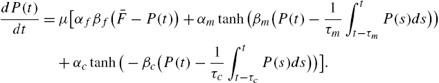
It is easy to see that P(t)=ˉF![]() , the fundamental steady state, is the unique steady state price of system (14). He and Li (2015a) examine different role of the time horizon used in the MA by either the contrarians or momentum traders. When both strategies are employed in the market, the market stability of system (14) can be characterized by the following proposition.
, the fundamental steady state, is the unique steady state price of system (14). He and Li (2015a) examine different role of the time horizon used in the MA by either the contrarians or momentum traders. When both strategies are employed in the market, the market stability of system (14) can be characterized by the following proposition.
Proposition 3.1
If τm=τc=τ![]() , then the fundamental steady state price P=ˉF
, then the fundamental steady state price P=ˉF![]() of system (14) is
of system (14) is
- 1. locally stable for all τ⩾0
 when γm<γc+γf/(1+a)
 ;
; - 2. locally stable for either 0⩽τ<τ⁎l
 or τ>τ⁎h
 and unstable for τ⁎l<τ<τ⁎h
 when γc+γf/(1+a)≤γm≤γc+γf
 ; and
; and - 3. locally stable for τ<τ⁎l
 and unstable for τ>τ⁎l
 when γm>γc+γf
 .
.
Here τ⁎1=2(γm−γc)/(γf−γm+γc)2![]() , and τ⁎l(<τ⁎1)
, and τ⁎l(<τ⁎1)![]() and τ⁎h(∈(τ⁎l,τ⁎1))
and τ⁎h(∈(τ⁎l,τ⁎1))![]() are the minimum and maximum positive roots, respectively, of the equation
are the minimum and maximum positive roots, respectively, of the equation
τγm−γc(γf−γm+γc)2−cos[√2(γm−γc)τ−(γf−γm+γc)2τ2]−1=0.

The three conditions (1) γm<γc+γf1+a![]() , (2) γc+γf1+a≤γm≤γc+γf
, (2) γc+γf1+a≤γm≤γc+γf![]() , and (3) γm>γc+γf
, and (3) γm>γc+γf![]() in Proposition 3.1 characterize three different states of market stability, having different implications to the profitability of momentum trading. For convenience, market state k is referred to condition (k) for k=1,2,3
in Proposition 3.1 characterize three different states of market stability, having different implications to the profitability of momentum trading. For convenience, market state k is referred to condition (k) for k=1,2,3![]() in the following discussion. Numerical analysis shows that for market state 1, the fundamental price is locally stable, independent of the time horizon; for market state 2, the fundamental price is locally stable when τ∈[0,τ⁎l)∪(τ⁎h,∞)
in the following discussion. Numerical analysis shows that for market state 1, the fundamental price is locally stable, independent of the time horizon; for market state 2, the fundamental price is locally stable when τ∈[0,τ⁎l)∪(τ⁎h,∞)![]() and becomes unstable when τ∈(τ⁎l,τ⁎h)
and becomes unstable when τ∈(τ⁎l,τ⁎h)![]() (the stability switches twice); while for market state 3, the first (Hopf bifurcation) value τ⁎l(≈0.22)
(the stability switches twice); while for market state 3, the first (Hopf bifurcation) value τ⁎l(≈0.22)![]() leads to stable limit cycles for τ>τ⁎l
leads to stable limit cycles for τ>τ⁎l![]() (the stability switches only once at τ⁎l
(the stability switches only once at τ⁎l![]() ).
).
The profitability of different strategies based on the stochastic model is closely related to the market states and holding period. In market state 1, the market is dominated jointly by the fundamental and contrarian traders (so that γm<γc+γf/(1+a)![]() ). In this case, the stability of the fundamental price of the underlying deterministic model is independent of the time horizon. Monte Carlo simulations show that the contrarian and fundamental strategies are profitable, but not the momentum strategy and the market maker, underlined by significant and negative ACs for small lags and insignificant ACs for large lags. This corresponds to market overreaction in short-run and hence the fundamental and contrarian trading can generate significant profits. Without under-reaction in this case, the momentum trading is not profitable.
). In this case, the stability of the fundamental price of the underlying deterministic model is independent of the time horizon. Monte Carlo simulations show that the contrarian and fundamental strategies are profitable, but not the momentum strategy and the market maker, underlined by significant and negative ACs for small lags and insignificant ACs for large lags. This corresponds to market overreaction in short-run and hence the fundamental and contrarian trading can generate significant profits. Without under-reaction in this case, the momentum trading is not profitable.
In market state 2, the momentum traders are active, but their activities are balanced by the fundamental and contrarian traders. In this case, the fundamental and contrarian trading strategies are still profitable, but not the momentum traders and the market maker. This is illustrated by the average accumulated profits based on a typical simulation with time horizon τ=0.5![]() and holding period h=2
and holding period h=2![]() in Fig. 6A. The return ACs based on Monte Carlo simulation show some significantly negative ACs over short lags, indicating the profitability of the fundamental and contrarian trading due to market overreaction, but not for the momentum trading.
in Fig. 6A. The return ACs based on Monte Carlo simulation show some significantly negative ACs over short lags, indicating the profitability of the fundamental and contrarian trading due to market overreaction, but not for the momentum trading.
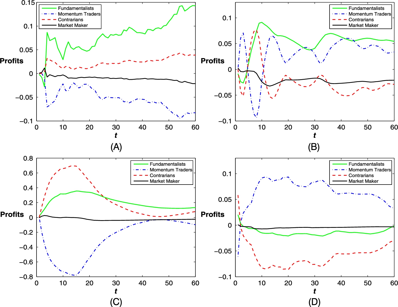
In market state 3, the market is dominated by the momentum traders and their destabilizing role. Over short time horizon, the market price fluctuates due to the unstable fundamental price of the underlying deterministic system. When the market price increases, the price trend follows the market price closely and increases too. The momentum trading with short holding period hence becomes profitable by taking long positions. Similarly, when the market price declines, the price trend follows and hence the momentum trading with short holding period is profitable by taking short positions. Therefore, the momentum trading strategies are profitable, but not the contrarians, illustrated by Fig. 6B for τ=h=0.5![]() and Fig. 6C for τ=h=3
and Fig. 6C for τ=h=3![]() respectively. Over long time horizon, the market price fluctuates widely due to the unstable fundamental value of the underlying deterministic system. A longer time horizon makes the price trend less sensitive to the changes in price and the shocks. The dominance of the momentum trading and market price continuation make the momentum trading with short holding period more profitable, illustrated by Fig. 6D for τ=3
respectively. Over long time horizon, the market price fluctuates widely due to the unstable fundamental value of the underlying deterministic system. A longer time horizon makes the price trend less sensitive to the changes in price and the shocks. The dominance of the momentum trading and market price continuation make the momentum trading with short holding period more profitable, illustrated by Fig. 6D for τ=3![]() and h=0.5
and h=0.5![]() . With long holding period, the momentum trading mis-matches the profitability opportunity and hence becomes less profitable. With long time horizon and long holding period, Fig. 6C also illustrates that the fundamental and contrarian strategies are profitable, but not the momentum strategy. For time horizon and holding period from 1 to 60 months, the model is able to replicate the time series momentum profit explored for the S&P 500. The results are consistent with Moskowitz et al. (2012) who find that the time series momentum strategy with 12 months horizon and one month holding is the most profitable among others.
. With long holding period, the momentum trading mis-matches the profitability opportunity and hence becomes less profitable. With long time horizon and long holding period, Fig. 6C also illustrates that the fundamental and contrarian strategies are profitable, but not the momentum strategy. For time horizon and holding period from 1 to 60 months, the model is able to replicate the time series momentum profit explored for the S&P 500. The results are consistent with Moskowitz et al. (2012) who find that the time series momentum strategy with 12 months horizon and one month holding is the most profitable among others.
In summary, the stochastic delay integro-differential system of the model provides a unified approach to deal with different time horizons of momentum and contrarian strategies. The profitability is closely related to the market states defined by the stability of the underlying deterministic model. In particular, in market state 3 where the momentum traders dominate the market, the momentum strategy is profitable with short, but not long, holding periods. Some explanations to the mechanism of the profitability through autocorrelation patterns and the under-reaction and overreaction hypotheses are also provided in He and Li (2015a).
3.3 Optimal Trading with Time Series Momentum and Reversal
Short-run momentum and long-run reversal are two of the most prominent financial market anomalies. Though market timing opportunities under mean reversion in equity return are well documented (Campbell and Viceira, 1999 and Wachter, 2002), time series momentum (TSM) has been explored recently in Moskowitz et al. (2012). Intuitively, if we incorporate both return momentum and reversal into a trading strategy optimally, we would expect to outperform the strategies based only on return momentum or reversal, and even the market index. To capture this intuition, He et al. (2018) develop a continuous-time asset price model, derive an optimal investment strategy theoretically, and test the strategy empirically. They show that, by combining market fundamentals and timing opportunity with respect to market trend and volatility, the optimal strategy based on the time series momentum and reversal significantly outperforms, both in-sample and out-of-sample, the S&P 500 and pure strategies based on either time series momentum or reversal only. We now outline the main results and refer the details to He et al. (2018).
Consider a financial market with two tradable securities. A riskless asset B satisfies dBt/Bt=rdt![]() with a constant risk-free rate r. The risky asset St
with a constant risk-free rate r. The risky asset St![]() satisfies
satisfies
dSt/St=[ϕmt+(1−ϕ)μt]dt+σ′SdZt,dμt=α(ˉμ−μt)dt+σ′μdZt,
where α>0,ˉμ>0![]() , and mt=(1/τ)∫tt−τdSuSu
, and mt=(1/τ)∫tt−τdSuSu![]() . Here ϕ is a constant, ˉμ
. Here ϕ is a constant, ˉμ![]() is the constant long-run expected return, α measures the speed of the convergence of μt
is the constant long-run expected return, α measures the speed of the convergence of μt![]() to ˉμ
to ˉμ![]() , σS
, σS![]() and σ′μ
and σ′μ![]() are two-dimensional volatility vectors, and Zt
are two-dimensional volatility vectors, and Zt![]() is a two-dimensional vector of independent Brownian motions. Therefore, the expected return is given by a combination of a momentum component mt
is a two-dimensional vector of independent Brownian motions. Therefore, the expected return is given by a combination of a momentum component mt![]() based on a moving average of the past returns and a long-run mean-reversion component μt
based on a moving average of the past returns and a long-run mean-reversion component μt![]() based on market fundamentals such as dividend yield.
based on market fundamentals such as dividend yield.
Consider a typical long-term investor who maximizes the expected log utility of terminal wealth at time T(>t)![]() . Let Wt
. Let Wt![]() be the wealth of the investor at time t and πt
be the wealth of the investor at time t and πt![]() be the fraction of the wealth invested in the stock. Then
be the fraction of the wealth invested in the stock. Then
(15) dWtWt=(πt[ϕmt+(1−ϕ)μt−r]+r)dt+πtσ′SdZt.

By applying the maximum principle for optimal control of stochastic delay differential equations, He et al. (2018) derive the optimal investment strategy
(16) π⁎t=ϕmt+(1−ϕ)μt−rσ′SσS.

That is, by taking into account the short-run momentum and long-run reversal, as well as the timing opportunity with respect to market trend and volatility, a weighted average of the momentum and mean-reverting strategies is optimal.
This result has a number of implications. (i) When the asset price follows a geometric Brownian motion process with mean-reversion drift μt![]() , namely ϕ=0
, namely ϕ=0![]() , the optimal investment strategy (16) becomes π⁎t=μt−rσ′SσS
, the optimal investment strategy (16) becomes π⁎t=μt−rσ′SσS![]() . This is the optimal investment strategy with mean-reverting returns obtained in the literature (Campbell and Viceira, 1999 and Wachter, 2002). In particular, when μt=ˉμ
. This is the optimal investment strategy with mean-reverting returns obtained in the literature (Campbell and Viceira, 1999 and Wachter, 2002). In particular, when μt=ˉμ![]() is a constant, the optimal portfolio collapses to the optimal portfolio of Merton (1971). (ii) When the asset return depends only on the momentum, namely ϕ=1
is a constant, the optimal portfolio collapses to the optimal portfolio of Merton (1971). (ii) When the asset return depends only on the momentum, namely ϕ=1![]() , the optimal portfolio (16) reduces to π⁎t=mt−rσ′SσS
, the optimal portfolio (16) reduces to π⁎t=mt−rσ′SσS![]() . If we consider a trading strategy based on the trading signal indicated by the excess moving average return mt−r
. If we consider a trading strategy based on the trading signal indicated by the excess moving average return mt−r![]() only, with τ=12
only, with τ=12![]() months, the strategy of long/short when the trading signal is positive/negative is consistent with the TSM strategy used in Moskowitz et al. (2012). Therefore, if we only take fixed long/short positions and construct simple buy-and-hold momentum strategies over a large range of look-back and holding periods, the TSM strategy of Moskowitz et al. (2012) can be optimal when the mean reversion is not significant in financial markets.
months, the strategy of long/short when the trading signal is positive/negative is consistent with the TSM strategy used in Moskowitz et al. (2012). Therefore, if we only take fixed long/short positions and construct simple buy-and-hold momentum strategies over a large range of look-back and holding periods, the TSM strategy of Moskowitz et al. (2012) can be optimal when the mean reversion is not significant in financial markets.
He et al. (2018) then examine the performance of the optimal portfolio in terms of the utility of the portfolio wealth empirically. As a benchmark, the log utility of $1 investment in the S&P 500 index from January 1876 grows to 5.765 at December 2012. With a time horizon of τ=12![]() and one month holding period, the optimal portfolio wealth fractions and the evolution of the utility of the optimal portfolio wealth (lnW⁎t
and one month holding period, the optimal portfolio wealth fractions and the evolution of the utility of the optimal portfolio wealth (lnW⁎t![]() ) based on the estimated model from January 1876 to December 2012 are plotted in Fig. 7A and B, showing that the optimal portfolios outperform the market index measured by the utility of wealth (lnWt
) based on the estimated model from January 1876 to December 2012 are plotted in Fig. 7A and B, showing that the optimal portfolios outperform the market index measured by the utility of wealth (lnWt![]() ).
).
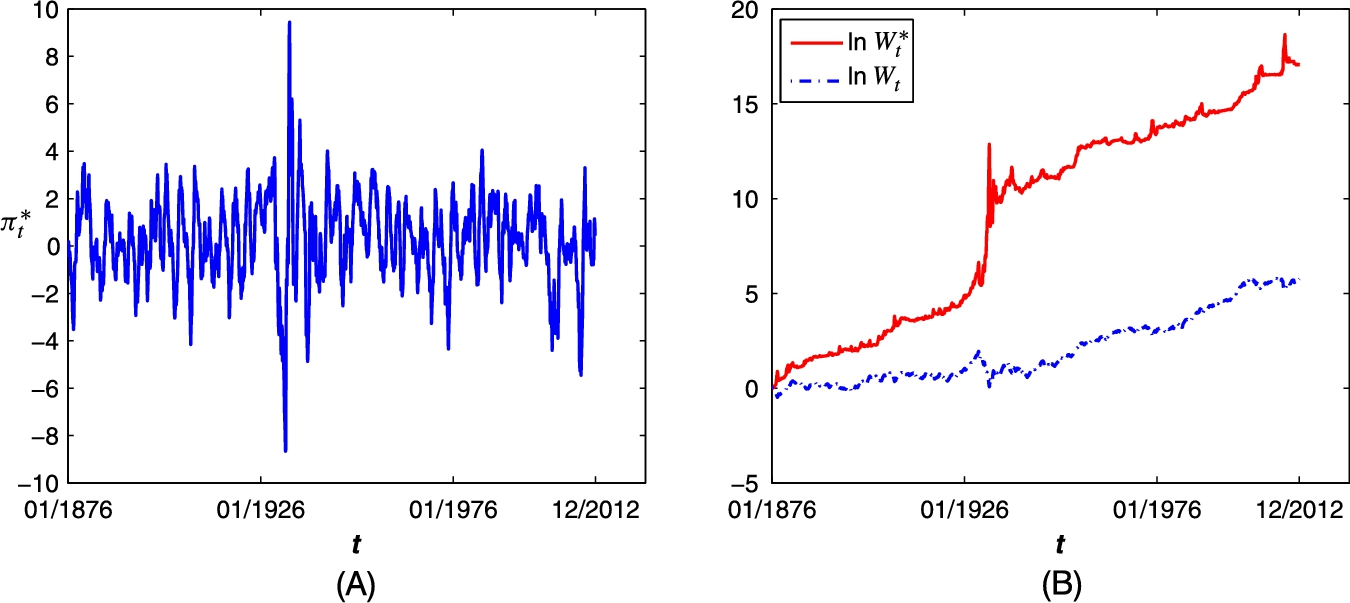
 ) from January 1876 until December 2012 for τ = 12.
4 HAMs of Multi-Asset Markets and Financial Market Interlinkages
A recent literature has been developed to understand the joint dynamics of multiple asset markets from the viewpoint of HAMs. In particular, research in this area investigates how investors' heterogeneity and changing behavior (including dynamic strategy and market selection) affect the comovement of prices, returns and volatilities in a multiple-asset framework. Modeling such interlinkages naturally introduces additional nonlinearities into HAMs and has the potential to address key issues in financial markets.
4.1 Stock Market Comovement and Policy Implications
A number of models extend the single-risky asset frameworks of Brock and Hommes (1998), Chiarella and He (2002), and Westerhoff (2003) to allow agents to switch not only across strategies but also across different asset markets. Westerhoff (2004) provides one of the first HAMs of interconnected financial markets in which both fundamentalists and chartists are simultaneously active. In each market, chartist demand is positively related to the observed price trends but negatively related to the risk of being caught in a bursting bubble. Asset prices react to the excess demand according to a log-linear price impact function. Chartists may switch between markets depending on short-run profit opportunities. The basic model of interacting agents and markets can naturally produce complex dynamics. A simple stochastic extension of the model can mimic the behavior of actual asset markets closely, offering an explanation for the high degree of stock price comovements observed empirically.
Westerhoff and Dieci (2006) extend the basic framework of Westerhoff (2004) to investigate the effect of transaction taxes when speculators can trade in two markets, and the related issue of regulatory coordination. The market fractions of fundamentalists and chartists active in each market evolve depending on the realized profitability of each ‘rule-market’ combination, which is affected by the adoption of transaction taxes. Log-price adjustments depend on excess demand and are subject to i.i.d. random noise (uncorrelated across markets). The joint dynamics of the two markets is investigated with and without transaction taxes. Moreover, the effectiveness12 of transaction taxes is assessed when tax is imposed in one market only and when uniform transaction taxes are imposed in both markets. It turns out that, while the market subject to a transaction tax becomes less distorted and less volatile, the other market may be destabilized. On the contrary, a uniform transaction tax tends to stabilize, by forcing agents to focus more strongly on fundamentals.
Building on the above frameworks, Schmitt and Westerhoff (2014) focus on coevolving stock prices in international stock markets. In their model, the demand of heterogeneous speculators is subject to different types of exogenous shocks (global shocks and shocks specific to markets or to trading rules). Investors switch between strategies and between markets depending on a number of behavioral factors and market circumstances. Besides reproducing a large number of statistical properties of stock markets (‘stylized facts’), the model shows how traders' behavior can amplify financial market interlinkages and generate stock price comovements and cross-correlations of volatilities.
Other recent papers are closely related to the above topics. For instance, Huang and Chen (2014) develop a nonlinear model with chartists and fundamentalists that generalizes the framework of Day and Huang (1990) to the case of two regional stock markets with a common currency, in order to investigate the global effects of financial market integration and of possible stabilization policies. In an agent-based model where portfolio managers allocate their funds between two asset markets, Feldman (2010) shows how fund managers' aggregate behavior can undermine global financial stability, whenever they enter the markets in large numbers, their leverage increases and their investment strategies are affected by behavioral factors (such as loss aversion). Overall, such models demonstrate the potential of HAMs for understanding the global effects of financial market interlinkages.
4.2 Heterogeneous Beliefs and Evolutionary CAPM
A further strand of research investigates the impact of behavioral heterogeneity in an evolutionary CAPM framework. More precisely, this literature adopts standard mean-variance portfolio selection across multiple assets (or asset classes/markets) and develops a dynamic CAPM framework with fundamental and technical traders. Investors update their beliefs about the means, variances and covariances of the prices or returns of the risky assets, based on fundamental information and historical prices. They may either use fixed rules (Chiarella et al., 2007, 2013a) or switch between different strategies based on their performance (Chiarella et al., 2013b). This framework is helpful to understand how investors' behavior can produce changes of the market portfolio and spillovers of volatility and correlation across markets. In particular, through the construction of a consensus belief, Chiarella et al. (2013b) develop a dynamic CAPM relationship between the market-average expected returns of the risky assets and their ex-ante betas in temporary equilibrium. Results show that systematic changes in the market portfolio and risk-return relationships may occur due to changes of investor sentiment (such as chartists acting more strongly as momentum traders). Besides providing behavioral explanations for the debated on time-varying betas, such models allow to compare theoretical ex-ante betas to commonly used ex-post beta estimates based on rolling-windows. The remainder of this section presents the model setup and key findings of Chiarella et al. (2013b).
4.2.1 A Dynamic Multi-Asset Model
Consider an economy with H agent-types, indexed by h=1,⋯,H![]() , where the agents within the same group are homogeneous in their beliefs and risk aversion. Agents invest in portfolios of a riskless asset (with a risk-free gross return Rf=1+rf
, where the agents within the same group are homogeneous in their beliefs and risk aversion. Agents invest in portfolios of a riskless asset (with a risk-free gross return Rf=1+rf![]() ) and N risky assets, indexed by j=1,⋯,N
) and N risky assets, indexed by j=1,⋯,N![]() (with N⩾1
(with N⩾1![]() ). Vectors pt=(p1,t,⋯,pN,t)⊤
). Vectors pt=(p1,t,⋯,pN,t)⊤![]() , dt=(d1,t,⋯,dN,t)⊤
, dt=(d1,t,⋯,dN,t)⊤![]() , and xt:=pt+dt
, and xt:=pt+dt![]() denote prices, dividends, and payoffs of the risky assets at time t. Assume that an agent of type h maximizes expected CARA utility, uh(w)=−e−θhw
denote prices, dividends, and payoffs of the risky assets at time t. Assume that an agent of type h maximizes expected CARA utility, uh(w)=−e−θhw![]() , of one-period-ahead wealth, where θh
, of one-period-ahead wealth, where θh![]() is the agent's absolute risk aversion coefficient. Then the optimal demand for the risky assets (in terms of number of shares) is determined as the N-dimensional vector zh,t=θ−1hΩ−1h,t[Eh,t(xt+1)−Rfpt]
is the agent's absolute risk aversion coefficient. Then the optimal demand for the risky assets (in terms of number of shares) is determined as the N-dimensional vector zh,t=θ−1hΩ−1h,t[Eh,t(xt+1)−Rfpt]![]() , where Eh,t(xt+1)
, where Eh,t(xt+1)![]() and Ωh,t=[Covh,t(xj,t+1,xk,t+1)]N×N
and Ωh,t=[Covh,t(xj,t+1,xk,t+1)]N×N![]() are the subjective conditional expectation and variance-covariance matrix of the risky payoffs. Moreover, denote by nh,t
are the subjective conditional expectation and variance-covariance matrix of the risky payoffs. Moreover, denote by nh,t![]() the market fraction of agents of type h at time t. Market clearing requires:
the market fraction of agents of type h at time t. Market clearing requires:
(17) H∑h=1nh,tzh,t=H∑h=1nh,tθ−1hΩ−1h,t[Eh,t(xt+1)−Rfpt]=zst,
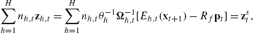
where zst=s+ξt![]() is a N-dimensional supply vector of the risky assets, subject to random supply shocks satisfying ξt=ξt−1+σκκt
is a N-dimensional supply vector of the risky assets, subject to random supply shocks satisfying ξt=ξt−1+σκκt![]() , where κt
, where κt![]() is standard normal i.i.d. with E(κt)=0
is standard normal i.i.d. with E(κt)=0![]() , Cov(κt)=I
, Cov(κt)=I![]() . Likewise, dividends dt
. Likewise, dividends dt![]() are assumed to follow a N-dimensional martingale process, dt=dt−1+σζζt
are assumed to follow a N-dimensional martingale process, dt=dt−1+σζζt![]() , where ζt
, where ζt![]() is standard normal i.i.d. with E(ζt)=0
is standard normal i.i.d. with E(ζt)=0![]() , Cov(ζt)=I
, Cov(ζt)=I![]() , independent of κt
, independent of κt![]() .13 In spite of heterogeneous beliefs about asset prices, conditional beliefs about dividends are assumed to be homogeneous across agents and correct.
.13 In spite of heterogeneous beliefs about asset prices, conditional beliefs about dividends are assumed to be homogeneous across agents and correct.
4.2.2 Price Dynamics Under Consensus Belief
Solving Eq. (17) one obtains the temporary equilibrium asset prices, pt![]() , as functions of the beliefs, risk attitudes, and current market proportions of the H agent-types. The solution can be rewritten as if prices were determined by a homogeneous agent endowed with average risk aversion θa,t:=(∑Hh=1nh,tθ−1h)−1
, as functions of the beliefs, risk attitudes, and current market proportions of the H agent-types. The solution can be rewritten as if prices were determined by a homogeneous agent endowed with average risk aversion θa,t:=(∑Hh=1nh,tθ−1h)−1![]() and a ‘consensus’ belief about the conditional first and second moments of the payoff process, {Ea,t,Ωa,t}
and a ‘consensus’ belief about the conditional first and second moments of the payoff process, {Ea,t,Ωa,t}![]() , where
, where
Ωa,t=θ−1a,t(H∑h=1nh,tθ−1hΩ−1h,t)−1,Ea,t(xt+1)=θa,tΩa,tH∑h=1nh,tθ−1hΩ−1h,tEh,t(xt+1).
From (17) and the assumption of homogeneous and correct beliefs about dividends, one obtains
(18) pt=1Rf[Ea,t(pt+1)+dt−θa,tΩa,tzst].

Eq. (18) represents pt![]() in a standard way as the discounted value of the expected end-of-period payoffs. The adjustment for the risk takes place through a negative correction to the dividends. The equilibrium prices decrease with the discount rate and increase with the expectations of future prices and dividends (other things being equal), whereas they tend to be negatively affected by risk aversion, risk perceptions, and the supply of assets.
in a standard way as the discounted value of the expected end-of-period payoffs. The adjustment for the risk takes place through a negative correction to the dividends. The equilibrium prices decrease with the discount rate and increase with the expectations of future prices and dividends (other things being equal), whereas they tend to be negatively affected by risk aversion, risk perceptions, and the supply of assets.
4.2.3 Fitness and Strategy Switching
Based on the discrete choice model adopted in HAMs, the fraction nh,t![]() of agents of type h depends on their strategy's fitness vh,t−1
of agents of type h depends on their strategy's fitness vh,t−1![]() , namely, nh,t=eηvh,t−1/Zt
, namely, nh,t=eηvh,t−1/Zt![]() , where Zt=∑heηvh,t−1
, where Zt=∑heηvh,t−1![]() and η>0
and η>0![]() is the intensity of choice. The fitness is specified as vh,t=πh,t−πBh,t−Ch
is the intensity of choice. The fitness is specified as vh,t=πh,t−πBh,t−Ch![]() , where Ch⩾0
, where Ch⩾0![]() measures the cost of the strategy, and
measures the cost of the strategy, and
(19) πh,t:=z⊤h,t−1(pt+dt−Rfpt−1)−θh2z⊤h,t−1Ωh,t−1zh,t−1,
(20) πBh,t:=(θa,t−1θhs)⊤(pt+dt−Rfpt−1)−θh2(θa,t−1θhs)⊤Ωh,t−1(θa,t−1θhs).

This performance measure generalizes the risk-adjusted profit introduced by Hommes (2001) represented by (19).14 It views strategy h as a successful strategy only to the extent that portfolio zh,t−1![]() outperforms (in terms of risk-adjusted profitability) portfolio zBh,t−1:=θa,t−1θhs
outperforms (in terms of risk-adjusted profitability) portfolio zBh,t−1:=θa,t−1θhs![]() . The latter can be naturally interpreted as a ‘benchmark’ portfolio for type-h agents, based on their risk aversion θh
. The latter can be naturally interpreted as a ‘benchmark’ portfolio for type-h agents, based on their risk aversion θh![]() .15 Moreover, as shown in Chiarella et al. (2013b), the fitness measure vh,t
.15 Moreover, as shown in Chiarella et al. (2013b), the fitness measure vh,t![]() is not affected by the differences in risk aversion across agents.
is not affected by the differences in risk aversion across agents.
4.2.4 Fundamentalists and Trend Followers
In particular, the model focuses on the interplay of fundamentalists and trend followers, indexed by h∈{f,c}![]() , respectively. Based on their beliefs in mean reversion, the price expectations of the fundamentalists are specified as Ef,t(pt+1)=pt−1+α(Ef,t(p⁎t+1)−pt−1)
, respectively. Based on their beliefs in mean reversion, the price expectations of the fundamentalists are specified as Ef,t(pt+1)=pt−1+α(Ef,t(p⁎t+1)−pt−1)![]() , where p⁎t=(p⁎1,t,⋯,p⁎N,t)
, where p⁎t=(p⁎1,t,⋯,p⁎N,t)![]() is the vector of fundamental values at time t, α:=diag[α1,⋯,αN]
is the vector of fundamental values at time t, α:=diag[α1,⋯,αN]![]() , and αj∈[0,1]
, and αj∈[0,1]![]() reflects their confidence in the fundamental price for asset j. The beliefs of the fundamentalists about the covariance matrix of the payoffs are assumed constant, Ωf,t=Ω0:=(σjk)N×N
reflects their confidence in the fundamental price for asset j. The beliefs of the fundamentalists about the covariance matrix of the payoffs are assumed constant, Ωf,t=Ω0:=(σjk)N×N![]() . Fundamental prices p⁎t
. Fundamental prices p⁎t![]() are assumed to evolve exogenously as a martingale process, consistent with the assumed dividend and supply processes. Moreover, p⁎t
are assumed to evolve exogenously as a martingale process, consistent with the assumed dividend and supply processes. Moreover, p⁎t![]() is also consistent with Eq. (18) under the special case of homogeneous and correct first-moment beliefs, constant risk aversion ‾θ
is also consistent with Eq. (18) under the special case of homogeneous and correct first-moment beliefs, constant risk aversion ‾θ![]() , and constant second moment beliefs Ω0
, and constant second moment beliefs Ω0![]() . This results in
. This results in
(21) p⁎t=1rf(dt−‾θΩ0(s+ξt)),
which implies p⁎t+1=p⁎t+ϵt+1![]() , where ϵt+1:=1rf(σζζt+1−‾θΩ0σκκt+1)∼
, where ϵt+1:=1rf(σζζt+1−‾θΩ0σκκt+1)∼![]() i.i.d. normal. The fundamental price process can be treated as ‘steady state’ of the dynamic heterogeneous-belief model.
i.i.d. normal. The fundamental price process can be treated as ‘steady state’ of the dynamic heterogeneous-belief model.
Unlike the fundamentalists, trend followers form their beliefs about price trends based on the observed prices and (exponential) moving averages. Their conditional mean and covariance matrices are assumed to satisfy Ec,t(pt+1)=pt−1+γ(pt−1−ut−1)![]() , Ωc,t=Ω0+λVt−1
, Ωc,t=Ω0+λVt−1![]() , where ut−1
, where ut−1![]() and Vt−1
and Vt−1![]() are sample means and covariance matrices of historical prices pt−1,pt−2,⋯
are sample means and covariance matrices of historical prices pt−1,pt−2,⋯![]() . Moreover, γ=diag[γ1,⋯,γN]>0
. Moreover, γ=diag[γ1,⋯,γN]>0![]() , γj
, γj![]() measures the ‘strength’ of extrapolation for asset j, and λ measures the sensitivity of the second-moment estimate to the sample variance. Quantities ut
measures the ‘strength’ of extrapolation for asset j, and λ measures the sensitivity of the second-moment estimate to the sample variance. Quantities ut![]() and Vt
and Vt![]() are updated recursively according to ut=δut−1+(1−δ)pt
are updated recursively according to ut=δut−1+(1−δ)pt![]() and Vt=δVt−1+δ(1−δ)(pt−ut−1)(pt−ut−1)⊤
and Vt=δVt−1+δ(1−δ)(pt−ut−1)(pt−ut−1)⊤![]() , where parameter δ∈[0,1]
, where parameter δ∈[0,1]![]() is related to the weight of past information.
is related to the weight of past information.
The optimal portfolios of fundamentalists and chartists are then given by, respectively,
(22) zf,t=θ−1fΩ−10[pt−1+dt+α(p⁎t−pt−1)−Rfpt],
(23) zc,t=θ−1c[Ω0+λVt−1]−1[pt−1+dt+γ(pt−1−ut−1)−Rfpt].
4.2.5 Dynamic Model and Stability Properties
The stochastic nonlinear multi-asset HAM with two belief-types results in the following recursive equation for asset prices
(24) pt=θa,tRfΩa,t[nf,tθfΩ−10(pt−1+α(p⁎t−pt−1))+nc,tθc(Ω0+λVt−1)−1(pt−1+γ(pt−1−ut−1))−s−ξt]+1Rfdt,

where the average risk aversion and second-moment beliefs satisfy θa,t=(nf,tθf+nc,tθc)−1![]() and Ωa,t=1θa,t(nf,tθfΩ−10+nc,tθc(Ω0+λVt−1)−1)−1
and Ωa,t=1θa,t(nf,tθfΩ−10+nc,tθc(Ω0+λVt−1)−1)−1![]() . In (24), market fractions evolve based on performances vf,t−1
. In (24), market fractions evolve based on performances vf,t−1![]() and vc,t−1
and vc,t−1![]() , as follows:
, as follows:
nf,t=11+e−η(vf,t−1−vc,t−1), nc,t=1−nf,t,
where
vf,t=(zf,t−1−θa,t−1sθf)⊤[pt+dt−Rfpt−1−θf2Ω0(zf,t−1+θa,t−1sθf)]−Cf,vc,t=(zc,t−1−θa,t−1sθc)⊤×[pt+dt−Rfpt−1−θc2(Ω0+λVt−2)(zc,t−1+θa,t−1sθc)]−Cc,
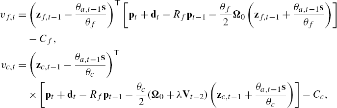
and Cf⩾Cc⩾0![]() .
.
Despite the large dimension of the dynamical system, insightful analytical results about the steady state and its stability properties are possible for the ‘deterministic skeleton’, obtained by setting the supply and dividends at their unconditional mean levels ξt=0![]() , dt=ˉd
, dt=ˉd![]() . The model admits a unique steady state16 (pt,ut,Vt,nf,t)=(p⁎,p⁎,0,n⁎f):=F⁎
. The model admits a unique steady state16 (pt,ut,Vt,nf,t)=(p⁎,p⁎,0,n⁎f):=F⁎![]() , where p⁎=1rf(ˉd−θ⁎aΩ0s)
, where p⁎=1rf(ˉd−θ⁎aΩ0s)![]() is the fundamental price vector of the deterministic system, θ⁎a=1/(n⁎f/θf+n⁎c/θc)
is the fundamental price vector of the deterministic system, θ⁎a=1/(n⁎f/θf+n⁎c/θc)![]() is the average risk aversion and n⁎f=1/(1+eη(Cf−Cc))
is the average risk aversion and n⁎f=1/(1+eη(Cf−Cc))![]() , n⁎c=1−n⁎f
, n⁎c=1−n⁎f![]() are the market fractions of the fundamentalist and chartist, respectively, at the steady state. It turns out that the local stability of F⁎
are the market fractions of the fundamentalist and chartist, respectively, at the steady state. It turns out that the local stability of F⁎![]() is based on clear-cut and intuitive analytical relationships between chartist extrapolation and memory, fundamentalist confidence, and switching intensity. We set θ0:=θf/θc
is based on clear-cut and intuitive analytical relationships between chartist extrapolation and memory, fundamentalist confidence, and switching intensity. We set θ0:=θf/θc![]() , CΔ:=Cf−Cc
, CΔ:=Cf−Cc![]() , and denote by Jo⊆{1,⋯,N}
, and denote by Jo⊆{1,⋯,N}![]() the subset of assets characterized by ‘sufficiently’ strong extrapolation from the chartists, namely, by γj>Rf/δ−1
the subset of assets characterized by ‘sufficiently’ strong extrapolation from the chartists, namely, by γj>Rf/δ−1![]() . In the typical case CΔ>0
. In the typical case CΔ>0![]() , the local stability results can be summarized as follows:
, the local stability results can be summarized as follows:
- (i) If the chartist extrapolation is not very strong in general (namely, γj⩽Rf/δ−1
 for all j∈{1,⋯,N}
 ), the steady state F⁎
 is locally stable for any level of the switching intensity η;
 - (ii) If chartist extrapolation is sufficiently strong for some (possibly for all) assets (Jo≠∅
 ), then F⁎ is locally stable when the switching intensity is not too strong, namely η<ˆηm:=minj∈Joˆηj
 , where ˆηj
 for asset j is defined by
(25) ˆηj:=1CΔlnRf−δ(1−αj)θ0[δ(1+γj)−Rf].

- Moreover, for increasing switching intensity F⁎ undergoes a Neimark–Sacker bifurcation at η=ˆηm
 .
.
Roughly speaking, investors' switching intensity η is not sufficient, per se, to destabilize the steady state F⁎![]() (case (i)), but the possibility that investors' behavior destabilizes the system depends on the joint effect of the switching intensity η and the chartists' strengths of extrapolation γj
(case (i)), but the possibility that investors' behavior destabilizes the system depends on the joint effect of the switching intensity η and the chartists' strengths of extrapolation γj![]() , j=1,2,…,N
, j=1,2,…,N![]() . In case (ii), the threshold ˆηj
. In case (ii), the threshold ˆηj![]() is determined for each asset according to (25), depending, amongst others, negatively on γj
is determined for each asset according to (25), depending, amongst others, negatively on γj![]() and positively on αj
and positively on αj![]() . Hence, even when chartist extrapolation is strong enough for some asset j (so that γj>Rf/δ−1
. Hence, even when chartist extrapolation is strong enough for some asset j (so that γj>Rf/δ−1![]() ), the system can still be stable when the fundamentalists dominate the market at the steady state and the switching intensity is not too large. Conversely, since the stability depends on the lowest threshold amongst assets (ˆηm
), the system can still be stable when the fundamentalists dominate the market at the steady state and the switching intensity is not too large. Conversely, since the stability depends on the lowest threshold amongst assets (ˆηm![]() ), a large extrapolation on one or few assets is sufficient for the whole system to be eventually destabilized for large enough η. Numerical investigations confirm that, by increasing η in case (ii), fluctuations are initially ‘confined’ to the asset with the lowest ˆηj
), a large extrapolation on one or few assets is sufficient for the whole system to be eventually destabilized for large enough η. Numerical investigations confirm that, by increasing η in case (ii), fluctuations are initially ‘confined’ to the asset with the lowest ˆηj![]() and then spill over to the whole system of interconnected assets. As for the ‘non asset-specific’ parameters, the above results show that increases in δ, Cf
and then spill over to the whole system of interconnected assets. As for the ‘non asset-specific’ parameters, the above results show that increases in δ, Cf![]() , and θf
, and θf![]() (respectively Rf
(respectively Rf![]() , Cc
, Cc![]() , and θc
, and θc![]() ) tend to reduce (respectively to increase) all thresholds ˆηj
) tend to reduce (respectively to increase) all thresholds ˆηj![]() , j=1,2,...,N
, j=1,2,...,N![]() . In particular, larger values of the ratio θ0=θf/θc
. In particular, larger values of the ratio θ0=θf/θc![]() of the fundamentalist and chartist risk aversion and of the strategy cost differential CΔ=Cf−Cc
of the fundamentalist and chartist risk aversion and of the strategy cost differential CΔ=Cf−Cc![]() reduce the stability domain, whereas a larger risk-free return Rf
reduce the stability domain, whereas a larger risk-free return Rf![]() or a faster decay in chartist moving averages (i.e. a smaller δ) widens the stability domain.
or a faster decay in chartist moving averages (i.e. a smaller δ) widens the stability domain.
4.2.6 Nonlinear Risk-Return Patterns
Further results concern the impact of the dynamic correlation structure on the global properties of the stochastic model. Although the levels of the fundamental prices do depend on the ‘exogenous’ subjective beliefs about variances and covariances, Ω0![]() , such beliefs have no influence on the local stability properties.17 However, second-moment beliefs and their evolution turn out to be very important for the dynamics of the nonlinear system buffeted by exogenous noise. The nonlinear stochastic model is characterized by emerging patterns and systematic changes in risk-return relationships that can by no means be explained by the linearized model. One important example concerns the nonlinear stochastic nature of the time-varying ex-ante beta coefficients implied by the model (based on the consensus beliefs), and of the realized betas, estimated using rolling windows.18 The value at time t and the payoff at time t+1
, such beliefs have no influence on the local stability properties.17 However, second-moment beliefs and their evolution turn out to be very important for the dynamics of the nonlinear system buffeted by exogenous noise. The nonlinear stochastic model is characterized by emerging patterns and systematic changes in risk-return relationships that can by no means be explained by the linearized model. One important example concerns the nonlinear stochastic nature of the time-varying ex-ante beta coefficients implied by the model (based on the consensus beliefs), and of the realized betas, estimated using rolling windows.18 The value at time t and the payoff at time t+1![]() of the market portfolio are given by Wm,t=p⊤ts
of the market portfolio are given by Wm,t=p⊤ts![]() and Wm,t+1=x⊤t+1s
and Wm,t+1=x⊤t+1s![]() , respectively, while rj,t+1=xj,t+1/pj,t−1
, respectively, while rj,t+1=xj,t+1/pj,t−1![]() , rm,t+1=Wm,t+1/Wm,t−1
, rm,t+1=Wm,t+1/Wm,t−1![]() represent the returns of risky asset j and of the market portfolio, respectively. Hence, under the consensus belief, Ea,t(Wm,t+1)=Ea,t(xt+1)⊤s
represent the returns of risky asset j and of the market portfolio, respectively. Hence, under the consensus belief, Ea,t(Wm,t+1)=Ea,t(xt+1)⊤s![]() , Vara,t(Wm,t+1)=s⊤Ωa,ts
, Vara,t(Wm,t+1)=s⊤Ωa,ts![]() , Ea,t(rj,t+1)=Ea,t(xj,t+1)pj,t−1
, Ea,t(rj,t+1)=Ea,t(xj,t+1)pj,t−1![]() , Ea,t(rm,t+1)=Ea,t(Wm,t+1)Wm,t−1
, Ea,t(rm,t+1)=Ea,t(Wm,t+1)Wm,t−1![]() . Following Chiarella et al. (2011), one obtains the CAPM-like return relation19
. Following Chiarella et al. (2011), one obtains the CAPM-like return relation19
(26) Ea,t(rt+1)−rf1=βa,t[Ea,t(rm,t+1)−rf],
where rt+1![]() is the vector collecting the risky returns and βa,t=(β1,t,⋯,βN,t)⊤
is the vector collecting the risky returns and βa,t=(β1,t,⋯,βN,t)⊤![]() , βj,t=Cova,t(rm,t+1,rj,t+1)Vara,t(rm,t+1)
, βj,t=Cova,t(rm,t+1,rj,t+1)Vara,t(rm,t+1)![]() are the ex-ante beta coefficients, in the sense that they reflect the temporary market equilibrium condition under the consensus beliefs Ea,t
are the ex-ante beta coefficients, in the sense that they reflect the temporary market equilibrium condition under the consensus beliefs Ea,t![]() and Ωa,t
and Ωa,t![]() . In the case of two risky assets, Fig. 8 (from the top-left to bottom-right) shows the time series of asset prices (pt
. In the case of two risky assets, Fig. 8 (from the top-left to bottom-right) shows the time series of asset prices (pt![]() ), asset returns (rt
), asset returns (rt![]() ), the aggregate wealth shares invested in the risky assets (i.e. the market portfolio weights, denoted as ωt:=(ω1,t,ω2,t)⊤
), the aggregate wealth shares invested in the risky assets (i.e. the market portfolio weights, denoted as ωt:=(ω1,t,ω2,t)⊤![]() ), the ex-ante betas of the risky assets under the consensus belief (βa,t
), the ex-ante betas of the risky assets under the consensus belief (βa,t![]() ), and the estimates of the betas using rolling windows of 100 and of 300 periods.20 In particular, the variation of the ex-ante beta coefficients is significant and seems to indicate substantially different levels over different subperiods. Although the rolling estimates of the betas do not necessarily reflect the nature of the ex-ante betas implied by the CAPM (see also Chiarella et al., 2013a), the 100-period and the (smoother) 300-period rolling betas also reveal systematic changes in risk-return relationships, with patterns similar to the ex-ante betas.
), and the estimates of the betas using rolling windows of 100 and of 300 periods.20 In particular, the variation of the ex-ante beta coefficients is significant and seems to indicate substantially different levels over different subperiods. Although the rolling estimates of the betas do not necessarily reflect the nature of the ex-ante betas implied by the CAPM (see also Chiarella et al., 2013a), the 100-period and the (smoother) 300-period rolling betas also reveal systematic changes in risk-return relationships, with patterns similar to the ex-ante betas.
Finally, further numerical results on the relationship between trading volume and volatility indicate that the ACs for both volatility and trading volume are highly significant and decaying over long lags, which is close to what we have observed in financial markets. Moreover, the correlation between price volatility and trading volume of the risky assets is remarkably influenced by the assets' correlation structure.
From a broader perspective, the results described in this section are part of a growing stream of research. They show that asset diversification in a dynamic setting where investors rebalance their portfolios based on heterogeneous strategies and behavioral rules may produce aggregate effects that different substantially from risk reduction and equilibrium risk-return relationships predicted by standard mean-variance analysis and finance theory. Amongst recent work in this area, Brock et al. (2009) show that the introduction of additional hedging instruments in the baseline asset pricing setup of Brock and Hommes (1998) may have destabilizing effects in the presence of heterogeneity and adaptive behavior according to performance-based reinforcement learning. In an evolutionary finance setting that allows for the coexistence of different trading strategies, the stochastic multi-asset model of Anufriev et al. (2012) shows the existence of strong trading-induced excess covariance in equilibrium, which is a key ingredient of systemic risk. Corsi et al. (2016) investigate the dynamic effect of financial innovation and increasing diversification in a model of heterogeneous financial institutions subject to Value-at-Risk constraints. They show that this may lead to systemic instabilities, through increased leverage and overlapping portfolios. Similar channels of contagion and systemic risk in financial networks are investigated by Caccioli et al. (2015).
4.3 Interacting Stock Market and Foreign Exchange Market
The recent work of Dieci and Westerhoff (2010) and Dieci and Westerhoff (2013b) investigates how the trading activity of foreign-based stock market speculators – who care both about stock returns and exchange rate movements – can affect otherwise independent stock markets denominated in different currencies and the related foreign exchange market. We brief the main findings in the following.
Let us abstract from the impact of international trade on exchange rates, and focus on the sole effect of financial market speculators. For simplicity, let us define cross-market traders the investors from one country who are active in the stock market of the other country, in contrast to home-market traders.21 Quantities Pt![]() , Qt
, Qt![]() , and St
, and St![]() denote the price of the domestic asset (in domestic currency), the price of the foreign asset (in foreign currency) and the exchange rate,22 while P⁎
denote the price of the domestic asset (in domestic currency), the price of the foreign asset (in foreign currency) and the exchange rate,22 while P⁎![]() , Q⁎
, Q⁎![]() , and S⁎
, and S⁎![]() denote their fundamental values, respectively. We use lowercase letters for log-prices pt
denote their fundamental values, respectively. We use lowercase letters for log-prices pt![]() , qt
, qt![]() , st
, st![]() , p⁎
, p⁎![]() , q⁎
, q⁎![]() , s⁎
, s⁎![]() , respectively.
, respectively.
Exchange rate movements are driven by the excess demand for domestic currency. As such, they are directly affected by foreign exchange speculators, but they also depend, indirectly, on stock transactions of cross-market traders. This is captured by:
(27) st+1−st=αS(Ut+Xt+Yt),αS>0,
where (positive or negative) quantities Ut![]() , Xt
, Xt![]() , and Yt
, and Yt![]() are different components of the excess demand for domestic currency, expressed in currency units. More precisely, Ut
are different components of the excess demand for domestic currency, expressed in currency units. More precisely, Ut![]() is the excess demand for domestic currency due to direct speculation in the foreign exchange market (to be specified later), Xt:=Pt˜Dt=˜Dtexp(pt)
is the excess demand for domestic currency due to direct speculation in the foreign exchange market (to be specified later), Xt:=Pt˜Dt=˜Dtexp(pt)![]() is the currency excess demand from foreign traders active in the domestic stock market (and demanding/supplying ˜Dt
is the currency excess demand from foreign traders active in the domestic stock market (and demanding/supplying ˜Dt![]() units of domestic asset), and Yt:=−Qt˜Zt/St=−˜Ztexp(qt−st)
units of domestic asset), and Yt:=−Qt˜Zt/St=−˜Ztexp(qt−st)![]() is the excess demand generated by domestic traders active in the foreign stock market (since ˜Zt
is the excess demand generated by domestic traders active in the foreign stock market (since ˜Zt![]() units of foreign stock correspond to Qt˜Zt
units of foreign stock correspond to Qt˜Zt![]() units of foreign currency and thus result in a counter transaction of −Qt˜Zt/St
units of foreign currency and thus result in a counter transaction of −Qt˜Zt/St![]() units of domestic currency).
units of domestic currency).
Similar price adjustment mechanisms are assumed for the two stock markets:
(28) pt+1−pt=αPDEt,qt+1−qt=αQZEt,αP,αQ>0
where DEt![]() and ZEt
and ZEt![]() denote the excess demand for the domestic and foreign stock, respectively, including the components ˜Dt
denote the excess demand for the domestic and foreign stock, respectively, including the components ˜Dt![]() and ˜Zt
and ˜Zt![]() from cross-market traders, as explained below. In a framework with two agent-types, both DEt
from cross-market traders, as explained below. In a framework with two agent-types, both DEt![]() and ZEt
and ZEt![]() can be modeled as the sum of four components, representing the demand of domestic and foreign chartists and fundamentalists. At time t, the excess demand DEt
can be modeled as the sum of four components, representing the demand of domestic and foreign chartists and fundamentalists. At time t, the excess demand DEt![]() for the domestic asset is given by:
for the domestic asset is given by:
(29) DEt=β(pt−pt−1)+θ(p⁎−pt)+˜Dt,
where ˜Dt=˜β(st+pt−st−1−pt−1)+˜θ(s⁎−st+p⁎−pt)![]() and β,θ,˜β,˜θ⩾0
and β,θ,˜β,˜θ⩾0![]() . Both β(pt−pt−1)
. Both β(pt−pt−1)![]() and θ(p⁎−pt)
and θ(p⁎−pt)![]() represent the demand from domestic chartists and fundamentalists, based on the observed price trend and the observed mispricing, respectively. Similar comments hold for demands ˜β(st+pt−st−1−pt−1)
represent the demand from domestic chartists and fundamentalists, based on the observed price trend and the observed mispricing, respectively. Similar comments hold for demands ˜β(st+pt−st−1−pt−1)![]() and ˜θ(s⁎−st+p⁎−pt)
and ˜θ(s⁎−st+p⁎−pt)![]() from foreign chartists and fundamentalists, respectively, which depend also on the observed trend and misalignment of the exchange rate. Symmetrically, demand ZEt
from foreign chartists and fundamentalists, respectively, which depend also on the observed trend and misalignment of the exchange rate. Symmetrically, demand ZEt![]() for the foreign asset is given by:
for the foreign asset is given by:
(30) ZEt=γ(qt−qt−1)+ψ(q⁎−qt)+˜Zt,
where ˜Zt=˜γ(−st+qt+st−1−qt−1)+˜ψ(−s⁎+st+q⁎−qt)![]() and γ,ψ,˜γ,˜ψ⩾0
and γ,ψ,˜γ,˜ψ⩾0![]() . The four terms γ(qt−qt−1)
. The four terms γ(qt−qt−1)![]() , ψ(q⁎−qt)
, ψ(q⁎−qt)![]() , ˜γ(−st+qt+st−1−qt−1)
, ˜γ(−st+qt+st−1−qt−1)![]() and ˜ψ(−s⁎+st+q⁎−qt)
and ˜ψ(−s⁎+st+q⁎−qt)![]() represent the demands from foreign chartists, foreign fundamentalists, domestic chartists and domestic fundamentalists, respectively.
represent the demands from foreign chartists, foreign fundamentalists, domestic chartists and domestic fundamentalists, respectively.
Dieci and Westerhoff (2013b) investigate the case without foreign exchange speculators (Ut≡0![]() in Eq. (27)). Even if demand in the stock markets is linear in (log-)prices, the joint dynamics (27)–(30) of the three markets results in a nonlinear dynamical system, by construction, due to the products, ‘price×quantity’, which govern the exchange rate dynamics (27).23 Moreover, although system (27)–(30) is 6-dimensional, analytical stability conditions of the unique ‘fundamental’ steady state (FSS henceforth)24 can be derived in the case of symmetric markets, namely, β=γ
in Eq. (27)). Even if demand in the stock markets is linear in (log-)prices, the joint dynamics (27)–(30) of the three markets results in a nonlinear dynamical system, by construction, due to the products, ‘price×quantity’, which govern the exchange rate dynamics (27).23 Moreover, although system (27)–(30) is 6-dimensional, analytical stability conditions of the unique ‘fundamental’ steady state (FSS henceforth)24 can be derived in the case of symmetric markets, namely, β=γ![]() , ˜β=˜γ
, ˜β=˜γ![]() , θ=ψ
, θ=ψ![]() , ˜θ=˜ψ
, ˜θ=˜ψ![]() , q⁎=p⁎+s⁎
, q⁎=p⁎+s⁎![]() , thanks to a factorization of the characteristic polynomial of the Jacobian matrix at the FSS. This allows an exhaustive comparison of the stability condition for the integrated system with that of otherwise independent stock markets.
, thanks to a factorization of the characteristic polynomial of the Jacobian matrix at the FSS. This allows an exhaustive comparison of the stability condition for the integrated system with that of otherwise independent stock markets.
Fig. 9 illustrates the impact of parameters ˜β![]() and ˜θ
and ˜θ![]() of the cross-market traders on the stability of the steady state of otherwise independent symmetric stock markets. The stability region is represented in the plane of parameters β and θ of home-market traders. In both panels, the area bounded by the axes and by the two (thick) lines of equations θ=2(1+β)
of the cross-market traders on the stability of the steady state of otherwise independent symmetric stock markets. The stability region is represented in the plane of parameters β and θ of home-market traders. In both panels, the area bounded by the axes and by the two (thick) lines of equations θ=2(1+β)![]() and β=1
and β=1![]() is the stability region for isolated symmetric markets, which we denote by S
is the stability region for isolated symmetric markets, which we denote by S![]() . Therefore, the markets in isolation may become unstable in the presence of sufficiently large chartist extrapolation (β) or fundamentalist reaction (θ) from the home-market traders. If the two markets interact (˜β,˜θ≠0
. Therefore, the markets in isolation may become unstable in the presence of sufficiently large chartist extrapolation (β) or fundamentalist reaction (θ) from the home-market traders. If the two markets interact (˜β,˜θ≠0![]() ), the FSS of the resulting integrated system is unstable for at least all the parameter combinations (β,θ
), the FSS of the resulting integrated system is unstable for at least all the parameter combinations (β,θ![]() ) originally in area S
) originally in area S![]() and now falling within the dark grey region, say area R⊂S
and now falling within the dark grey region, say area R⊂S![]() . The shape and extension of area R
. The shape and extension of area R![]() depend on the behavioral parameters of the cross-market chartists and fundamentalists, ˜β
depend on the behavioral parameters of the cross-market chartists and fundamentalists, ˜β![]() and ˜θ
and ˜θ![]() . In particular, a larger chartist impact ˜β
. In particular, a larger chartist impact ˜β![]() tends to enlarge area R
tends to enlarge area R![]() . The left panel depicts the case ˜β<˜θ/2
. The left panel depicts the case ˜β<˜θ/2![]() , in which the integration is always destabilizing (the new stability area is strictly a subset of the original one). A destabilizing effect prevails also in the opposite case, as shown in the right panel, for ˜β⩾˜θ/2
, in which the integration is always destabilizing (the new stability area is strictly a subset of the original one). A destabilizing effect prevails also in the opposite case, as shown in the right panel, for ˜β⩾˜θ/2![]() . However, in this case there exists a parameter region (light grey area) in which the otherwise unstable isolated markets (due to overreaction of fundamentalists) may be stabilized by strong extrapolation of the cross-market traders.
. However, in this case there exists a parameter region (light grey area) in which the otherwise unstable isolated markets (due to overreaction of fundamentalists) may be stabilized by strong extrapolation of the cross-market traders.
 . Right panel: case ˜β⩾˜θ/2
 .
.We may interpret parameters β and θ as proportional to the total number of chartists and fundamentalists trading in their home markets, while ˜β![]() and ˜θ
and ˜θ![]() represent the number of additional cross-market traders of the two types. From this standpoint, the above results indicate a destabilizing effect of the market entry of additional cross-market speculators, once the two stock markets become interconnected. In addition, an even stronger result holds in the case of simple relocation of the existing mass of speculators across the markets, namely, the case when the total population of chartists (β+˜β
represent the number of additional cross-market traders of the two types. From this standpoint, the above results indicate a destabilizing effect of the market entry of additional cross-market speculators, once the two stock markets become interconnected. In addition, an even stronger result holds in the case of simple relocation of the existing mass of speculators across the markets, namely, the case when the total population of chartists (β+˜β![]() ) and fundamentalists (θ+˜θ
) and fundamentalists (θ+˜θ![]() ) remains unchanged, while parameters ˜β
) remains unchanged, while parameters ˜β![]() , ˜θ
, ˜θ![]() are increased (and β, θ are decreased accordingly). In this case the stability conditions for the integrated system are definitely more restrictive than for the markets in isolation, as proven in Dieci and Westerhoff (2013b). Further numerical investigations show the robustness of such results to the introduction of asymmetries between the two stock markets.
are increased (and β, θ are decreased accordingly). In this case the stability conditions for the integrated system are definitely more restrictive than for the markets in isolation, as proven in Dieci and Westerhoff (2013b). Further numerical investigations show the robustness of such results to the introduction of asymmetries between the two stock markets.
In a related paper, Dieci and Westerhoff (2010) investigate the case in which instability originates in the foreign exchange market due to speculative currency trading, and then it propagates to the stock markets. Different from Dieci and Westerhoff (2013b), only the fundamental traders are active in the two stock markets, while the foreign exchange market is populated by the speculators who switch between two behavioral rules, based on extrapolative and regressive beliefs, depending on the exchange rate misalignment. Therefore, the general setup (27)–(30) is reduced to a special case where β=˜β=γ=˜γ=0![]() , whereas currency excess demand Ut
, whereas currency excess demand Ut![]() is specified as:
is specified as:
(31) Ut=nc,tDFXc,t+(1−nc,t)DFXf,t,
(32) DFXc,t=κ(st−s⁎),DFXf,t=φ(s⁎−st),nc,t=[1+ν(s⁎−st)2]−1,
where κ,φ,ν>0![]() and nc,t
and nc,t![]() is the weight of extrapolative beliefs in period t. By Eqs. (31) and (32), chartist and fundamentalist demand are then proportional to the current exchange rate deviation. That is, the chartists believe that the observed misalignment will increase further, whereas the fundamentalists believe that the exchange rate will revert to the fundamental. However, the more the exchange rate deviates from its fundamental value, the more regressive beliefs gain in popularity at the expense of extrapolative beliefs, as speculators perceive the risk that the bull or bear market might collapse. Moreover, the higher parameter ν is in (32), the more sensitive the mass of speculators becomes with regard to a given misalignment.25 Intuitively, when considered in isolation (˜θ=˜ψ=0
is the weight of extrapolative beliefs in period t. By Eqs. (31) and (32), chartist and fundamentalist demand are then proportional to the current exchange rate deviation. That is, the chartists believe that the observed misalignment will increase further, whereas the fundamentalists believe that the exchange rate will revert to the fundamental. However, the more the exchange rate deviates from its fundamental value, the more regressive beliefs gain in popularity at the expense of extrapolative beliefs, as speculators perceive the risk that the bull or bear market might collapse. Moreover, the higher parameter ν is in (32), the more sensitive the mass of speculators becomes with regard to a given misalignment.25 Intuitively, when considered in isolation (˜θ=˜ψ=0![]() ), the foreign exchange market is unstable (since the extrapolative beliefs prevail and tend to increase the misalignment if st
), the foreign exchange market is unstable (since the extrapolative beliefs prevail and tend to increase the misalignment if st![]() is sufficiently close to s⁎
is sufficiently close to s⁎![]() ), whereas the two stock markets converge to their fundamental prices, thanks to the stabilizing activity of fundamental traders.
), whereas the two stock markets converge to their fundamental prices, thanks to the stabilizing activity of fundamental traders.
Dieci and Westerhoff (2010) investigate the dynamics under market integration, which results in a 3-dimensional nonlinear dynamical system, having two additional non-fundamental steady states (NFSS), beside the FSS. Analytical conditions for the FSS to be locally stable can be derived in terms of the model parameters and compared with the stability conditions of each market, considered in isolation. Bifurcation diagrams are particularly useful to understand how the ‘strength’ of the interaction between the stock markets (captured by parameters ˜θ![]() and ˜ψ
and ˜ψ![]() ) and chartist extrapolation in the foreign exchange market (parameter κ) jointly affect the stability properties. In the left panels of Fig. 10, the asymptotic behavior of the domestic (log-)stock price p (top) and (log-)exchange rate s (bottom) is plotted against extrapolation parameter κ. In the no-interaction case (illustrated by the superimposed dashed lines), the fundamental (log-)exchange rate s⁎
) and chartist extrapolation in the foreign exchange market (parameter κ) jointly affect the stability properties. In the left panels of Fig. 10, the asymptotic behavior of the domestic (log-)stock price p (top) and (log-)exchange rate s (bottom) is plotted against extrapolation parameter κ. In the no-interaction case (illustrated by the superimposed dashed lines), the fundamental (log-)exchange rate s⁎![]() is unstable and the exchange rate misalignment in the NFSS increases with κ, whereas the fundamental (log-)prices in the stock markets, p⁎
is unstable and the exchange rate misalignment in the NFSS increases with κ, whereas the fundamental (log-)prices in the stock markets, p⁎![]() and q⁎
and q⁎![]() , are stable. The plots show that the connection with stable stock markets can be beneficial, to some extent, by bringing the exchange rate back to its fundamental value (for κ<ˆκ≈0.6015
, are stable. The plots show that the connection with stable stock markets can be beneficial, to some extent, by bringing the exchange rate back to its fundamental value (for κ<ˆκ≈0.6015![]() ), or by reducing such misalignments. However, if κ is large enough, the integration can destabilize the stock markets, too, and introduce cyclical and chaotic behavior in the whole system of the interacting markets, with fluctuations of increasing amplitude. In particular, for κ>κ⁎≈4.856
), or by reducing such misalignments. However, if κ is large enough, the integration can destabilize the stock markets, too, and introduce cyclical and chaotic behavior in the whole system of the interacting markets, with fluctuations of increasing amplitude. In particular, for κ>κ⁎≈4.856![]() , the fluctuations range across a much wider area than for κ<κ⁎
, the fluctuations range across a much wider area than for κ<κ⁎![]() . While for κ<κ⁎
. While for κ<κ⁎![]() , two different attractors coexist, implying that the asymptotic dynamics of prices and exchange rate are confined to different regions depending on the initial condition (‘bull’ or ‘bear’ markets), at κ=κ⁎
, two different attractors coexist, implying that the asymptotic dynamics of prices and exchange rate are confined to different regions depending on the initial condition (‘bull’ or ‘bear’ markets), at κ=κ⁎![]() they merge into a unique attractor (through a homoclinic bifurcation).26 The right panels of Fig. 10 represent the fluctuations of p (top) and s (bottom) for very large κ, characterized by sudden switching between bull and bear markets. The dynamic analysis thus reveals a double-edged effect of market interlinkages, where behavioral factors appear to play a substantial role.
they merge into a unique attractor (through a homoclinic bifurcation).26 The right panels of Fig. 10 represent the fluctuations of p (top) and s (bottom) for very large κ, characterized by sudden switching between bull and bear markets. The dynamic analysis thus reveals a double-edged effect of market interlinkages, where behavioral factors appear to play a substantial role.

 , φ = 0.8, ν = 10000 and (in the right panels) κ = 5.3.
The interaction of foreign and domestic investors using heterogeneous trading rules, and its effect on the dynamics of the foreign exchange market, has been the subject of further research in recent years. Amongst others, Kirman et al. (2007) show that the mere interplay of speculative traders with wealth measured in two different currencies and buying or selling assets of both countries can produce bubbles in foreign exchange market and realistic features of the exchange rate series. Corona et al. (2008) develop and investigate a computationally oriented agent-based model of two stock markets and a related foreign exchange market. They focus, in particular, on the resulting volatility, covariance and correlation of the stock markets, both during quiet periods and during a monetary crisis. Overall, such models highlight a number of dynamic features that are intrinsic to a system of asset markets linked via and with foreign exchange market and that simply arise from the structural properties of such interlinkages combined with the behavior of heterogeneous traders.
5 HAMs and House Price Dynamics
This section surveys recent research on the impact of investors' behavioral heterogeneity on the dynamics of house prices and markets. Similarly to financial market dynamics, the main body of literature on house price dynamics relies on the theoretical framework of fully rational and forward looking investors (see, e.g. Poterba, 1984, Poterba et al., 1991, Clayton, 1996, Glaeser and Gyourko, 2007, Brunnermeier and Julliard, 2008). Broadly speaking, in this framework house price movements are due to sequences of exogenous shocks affecting the fundamentals of the housing market (rents, population growth, the user cost of capital, etc.), and to the resulting ‘well-behaved’ adjustments to new long-run equilibrium levels. Real estate market efficiency is an implication of such rationality assumptions.
Despite the remarkable achievements in this literature, a number of housing market phenomena are far from being fully understood. This includes the existence of boom-bust housing cycles unrelated to changes in underlying fundamentals (Wheaton, 1999, Shiller, 2007) – as the house price bubble and crash of the 2000s. Further empirical evidence challenges real estate market efficiency, in particular the short-term positive autocorrelation and long-term mean-reversion of house price returns (Capozza and Israelsen, 2007, Case and Shiller, 1989, 1990). For this reason, research on housing market dynamics has gradually accepted the view that investors' bounded rationality (optimism and pessimism, herd behavior, adaptive expectations, etc.) may play a role in house price fluctuations, for instance Cutler et al. (1991), Wheaton (1999), Malpezzi and Wachter (2005), Shiller (2005, 2008), Glaeser et al. (2008), Piazzesi and Schneider (2009), Sommervoll et al. (2010), and Burnside et al. (2012).
Recently, a number of HAMs of housing markets have been developed and estimated, inspired by the well-established heterogeneous-agent approach to financial markets. A stylized two-belief (chartist-fundamentalist) framework has been developed to incorporate in a tractable way the behavioral heterogeneity of agents. It proves to be a useful tool to understand housing bubbles and crashes and the way they interact with the ‘real side’ of housing markets, as well as other phenomena that are at odds with the standard approach. The framework of housing models is very close to HAMs of financial markets. It is based on housing demand consistent with mean-variance optimization and on a benchmark ‘fundamental’ price linked to the expected rental earnings (Bolt et al., 2014). However, unlike other asset markets, housing markets have specific features that need to be taken into account (such as the dual nature of housing, endogenous housing supply). Such features generate important interactions between the real and financial side of housing markets, which may be amplified by the interplay of heterogeneous speculators (Dieci and Westerhoff, 2012, 2016).
5.1 An Equilibrium Framework with Heterogeneous Investors
The housing market models developed by Bolt et al. (2014) and Dieci and Westerhoff (2016) are based on a common temporary equilibrium framework for house prices. This framework generalizes standard asset pricing relationships to the case of heterogeneous expectations. Denote by Pt![]() the price of a housing unit at the beginning of the time interval (t,t+1)
the price of a housing unit at the beginning of the time interval (t,t+1)![]() , Pt+1
, Pt+1![]() the end-of-period price, and Qt+1
the end-of-period price, and Qt+1![]() the (real or imputed) rent in that period. The sum Pt+1+Qt+1
the (real or imputed) rent in that period. The sum Pt+1+Qt+1![]() represents the one-period payoff on the investment in one housing unit. Despite the time subscript, quantity Qt+1
represents the one-period payoff on the investment in one housing unit. Despite the time subscript, quantity Qt+1![]() is assumed to be known with certainty at time t (since rental prices are typically agreed in advance). At time t, housing market investors form expectations about price Pt+1
is assumed to be known with certainty at time t (since rental prices are typically agreed in advance). At time t, housing market investors form expectations about price Pt+1![]() by choosing among a number of available rules. Denote by Eh,t(⋅)
by choosing among a number of available rules. Denote by Eh,t(⋅)![]() and nh,t
and nh,t![]() the subjective expectation and the market proportion of investors of type h, respectively, and Pet,t+1:=∑hnh,tEh,t(Pt+1)
the subjective expectation and the market proportion of investors of type h, respectively, and Pet,t+1:=∑hnh,tEh,t(Pt+1)![]() the average market expectation. Note that price Pt
the average market expectation. Note that price Pt![]() is not known yet to investors when they form expectations about Pt+1
is not known yet to investors when they form expectations about Pt+1![]() . In a single-period setting, the current price is determined by the expectation as follows:
. In a single-period setting, the current price is determined by the expectation as follows:
(33) Pt=Pet,t+1+Qt+11+kt+ξt,
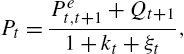
where kt![]() represents the so-called user cost of housing and ξt
represents the so-called user cost of housing and ξt![]() can be interpreted as the risk premium for buying over renting a house. In particular, the user cost kt
can be interpreted as the risk premium for buying over renting a house. In particular, the user cost kt![]() includes the risk-free interest rate (or mortgage rate), denoted as rt
includes the risk-free interest rate (or mortgage rate), denoted as rt![]() , as well as other costs, such as depreciation and maintenance costs, property tax, etc. (see, e.g. Himmelberg et al., 2005). As shown in Bolt et al. (2014) and Dieci and Westerhoff (2016), Eq. (33) is consistent with the assumptions of mean-variance demand and market clearing in the housing market.
, as well as other costs, such as depreciation and maintenance costs, property tax, etc. (see, e.g. Himmelberg et al., 2005). As shown in Bolt et al. (2014) and Dieci and Westerhoff (2016), Eq. (33) is consistent with the assumptions of mean-variance demand and market clearing in the housing market.
5.1.1 Heterogeneous Expectations, Fundamentals, and Temporary Bubbles
In this section we discuss the model of Bolt et al. (2014). They address the issue of house price bubbles and crashes, disconnected from the dynamics of the rent and fundamental price, in a model of the housing market with behavioral heterogeneity and evolutionary selection of beliefs. Following Boswijk et al. (2007), the rent Qt![]() in (33) follows an exogenous process, namely, a geometric Brownian motion with drift, Qt+1=(1+g)ϵtQt
in (33) follows an exogenous process, namely, a geometric Brownian motion with drift, Qt+1=(1+g)ϵtQt![]() , where {ϵt}
, where {ϵt}![]() are i.i.d. log-normal, with unit conditional mean. The user cost kt
are i.i.d. log-normal, with unit conditional mean. The user cost kt![]() (here reduced to the interest rate for simplicity) and the risk premium ξt
(here reduced to the interest rate for simplicity) and the risk premium ξt![]() in (33) are assumed constant kt=rt=r
in (33) are assumed constant kt=rt=r![]() , ξt=ξ
, ξt=ξ![]() , with r+ξ>g
, with r+ξ>g![]() .27 In the reference case of homogeneous and correct expectations, a benchmark ‘fundamental’ solution P⁎t
.27 In the reference case of homogeneous and correct expectations, a benchmark ‘fundamental’ solution P⁎t![]() can be obtained from Eq. (33), namely, P⁎t=Et[∑∞s=1Qt+s(1+r+ξ)−s]=Qt+1[∑∞s=1(1+g)s−1(1+r+ξ)−s]=Qt+1/(r+ξ−g)
can be obtained from Eq. (33), namely, P⁎t=Et[∑∞s=1Qt+s(1+r+ξ)−s]=Qt+1[∑∞s=1(1+g)s−1(1+r+ξ)−s]=Qt+1/(r+ξ−g)![]() .
.
Heterogeneity in expectations is captured by the interplay of regressive (fundamentalist) and extrapolative (chartist) beliefs (indexed by h∈{f,c}![]() , respectively), with time-varying proportions nc,t
, respectively), with time-varying proportions nc,t![]() and nf,t=1−nc,t
and nf,t=1−nc,t![]() . More precisely, investors form their beliefs about the relative deviation between the price and the fundamental in the next period, Xt+1:=
. More precisely, investors form their beliefs about the relative deviation between the price and the fundamental in the next period, Xt+1:=![]() (Pt+1−P⁎t+1)/P⁎t+1
(Pt+1−P⁎t+1)/P⁎t+1![]() , according to the linear rules Eh,t(Xt+1)=ϕhXt−1
, according to the linear rules Eh,t(Xt+1)=ϕhXt−1![]() , h∈{f,c}
, h∈{f,c}![]() , where ϕf<1
, where ϕf<1![]() and ϕc>1
and ϕc>1![]() characterize regressive and extrapolative beliefs, respectively. As a consequence,28 asset pricing Eq. (33) takes the following recursive form in relative deviations from the fundamental price, given proportions nc,t
characterize regressive and extrapolative beliefs, respectively. As a consequence,28 asset pricing Eq. (33) takes the following recursive form in relative deviations from the fundamental price, given proportions nc,t![]() and
and ![]() :
:
(34)
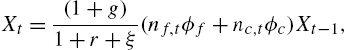
where ![]() is the average market expectation of
is the average market expectation of ![]() . It is also clear from (34) that the direction of the price change is remarkably affected by the current belief distribution. Strategies' proportions are determined by a logistic switching model with a-synchronous updating (see, e.g. Diks and van der Weide, 2005), according to
. It is also clear from (34) that the direction of the price change is remarkably affected by the current belief distribution. Strategies' proportions are determined by a logistic switching model with a-synchronous updating (see, e.g. Diks and van der Weide, 2005), according to ![]() , where
, where ![]() and
and ![]() are fitness measures for chartists and fundamentalists, based on the realized excess profits in the previous period.29 The model is described by a high-dimensional nonlinear dynamical system.
are fitness measures for chartists and fundamentalists, based on the realized excess profits in the previous period.29 The model is described by a high-dimensional nonlinear dynamical system.
Based on earlier literature and on quarterly data on house price and rent indices from OECD databases, Bolt et al. (2014) calibrate the fundamental model parameters and obtain the price-fundamental deviations ![]() for each of eight different countries (US, UK, NL, JP, CH, ES, SE, and BE).30 In a second step, the behavioral parameters of the agent-based model are estimated based on the time series
for each of eight different countries (US, UK, NL, JP, CH, ES, SE, and BE).30 In a second step, the behavioral parameters of the agent-based model are estimated based on the time series ![]() (with the fundamental parameters fixed during the estimation). Since the model is governed by a nonlinear time-varying AR(1) process, once white noise is added to Eq. (34), it can be estimated by nonlinear least squares. In particular, among the estimated behavioral parameters,
(with the fundamental parameters fixed during the estimation). Since the model is governed by a nonlinear time-varying AR(1) process, once white noise is added to Eq. (34), it can be estimated by nonlinear least squares. In particular, among the estimated behavioral parameters, ![]() is significantly larger than 1 (chartists expect that the bubble will continue in the near future) and the difference
is significantly larger than 1 (chartists expect that the bubble will continue in the near future) and the difference ![]() is significant for all countries. This confirms the destabilizing impact of extrapolators and the presence of time-varying heterogeneity in the way agents form expectations. For all countries, long-lasting temporary house price bubbles are identified, driven or amplified by extrapolation (in particular, US, UK, NL SE, and ES display strong housing bubbles over the period 2004–2007). When these bubbles burst, the correction of housing prices is reinforced by investors' switching to a mean-reverting fundamental strategy. Remarkably, for all countries, the estimated parameters are close to regimes of multiple equilibria and/or global instability of the underlying nonlinear switching model. This fact has important policy implications, as the control of certain parameters may prevent the system from getting too close to bifurcation. For instance, the (mortgage) interest rate turns out to be one of the parameters that may shift the nonlinear system closer to multiple equilibria and global instability, whenever it becomes too low. The paper also shows that the qualitative in-sample and out-of-sample predictions of the non-linear switching model differ considerably from those of standard linear benchmark models with a rational representative agent, which is also important from a policy viewpoint.
is significant for all countries. This confirms the destabilizing impact of extrapolators and the presence of time-varying heterogeneity in the way agents form expectations. For all countries, long-lasting temporary house price bubbles are identified, driven or amplified by extrapolation (in particular, US, UK, NL SE, and ES display strong housing bubbles over the period 2004–2007). When these bubbles burst, the correction of housing prices is reinforced by investors' switching to a mean-reverting fundamental strategy. Remarkably, for all countries, the estimated parameters are close to regimes of multiple equilibria and/or global instability of the underlying nonlinear switching model. This fact has important policy implications, as the control of certain parameters may prevent the system from getting too close to bifurcation. For instance, the (mortgage) interest rate turns out to be one of the parameters that may shift the nonlinear system closer to multiple equilibria and global instability, whenever it becomes too low. The paper also shows that the qualitative in-sample and out-of-sample predictions of the non-linear switching model differ considerably from those of standard linear benchmark models with a rational representative agent, which is also important from a policy viewpoint.
5.1.2 Heterogeneous Beliefs, Boom-Bust Cycles, and Supply Conditions
In a similar two-beliefs asset pricing framework for housing markets, Dieci and Westerhoff, 2016 investigate how expectations-driven house price fluctuations interact with supply conditions (namely, housing supply elasticity and the existing stock of housing). For this purpose, an evolving mix of extrapolative and regressive beliefs is nested into a traditional stock-flow housing market framework (DiPasquale and Wheaton, 1992, Poterba, 1984) that connects the house price to the rent level and housing stock. Although the house price is still determined by a temporary equilibrium condition formally similar to (33), the model has a number of peculiar features. First, the (constant) user cost ![]() now includes also the depreciation rate d, namely,
now includes also the depreciation rate d, namely, ![]() . Second, the rent paid in period
. Second, the rent paid in period ![]() ,
, ![]() , is determined endogenously and, ceteris paribus, negatively related to the current stock of housing
, is determined endogenously and, ceteris paribus, negatively related to the current stock of housing ![]() , namely,
, namely, ![]() , with
, with ![]() . This is due to market clearing for rental housing, where supply of housing services is assumed to be proportional to the stock of housing while demand is a downward-sloping function of the rent. Third, the stock of housing evolves due to depreciation and new constructions, where the latter depends positively on the observed price level:
. This is due to market clearing for rental housing, where supply of housing services is assumed to be proportional to the stock of housing while demand is a downward-sloping function of the rent. Third, the stock of housing evolves due to depreciation and new constructions, where the latter depends positively on the observed price level:
(35)
In each period, investment demand for housing based on standard mean-variance optimization (see, e.g. Brock and Hommes, 1998) results in the following market clearing condition31:
(36)
where ![]() is the average market expectation (across investors) and parameter
is the average market expectation (across investors) and parameter ![]() is directly related to investors' risk aversion and second moment beliefs, assumed to be constant and identical across investors. The left-hand side of (36) represents the average individual demand (desired holdings of housing stock) and is proportional to the expected excess profit on one housing unit, taking both rental earnings and depreciation into account. Note that a larger stock
is directly related to investors' risk aversion and second moment beliefs, assumed to be constant and identical across investors. The left-hand side of (36) represents the average individual demand (desired holdings of housing stock) and is proportional to the expected excess profit on one housing unit, taking both rental earnings and depreciation into account. Note that a larger stock ![]() and/or a larger risk perception α require a larger expected excess profit in order for the market to clear, which results in a lower market clearing price, ceteris paribus. By defining the ‘risk-adjusted’ rent
and/or a larger risk perception α require a larger expected excess profit in order for the market to clear, which results in a lower market clearing price, ceteris paribus. By defining the ‘risk-adjusted’ rent ![]() , one obtains the following house pricing equation32:
, one obtains the following house pricing equation32:
(37)

Dynamical system (37) and (35) admits a unique steady state, implicitly defined by ![]() and
and ![]() , which can be regarded as the fundamental steady state (FSS), where the fundamental price
, which can be regarded as the fundamental steady state (FSS), where the fundamental price ![]() obeys to a standard ‘discounted dividend’ representation. Consistently, the price-rent ratio at the FSS can be expressed as the reciprocal of the user cost (including the required housing risk premium):
obeys to a standard ‘discounted dividend’ representation. Consistently, the price-rent ratio at the FSS can be expressed as the reciprocal of the user cost (including the required housing risk premium):
(38)
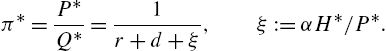
Although the model admits the same FSS under a wide spectrum of expectations schemes, investors' beliefs may remarkably affect the nature of the dynamical system, the way it reacts to shocks, and how it behaves sufficiently far from the FSS. In the reference case of perfect foresight, with homogeneous price expectation satisfying ![]()
![]() , the FSS is saddle-path stable. In the presence of a ‘fundamental’ shock (e.g., an unanticipated and permanent interest rate reduction) shifting the FSS in the plane
, the FSS is saddle-path stable. In the presence of a ‘fundamental’ shock (e.g., an unanticipated and permanent interest rate reduction) shifting the FSS in the plane ![]() , the adjustment process towards the new FSS implies an initial price overshooting followed by a monotonic decline toward the new equilibrium price
, the adjustment process towards the new FSS implies an initial price overshooting followed by a monotonic decline toward the new equilibrium price ![]() , whereas the stock adjusts to level
, whereas the stock adjusts to level ![]() gradually, without overbuilding, as shown in Fig. 11. This dynamic pattern is due to the assumed full rationality of housing market investors, by which the system can jump to the new saddle path immediately after the shock. Remarkably, the qualitative pattern illustrated Fig. 11 is extremely robust to changes of the parameters (in particular, it is unaffected by the response of housing supply).
gradually, without overbuilding, as shown in Fig. 11. This dynamic pattern is due to the assumed full rationality of housing market investors, by which the system can jump to the new saddle path immediately after the shock. Remarkably, the qualitative pattern illustrated Fig. 11 is extremely robust to changes of the parameters (in particular, it is unaffected by the response of housing supply).
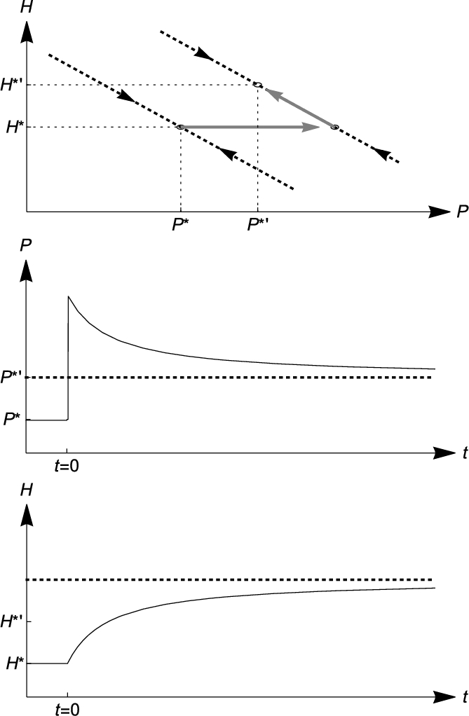
In contrast, by assuming backward-looking and heterogeneous expectations, the stability properties of the FSS and the nature of price and stock fluctuations depend on the way investors' beliefs coevolve with the housing market itself. The average price expectation is specified as
(39)
where ![]() and
and ![]() ,
, ![]() , represent the extrapolative and regressive components, respectively. Similar to (32), the market weight of extrapolative and regressive beliefs evolves endogenously, depending on market circumstances. The market proportion of extrapolators is specified as
, represent the extrapolative and regressive components, respectively. Similar to (32), the market weight of extrapolative and regressive beliefs evolves endogenously, depending on market circumstances. The market proportion of extrapolators is specified as ![]() , where
, where ![]() , is a ‘bell-shaped’ function of the observed mispricing, governed by a (possibly state-dependent) sensitivity coefficient
, is a ‘bell-shaped’ function of the observed mispricing, governed by a (possibly state-dependent) sensitivity coefficient ![]() .33
.33
The rent and the supply of new constructions are modeled as isoelastic functions, namely, ![]() ,
, ![]() ,
, ![]() . Dynamical system (37) and (35) has a locally stable FSS34 only for sufficiently weak extrapolation (low parameter γ). For large enough γ, the model predicts that an initial positive deviation from the fundamental price tends to be amplified by investors' behavior. However, the stability loss generated by strong extrapolation may result in different scenarios, depending on the elasticity of housing supply, μ. Under a relatively inelastic housing supply, the extrapolation generates two additional (locally stable) non-fundamental steady states (NFSS), via a so-called pitchfork bifurcation. Such ‘bubble equilibria’ are characterized by higher (respectively lower) levels of the price-rent ratio than the fundamental price-rent ratio
. Dynamical system (37) and (35) has a locally stable FSS34 only for sufficiently weak extrapolation (low parameter γ). For large enough γ, the model predicts that an initial positive deviation from the fundamental price tends to be amplified by investors' behavior. However, the stability loss generated by strong extrapolation may result in different scenarios, depending on the elasticity of housing supply, μ. Under a relatively inelastic housing supply, the extrapolation generates two additional (locally stable) non-fundamental steady states (NFSS), via a so-called pitchfork bifurcation. Such ‘bubble equilibria’ are characterized by higher (respectively lower) levels of the price-rent ratio than the fundamental price-rent ratio ![]() in Eq. (38). Therefore, under a weak supply response, a positive mispricing at time
in Eq. (38). Therefore, under a weak supply response, a positive mispricing at time ![]() results in a long-lasting price bubble and overbuilding, in the absence of exogenous shocks (the top left panel of Fig. 12). Things are quite different under a more elastic housing supply. Although the initial price path is very similar, a prompt supply response results in a larger growth of the housing stock, which causes a price decline and, ultimately, the endogenous bursting of the bubble (the top right panel). This second scenario is associated with a stable closed orbit, generated via a Neimark–Sacker bifurcation. The larger the supply response, the larger and faster the growth of the stock, the shorter the bubble period (the bottom panels of Fig. 12).
results in a long-lasting price bubble and overbuilding, in the absence of exogenous shocks (the top left panel of Fig. 12). Things are quite different under a more elastic housing supply. Although the initial price path is very similar, a prompt supply response results in a larger growth of the housing stock, which causes a price decline and, ultimately, the endogenous bursting of the bubble (the top right panel). This second scenario is associated with a stable closed orbit, generated via a Neimark–Sacker bifurcation. The larger the supply response, the larger and faster the growth of the stock, the shorter the bubble period (the bottom panels of Fig. 12).

Fig. 13 illustrates a further scenario in which supply elasticity may affect bubbles in a similar manner. The top-left panel is a phase-space representation in the plane of house price and stock (in relative deviations from ![]() and
and ![]() , respectively) of the dynamics depicted in the top-left panel in Fig. 12. The underlying regime has three equilibria, two of which are visible in Fig. 13, namely, the FSS and the ‘upper’ NFSS. The light and dark gray regions represent the basins of attraction of the coexisting NFSS, whereas the (saddle) FSS lies on the boundary of the basins. The top panels and the bottom-left panel indicate that, the larger the supply elasticity, the closer the NFSS gets to the boundary of its basin. The bubble equilibrium thus becomes less and less robust to exogenous noise, although it continues to be locally stable. In particular, its basin of attraction may become very small (white area in the bottom-right panel of Fig. 13).35 From the viewpoint of nonlinear dynamics, the phenomena illustrated in Fig. 13 are global, in the sense that they are independent of the local stability properties of the coexisting steady states.
, respectively) of the dynamics depicted in the top-left panel in Fig. 12. The underlying regime has three equilibria, two of which are visible in Fig. 13, namely, the FSS and the ‘upper’ NFSS. The light and dark gray regions represent the basins of attraction of the coexisting NFSS, whereas the (saddle) FSS lies on the boundary of the basins. The top panels and the bottom-left panel indicate that, the larger the supply elasticity, the closer the NFSS gets to the boundary of its basin. The bubble equilibrium thus becomes less and less robust to exogenous noise, although it continues to be locally stable. In particular, its basin of attraction may become very small (white area in the bottom-right panel of Fig. 13).35 From the viewpoint of nonlinear dynamics, the phenomena illustrated in Fig. 13 are global, in the sense that they are independent of the local stability properties of the coexisting steady states.
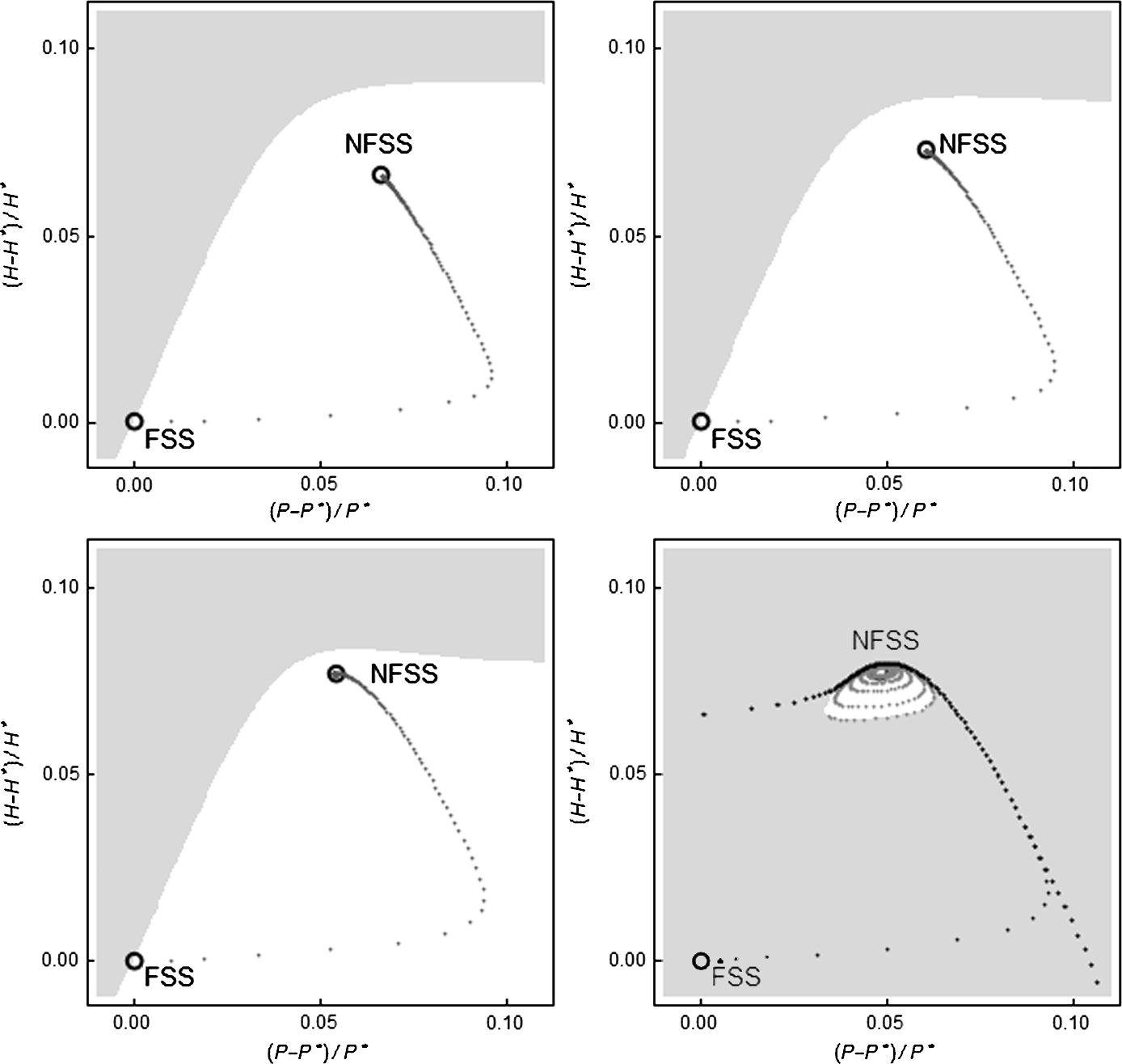
The qualitative results produced by this model are in agreement with recent research on housing market bubbles and urban economics, reporting that a more elastic housing supply is associated to shorter bubbles, smaller price increases and larger stock adjustments (see, e.g. Glaeser et al., 2008).36 This model thus provides a ‘nonlinear economic dynamics’ interpretation on the observed role of supply elasticity in shaping housing bubbles and crashes, based on bifurcation analysis and on a simple HAM framework.
5.2 Disequilibrium Price Adjustments
Further HAMs of the housing market depart from equilibrium asset pricing equation (33) and rest on the view that prices adjust to excess demand in each period in disequilibrium. This may lead to different dynamics from that observed under market clearing. However, the phenomena reported in the previous section appear to be quite robust to such alternative specifications. In particular, Dieci and Westerhoff (2012) consider the following linear price adjustment equation
(40)
Housing stock ![]() evolves similarly to (35), namely,
evolves similarly to (35), namely, ![]() ,
, ![]() . The housing demand
. The housing demand ![]() (interpreted as the desired stock of housing) is made up of ‘real demand’
(interpreted as the desired stock of housing) is made up of ‘real demand’ ![]() (from consumers of housing services) and speculative demand
(from consumers of housing services) and speculative demand ![]() (from investors motivated by short-term capital gains). The two demand components are modeled, respectively, as follows:
(from investors motivated by short-term capital gains). The two demand components are modeled, respectively, as follows:
(41)
(42)
where ![]() and
and ![]() are chartist and fundamentalist demand, respectively. Again, the proportion of extrapolators
are chartist and fundamentalist demand, respectively. Again, the proportion of extrapolators ![]() evolves according to weighting function
evolves according to weighting function ![]() introduced in Section 5.1.2. In particular, while real demand
introduced in Section 5.1.2. In particular, while real demand ![]() depends linearly and negatively on the current price level, speculative demand
depends linearly and negatively on the current price level, speculative demand ![]() results in a nonlinear, cubic-like function of
results in a nonlinear, cubic-like function of ![]() .37 In (42),
.37 In (42), ![]() is the FSS, corresponding to the unique steady state of the baseline case without speculative demand, namely,
is the FSS, corresponding to the unique steady state of the baseline case without speculative demand, namely, ![]() ,
, ![]() . Using the change of variables
. Using the change of variables ![]() ,
, ![]() , one obtains the following two-dimensional nonlinear system in deviations from the FSS:
, one obtains the following two-dimensional nonlinear system in deviations from the FSS:

The analytical and numerical study of the dynamical system delivers clear-cut results about the emergence of housing bubbles and crashes and the joint role played by chartist demand parameter, ![]() , and the slopes of ‘real’ demand and supply schedules, b and m. In particular, similar to Dieci and Westerhoff (2016), parameter
, and the slopes of ‘real’ demand and supply schedules, b and m. In particular, similar to Dieci and Westerhoff (2016), parameter ![]() may destabilize the steady state via a pitchfork bifurcation, if the housing supply curve is sufficiently flat (low m), or via a Neimark–Sacker bifurcation, if the supply schedule is sufficiently sloped (large m). Moreover, in both scenarios, large
may destabilize the steady state via a pitchfork bifurcation, if the housing supply curve is sufficiently flat (low m), or via a Neimark–Sacker bifurcation, if the supply schedule is sufficiently sloped (large m). Moreover, in both scenarios, large ![]() results in a ‘route’ to complexity and endogenous irregular bubbles and crashes. In particular, in the pitchfork scenario, two locally attracting NFSS may evolve into more complex (disjoint) attractors and, ultimately, merge into a unique attractor (through a so-called homoclinic bifurcation). The motion of the system on this attractor is characterized by irregular dynamics in the bull or bear market regions, and by sudden, seemingly unpredictable switching between the bull and bear markets (the top-left panel of Fig. 14) and slow change of the stock level (the top-right panel).38 In the Neimark–Sacker scenario, irregular bubbles of different size and duration, followed by sudden crashes, can be observed (the bottom-left panel), with larger and more frequent stock fluctuations (the bottom-right panel). This kind of motion is also due to a complex attractor, originally born as a regular closed curve via a Neimark–Sacker bifurcation.
results in a ‘route’ to complexity and endogenous irregular bubbles and crashes. In particular, in the pitchfork scenario, two locally attracting NFSS may evolve into more complex (disjoint) attractors and, ultimately, merge into a unique attractor (through a so-called homoclinic bifurcation). The motion of the system on this attractor is characterized by irregular dynamics in the bull or bear market regions, and by sudden, seemingly unpredictable switching between the bull and bear markets (the top-left panel of Fig. 14) and slow change of the stock level (the top-right panel).38 In the Neimark–Sacker scenario, irregular bubbles of different size and duration, followed by sudden crashes, can be observed (the bottom-left panel), with larger and more frequent stock fluctuations (the bottom-right panel). This kind of motion is also due to a complex attractor, originally born as a regular closed curve via a Neimark–Sacker bifurcation.

 ). Bottom panels: house price and stock in the ‘Neimark–Sacker’ scenario (b = 0.05, m = 0.5,
  ). Other parameters are d = 0.02,
  , ν = 1 for all panels.
Kouwenberg and Zwinkels (2015) develop and estimate a housing market model with a structure similar to Dieci and Westerhoff (2012). For estimation purposes, their model is expressed in log price, ![]() , and the log-fundamental
, and the log-fundamental ![]() is modeled as a time-varying reference value. The demand functions from consumers and investors are interpreted as flows (desired transactions) and so is supply (identified with the flow of new constructions). While fundamentalist demand is based on current mispricing, chartist demand is based on the extrapolation of a time average of past returns. The proportions of chartists and fundamentalists evolve endogenously based on past performances (related to past observed forecast errors), according to a standard logit switching model. The model is expressed as:
is modeled as a time-varying reference value. The demand functions from consumers and investors are interpreted as flows (desired transactions) and so is supply (identified with the flow of new constructions). While fundamentalist demand is based on current mispricing, chartist demand is based on the extrapolation of a time average of past returns. The proportions of chartists and fundamentalists evolve endogenously based on past performances (related to past observed forecast errors), according to a standard logit switching model. The model is expressed as:
(43)
where ![]() is the log-return on housing investment,
is the log-return on housing investment, ![]() is a random noise term. The demand and supply are defined as follows:
is a random noise term. The demand and supply are defined as follows:
(44)

Chartist proportion is given by ![]() , where
, where ![]() , and
, and ![]() is a sum of past absolute forecast errors of agents of type h,
is a sum of past absolute forecast errors of agents of type h, ![]() . Similar to Eqs. (41) and (42), the housing demand
. Similar to Eqs. (41) and (42), the housing demand ![]() in (44) includes the consumer demand component and the speculative demand terms due to chartists and fundamentalists, respectively.39
in (44) includes the consumer demand component and the speculative demand terms due to chartists and fundamentalists, respectively.39
The model can be estimated by rewriting it as single non-linear equation and applying maximum likelihood estimation. Estimation results (based on U.S. quarterly time-series data on prices and rents)40 reveal that the coefficients for the fundamentalist and chartist rules are significant and have the expected signs. The positive and significant sign of the estimated intensity of choice parameter (β) implies that agents tend to switch following recent prediction performance. Interestingly, simulation of the deterministic skeleton of the model (with the parameters set equal to the estimated values) shows that the price does not converge to a stable steady state value, but to a stable limit cycle. Hence, an endogenous nonlinear motion appears to be an important part of U.S. housing market dynamics.
A widely reported empirical fact about real estate returns is the presence of short-term positive autocorrelation and long-term mean-reversion (see, e.g. Capozza and Israelsen, 2007, Case and Shiller, 1989, 1990). This fact is, more or less explicitly, part of the motivation for the chartist-fundamentalist framework adopted in the models reviewed in this section. Kouwenberg and Zwinkels (2014) build an econometric model that includes explicitly these two competing components of housing returns. The model is based on a VECM equation, modified to allow for smoothly changing weights of the autoregressive and error correction components, conditional on the value of a transition variable that depends on past relative forecast errors (a so-called smooth transition model). In fact, the econometric model is a particular case of the behavioral model described above (Kouwenberg and Zwinkels, 2015). The analysis shows that house prices are cointegrated with a rent-based estimate of the fundamental value. Estimation results (using quasi-maximum likelihood estimation, based on quarterly US national house price index data) indicate that the strength of the autocorrelation and the long-term mean reversion in housing returns vary significantly over time, depending on recent forecasting performances. The time variation captured by the smooth transition model can produce better out-of-sample forecasts of house price index returns than alternative models.
6 HAMs and Market Microstructure
Limit order markets (LOM) are the most active and dominating financial markets (O'Hara, 2001; Easley et al., 2013; O'Hara, 2015). A core and challenging issue in dynamical LOM models is the endogenous order choice of investors to submit either market or limit orders. It is important to understand how investors trade based on their asymmetric information and what they can learn from order book information. The current literature of limit order market models faces two main challenges. First, they mainly focus on perfectly rational information-based trade and order choice of informed traders. However, within rational expectation equilibrium framework, “a model that incorporates the relevant frictions of limit-order markets (such as discrete prices, staggered trader arrivals, and asymmetric information) does not readily admit a closed-form solution (Goettler et al., 2009)”. This limits the explanatory power of this framework. Second, rational expectation framework simplifies the order choice behavior of uninformed traders by introducing either private value or time preferences exogenously. However, as pointed out by O'Hara (2001), “It is the uninformed traders who provide the liquidity to the informed, and so understanding their behavior can provide substantial insight and intuition into the trading process”. Therefore what uninformed traders can learn from order book information and how learning affects their order choice and the behavior of informed traders are not clear.
Recent development of HAMs and computationally oriented agent-based simulations provide a framework to deal with these challenges in LOM models. With great flexibility in modeling complexity and learning, this framework offers a very promising and integrated approach to the research in market microstructure. Within this framework, many features including asymmetric information, learning, and order choice can be articulated. It can provide an insight into the impact of heterogeneous trading rules on limit order book and order flows (Chiarella and Iori, 2002, Chiarella et al., 2009b, 2012b, Kovaleva and Iori, 2014), interplay of different market architectures and different types of regulatory measures, such as price limits (Yeh and Yang, 2010), transaction taxes (Pellizzari and Westerhoff, 2009), short-sales constraints (Anufriev and Tuinstra, 2013). It also sheds light on the costs and benefits of financial regulations (Lensberg et al., 2015).
This section discusses briefly the recent developments along this line, in particular the contributions of Chiarella et al. (2015a, 2017) and Arifovic et al. (2016). We first focus on how computationally oriented HAMs can be used to replicate the stylized facts in LOM and provide possible mechanism explanation to these stylized facts in Section 6.1. We then discuss how genetic algorithm (GA) learning with a classifier system can help to understand the joint impact of market information, market microstructure mechanisms, and behavioral factors on the dynamics of LOM characterized by information asymmetry and complexity in order flows and trading in Section 6.2. We also examine the impact of high frequency trading (HFT) and learning on information aggregation, market liquidity, and price discovery in Section 6.3, demonstrating that the incentive for high frequency traders not to trade too fast can be consistent with price information efficiency. We also discuss some implications on market design and regulation in Section 6.4.
6.1 Stylized Facts in Limit Order Markets
Agent-based computational finance has made a significant contribution to characterize the stylized facts in financial markets, as discussed in Section 2. As pointed out in Chen et al. (2012) and Gould et al. (2013), after several prototypes have successfully replicated a number of financial stylized facts of the low frequency data, the next milestone is to see whether HAMs can also be used to replicate the features in high frequency domain.
Various stylized facts in limit order markets have been documented in market microstructure literature. According to surveys by Chen et al. (2012) and Gould et al. (2013), apart from the stylized facts in the time series of returns, including fat tails, the absence of autocorrelation in returns, volatility clustering, and long memory in the absolute returns, the limit order market has its own stylized facts. They include long memory in the bid-ask spread and trading volume, hump shapes in order depth profiles of order books, non-linear relationship between trade imbalance and mid-price return, and diagonal effect or event clustering in order submission types, among the most common and important statistical regularities in LOM. They have become the most important criteria to justify the explanatory power of agent-based LOM.
A number of HAMs of market microstructure have been able to replicate some of the stylized facts. They include zero-intelligence models and HAMs (see Chen et al., 2012 and Gould et al., 2013 for surveys). The zero-intelligence models show that some of the stylized facts, such as fat tail and possible volatility and event clusterings, are generated by trading mechanism, instead of agents' strategic behavior. Different from the zero-intelligence models, HAMs consider agents' strategic behaviors as potential explanations to the stylized facts. Chiarella and Iori (2002) argue that substantial heterogeneity must exist between market participants in order for the highly non-trivial properties of volatility to emerge in real limit order markets. By assuming that agents use strategies that blend three components (fundamentalist, chartist, and noisy), Chiarella et al. (2009b) provide a computational HAM of an order-driven market to study order book and flow dynamics. Inspired by the theoretically oriented dynamic analysis of moving average rules in Chiarella et al. (2006b), Chiarella et al. (2012b) conduct a dynamic analysis of a more realistic microstructure model of continuous double auctions. When agents switch between either fundamentalists or chartists based on their relative performance, they show that the model is able to characterize volatility clustering, insignificant autocorrelations (ACs) of returns and significantly slow-decaying ACs of the absolute returns. The result suggests that both behavioral traits and realistic microstructure have a role in explaining several statistical properties of returns.
In a modified version of Chiarella et al. (2009b), Kovaleva and Iori (2014) investigate the interrelation between pre-trade quote transparency and stylized properties of order-driven markets populated by traders with heterogeneous beliefs. The model is able to capture negative skewness of stock returns and volatility clustering once book depth is visible to traders. Their simulation analysis reveals that full quote transparency contributes to convergence in traders' actions, while exogenously partial transparency restriction may exacerbate long-range dependencies. However, replicating most of these stylized facts in LOM simultaneously remains very challenging.
When modeling agents' expectation, behavioral sentiment plays an important role. Barberis et al. (1998) and Daniel et al. (1998) point out that certain well-known psychological biases, including conservatism, representativeness heuristic, overconfidence and biased self-attribution, not only characterize how people actually behave, but can also explain a range of empirical findings, such as underreaction and overreaction of stock prices to news, excess volatility and post-earnings announcement drift. By incorporating behavioral sentiment to a LOM model, Chiarella et al. (2017) show that the behavioral sentiment not only helps to replicate most of the stylized facts simultaneously in LOM, but also plays a unique role in explaining these stylized facts that cannot be explained by noise trading. They include fat tails in the return distribution, long memory in the trading volume, an increasing and non-linear relationship between trading imbalance and mid-price returns, as well as the diagonal effect or event clustering in order submission types.
6.2 Information and Learning in Limit Order Market
Because of information asymmetry and growing complexity in order flows and trading in LOM, the endogenous order choice based on the order book conditions is a core and challenging issue, as highlighted by Rosu (2012). How traders' learning, in particular uninformed traders, from order book information affect their order choice and limit order market becomes important. Recently, Chiarella et al. (2015a) provide a LOM model with adaptive learning through genetic algorithm (GA) with classifier system, trying to explore the joint impact of adaptive learning and information asymmetric on trading behavior, market liquidity, and price discovery.
Since introduced firstly by Holland (1975), GA and classifier system have been used in agent-based models to examine learning and evolution in Santa Fe Institute artificial stock market (SFI-ASM) (Arthur et al., 1997a, LeBaron et al., 1999) and economic models (Marimon et al., 1990, Lettau and Uhlig, 1999, Allen and Carroll, 2001). In LOM, LeBaron and Yamamoto (2008) employ GA to capture the imitation behavior among heterogeneous beliefs. Darley and Outkin (2007) use adaptive learning to evolve trading rules of market makers and apply their simulations to the Nasdaq market in 1998. The adaptive learning has been widely used in financial markets. However most HAMs with adaptive learning and trading are largely driven by the market price instead of asymmetric information, which is the focus of microstructure literature in LOM. This brings a significant difference in the dynamics of LOM.
Unlike informed traders, uninformed traders do not have the information about the current, but lagged fundamental value. By combining information processing of market conditions and order choice into GA with a classifier system, Chiarella et al. (2015a) show that behavior heterogeneity of traders is endogenously emerged from their learning and trading. This approach fills the gap between agent-based computational finance and the mainstream market microstructure since Kyle (1985). They show that, measured by the average usage of different market information, trading rules under the GA learning become stationary and hence effective in the long-run. In particular, the learning of uninformed traders improves market information efficiency, which is not necessarily the case when informed traders learn. The learning also makes uninformed traders submit less aggressive limit orders but more market orders, while it makes informed traders submit less market orders and more aggressive limit orders. In general, both informed and uninformed traders provide liquidity to market at approximately the same rate. The results provide some insight into the effect of learning on order submission behavior, market liquidity and efficiency.
6.3 High Frequency Trading
With technology advance, high frequency trading (HFT) becomes very popular. It also brings a hot debate on the benefit of and market regulation on HFT (O'Hara, 2015). In particular, do financial market participants benefit from HFT and how does HFT affect market efficiency? To examine the effect of HFT and learning in limit order markets, Arifovic et al. (2016) extend the LOM model of Chiarella et al. (2015a) and introduce fast and slow traders with GA learning. Consistent with Grossman and Stiglitz (1980), they show a trade-off between information advantage and profit opportunity for informed HFT. This trade-off leads to a hump-shaped relation between HFT profit, market efficiency, and trading speed. When informed investors trade fast, their information advantage makes HFT more profitable. However, the learning, in particular from uninformed traders, improves information aggregation and efficiency. This then reduces the information advantage of HFT and hence the profit opportunity. HFT in general improves market information efficiency and hence price discovery. However, the trade-off between the information advantage and trading speed of HFT also leads to a hump-shape relation between liquidity consumption and trading speed. HFT improves liquidity consumption and price discovery in general due to information aggregation through the learning. When HFT trade too fast, they submit more market order, which enlarges the spread and reduces market liquidity. This implies that there is an incentive for not trading too fast, which in turn improves price efficiency. The results provide an insight into the profitability of HFT and the current debates and puzzles about the impact of HFT on market liquidity and efficiency.
6.4 HAMs and Microstructure Regulation
Lensberg et al. (2015) build an agent-based framework with market microstructure and delegated portfolio management in order to forecast and compare the equilibrium effects of different regulatory measures: financial transaction tax, short-selling ban and leverage ban. The financial market is characterized by fund managers who trade stocks and bonds in an order-driven market. The process of competition and innovation among different investment styles is modeled through a genetic programming algorithm with tournament selection. However, the heterogeneous trading strategies that emerge from the evolutionary process can be classified by a relatively small number of ‘styles’ (interpreted as value trading, news trading/arbitrage and market making/liquidity supply). The model contributes to understand the pros and cons of different regulations, by providing detailed information on the equilibrium properties of portfolio holdings, order flow, liquidity, cost of capital, price discovery, short-term volatility and long-term price dynamics. By including an exogenous business cycle process, the model also allows to quantify the effects of different regulations during periods of market distress. In particular, it turns out that a financial transaction tax may have a negative impact on liquidity and price discovery, and limited effect on long swings in asset prices.
7 Conclusion and Future Research
This chapter has discussed the latest development of heterogeneous agent models (HAMs) in finance over the last ten years since the publications of the Handbook of Computational Economics in 2006 and, in particular, the Handbook of Financial Markets: Dynamics and Evolution in 2009. It demonstrates a significant contribution of HAMs to finance theory and practice from five broad aspects of financial markets. First of all, inspired by the rich and promising perspectives of the earlier HAMs, we have witnessed a growing supporting evidence on the explanatory power of HAMs to various market anomalies and, in particular, the stylized facts through calibrations and estimations of HAMs to real data in various financial markets over the last decade. More importantly, different from traditional empirical finance and financial econometrics, HAMs provide some insights into economic mechanisms and driving forces of these stylized facts. They therefore lead to some helpful implications in policy and market design. Moreover, the basic framework of earlier HAMs has been naturally developed and extended in two different directions. The first extension to a continuous-time setup provides a unified framework to deal with the effect of historical price information. The framework can be used to examine profitability of fundamental and non-fundamental, such as momentum and contrarian, trading strategies that have been widely used and discussed in financial market practice and finance theory. It also enables to develop optimal asset allocation to incorporate time series momentum and reversal, two of the most important anomalies in financial markets. The second extension to a multiple-risky-asset framework helps to examine the impact of heterogeneous expectations on asset comovements within a financial market, as well as the spill-over effects across markets, and to characterize risk-return relations through an evolutionary CAPM. Moreover, inspired by HAMs of financial markets, a new heterogeneous-agent framework for housing market dynamics has been developed recently. It can well explain house bubbles and crashes, by combining behavioral facts and the real side of housing markets. Finally, the advantage of HAMs in dealing with market complexity plays a unique role in the development of market microstructure modeling. This provides a very promising approach to understand the impact of information, learning, and trading on trading behavior, market liquidity, and price discovery.
The research streams reviewed in this chapter can be developed further in several directions. First, instead of heuristic assumptions on agents' behavioral heterogeneity currently assumed in HAMs, there is a need to provide micro-foundation to endogenize such heuristic heterogeneity among agents. Most of the HAMs investigate the endogenous market mechanism by focusing on the interaction of heterogeneous agents with different expectations (typically fundamentalists and trend followers). Their explanatory power is mainly demonstrated by combining the insights from the nonlinear dynamics of the underlying deterministic model with various noise processes, such as fundamental shocks and noise trading. To a large extent, the HAM literature has not explored the impact of asymmetric information or information uncertainty on agents' behavioral heterogeneity. By considering asymmetric information, which is the focus of traditional finance literature and plays a very important role in financial markets, agents' heterogeneity can be endogenized and micro-founded. This has been illustrated in Section 2.3, based on He and Zheng (2016), by showing how trading heterogeneity can arise endogenously among traders due to uncertainty about the fundamental value information of the risky asset. The development along this line would help to provide economic foundation to the assumed behavioral heterogeneity of agent-based models, which is often critiqued by traditional finance.
Second, as a different aspect of information uncertainty, ambiguity has been introduced in the literature to address various market anomalies and asset pricing (Epstein and Schneider, 2006). More recently, Aliyev and He (2016) discuss the possibilities of capturing efficient market hypothesis and behavioral finance under a general framework based on a broad definition of rationality. They argue that the root of behavioral anomalies comes from the imprecision and reliability of information. A natural combination of heterogeneity and ambiguity would provide a broader framework to financial market modeling and to rationalize market anomalies.
Third, when asset prices are affected by historical price information, we need to develop a portfolio and asset pricing theory in continuous-time to characterize cross-section returns driven by time series momentum in short-run and reversal in long-run. The continuous-time HAMs discussed in Section 3 illustrate the challenging but promising perspectives of this development. Recently, Li and Liu (2016) study the optimal momentum trading strategy when asset prices are affected by historical price information. They provide an optimal way to hedge the momentum crash risk, a newly-found empirical feature, and to significantly improve momentum profits. The techniques developed can potentially be applied to a range of problems in economics and finance, such as momentum, long memory in volatility, post-earnings announcement drift, indexation lags in the inflation-linked bonds.
Fourth, incorporating social interactions and social networks to the current HAMs would be helpful for examining their impact on financial markets and asset pricing. Social interactions are well documented in financial markets, in particular when facing information uncertainty. He et al. (2016a) recently develop a simple evolutionary model of asset pricing and population dynamics to incorporate social interactions among investors with heterogeneous beliefs on information uncertainty. They show that social interactions can lead to mis-pricing and existence of multiple steady state equilibria, generating two different volatility regimes, bi-modal distribution in population dynamics, and stochastic volatility. As pointed out by Hirshleifer (2015), [T]he time has come to move beyond behavioral finance to ‘social finance’. This would provide a fruitful area of research in the near future.
Fifth, HAMS of multiasset markets and financial market interlinkages could be developed further. An interesting research issue is understanding the effect of an increase in the number of risky assets in a setup similar to Chiarella et al. (2013b) and the extent to which standard results on the role of diversification continue to hold in the presence of momentum trading. A related issue concerns the profitability of different trading strategies in a multi-asset framework, their ability to exploit the emerging correlation patterns, and their joint impact on financial market stability. Furthermore, the ability of the evolutionary, heterogeneous-agent CAPM discussed in Section 4.2 to produce a time variation of ex-ante betas has been illustrated through simulation results only. There is a need to have formal statistical tests on the observations based on the numerical simulations. Finally, it would be interesting to see if the time variation of either beta coefficients or risk premia plays a role in explaining the cross section of asset returns.
Sixth, housing market dynamics has only very recently been investigated from the perspective of HAMs. The existing models are mainly aimed at qualitative or quantitative investigations of the role of price extrapolation in generating house price fluctuations. Among the possible interesting developments of this baseline setup is the joint impact of interest rate changes, credit conditions, and investor sentiment on house price fluctuations. In particular, the role of interest rates and credit in triggering house price booms and busts is crucial for policy makers and highly debated in academic literature (see, e.g. Himmelberg et al., 2005 and Jordà et al., 2015). A related issue concerns the dynamic interplay among housing, stock and bond markets, driven by both fundamental shocks, such as interest rate movements, and behavioral factors, such as investors switching to better investment opportunities. Dieci et al. (2017) provide a first attempt in this direction.
Finally, an integrated approach of agent-based models and market microstructure literature would provide a very promising approach, if not the only one, to understand information aggregation, learning, trading, market liquidity and efficiency when facing information asymmetry and growing complexity in market microstructure. This has been illustrated by the discussion in Section 6, but remains largely unexplored.