Chapter 7

Markov Chain Monte Carlo

When a target density f can be evaluated but not easily sampled, the methods from Chapter 6 can be applied to obtain an approximate or exact sample. The primary use of such a sample is to estimate the expectation of a function of X ~ f(x). The Markov chain Monte Carlo (MCMC) methods introduced in this chapter can also be used to generate a draw from a distribution that approximates f, but they are more properly viewed as methods for generating a sample from which expectations of functions of X can reliably be estimated. MCMC methods are distinguished from the simulation techniques in Chapter 6 by their iterative nature and the ease with which they can be customized to very diverse and difficult problems. Viewed as an integration method, MCMC has several advantages over the approaches in Chapter 5: Increasing problem dimensionality usually does not slow convergence or make implementation more complex.

A quick review of discrete-state-space Markov chain theory is provided in Section 1.7. Let the sequence denote a Markov chain for t = 0, 1, 2, . . ., where and the state space is either continuous or discrete. For the types of Markov chains introduced in this chapter, the distribution of X^(t) converges to the limiting stationary distribution of the chain when the chain is irreducible and aperiodic. The MCMC sampling strategy is to construct an irreducible, aperiodic Markov chain for which the stationary distribution equals the target distribution f. For sufficiently large t, a realization X^(t) from this chain will have approximate marginal distribution f. A very popular application of MCMC methods is to facilitate Bayesian inference where f is a Bayesian posterior distribution for parameters X; a short review of Bayesian inference is given in Section 1.5.

The art of MCMC lies in the construction of a suitable chain. A wide variety of algorithms has been proposed. The dilemma lies in how to determine the degree of distributional approximation that is inherent in realizations from the chain as well as estimators derived from these realizations. This question arises because the distribution of X^(t) may differ substantially from f when t is too small (note that t is always limited in computer simulations), and because the X^(t) are serially dependent.

MCMC theory and applications are areas of active research interest. Our emphasis here is on introducing some basic MCMC algorithms that are easy to implement and broadly applicable. In Chapter 8, we address several more sophisticated MCMC techniques. Some comprehensive expositions of MCMC and helpful tutorials include [70, 97, 106, 111, 543, 633]

7.1 Metropolis–Hastings Algorithm

A very general method for constructing a Markov chain is the Metropolis–Hastings algorithm [324, 460]. The method begins at t = 0 with the selection of X⁽⁰⁾ = x⁽⁰⁾ drawn at random from some starting distribution g, with the requirement that . Given X^(t) = x^(t), the algorithm generates X^(t+1) as follows:

1. Sample a candidate value X^∗ from a proposal distribution.

2. Compute the Metropolis–Hastings ratio, where

(7.1)

Note that is always defined, because the proposal X^∗ = x^∗ can only occur if and .

3. Sample a value for X^(t+1) according to the following:

(7.2)

4. Increment t and return to step 1.

We will call the tth iteration the process that generates X^(t) = x^(t). When the proposal distribution is symmetric so that , the method is known as the Metropolis algorithm [460].

Clearly, a chain constructed via the Metropolis–Hastings algorithm is Markov since X^(t+1) is only dependent on X^(t). Whether the chain is irreducible and aperiodic depends on the choice of proposal distribution; the user must check these conditions diligently for any implementation. If this check confirms irreducibility and aperiodicity, then the chain generated by the Metropolis–Hastings algorithm has a unique limiting stationary distribution. This result would seem to follow from Equation (1.44). However, we are now considering both continuous-and discrete-state-space Markov chains. Nevertheless, irreducibility and aperiodicity remain sufficient conditions for convergence of Metropolis–Hastings chains. Additional theory is provided in [462, 543].

To find the unique stationary distribution of an irreducible aperiodic Metropolis–Hastings chain, suppose X^(t) ~ f(x), and consider two points in the state space of the chain, say x₁ and x₂, for which f(x₁) > 0 and f(x₂) > 0. Without loss of generality, label these points in the manner such that .

It follows that the unconditional joint density of X^(t) = x₁ and X^(t+1) = x₂ is , because if X^(t) = x₁ and X^∗ = x₂, then R(x₁, x₂) ≥ 1 so X^(t) = x₂. The unconditional joint density of X^(t) = x₂ and X^(t+1) = x₁ is

(7.3)

because we need to start with X^(t) = x₂, to propose X^∗ = x₁, and then to set X^(t+1) equal to X^∗ with probability R(x₁, x₂). Note that (7.3) reduces to , which matches the joint density of X^(t) = x₁ and X^(t+1) = x₂. Therefore the joint distribution of X^(t) and X^(t+1) is symmetric. Hence X^(t) and X^(t+1) have the same marginal distributions. Thus the marginal distribution of X^(t+1) is f, and f must be the stationary distribution of the chain.

Recall from Equation (1.46) that we can approximate the expectation of a function of a random variable by averaging realizations from the stationary distribution of a Metropolis–Hastings chain. The distribution of realizations from the Metropolis–Hastings chain approximates the stationary distribution of the chain as t progresses; therefore . Some of the useful quantities that can be estimated this way include means , variances , and tail probabilities for constant q, where 1_{A} = 1 if A is true and 0 otherwise. Using the density estimation methods of Chapter 10, estimates of f itself can also be obtained. Due to the limiting properties of the Markov chain, estimates of all these quantities based on sample averages are strongly consistent. Note that the sequence x⁽⁰⁾, x⁽¹⁾, . . . will likely include multiple copies of some points in the state space. This occurs when X^(t+1) retains the previous value x^(t) rather than jumping to the proposed value x^∗. It is important to include these copies in the chain and in any sample averages since the frequencies of sampled points are used to correct for the fact that the proposal density differs from the target density.

In some applications persistent dependence of the chain on its starting value can seriously degrade its performance. Therefore it may be sensible to omit some of the initial realizations of the chain when computing a sample average. This is called the burn-in period and is an essential component of MCMC applications. As with optimization algorithms, it is also a good idea to run MCMC procedures like the Metropolis–Hastings algorithm from multiple starting points to check for consistent results. See Section 7.3 for implementation advice about burn-in, number of chains, starting values, and other aspects of MCMC implementation.

Specific features of good proposal distributions can greatly enhance the performance of the Metropolis–Hastings algorithm. A well-chosen proposal distribution produces candidate values that cover the support of the stationary distribution in a reasonable number of iterations and, similarly, produces candidate values that are not accepted or rejected too frequently [111]. Both of these factors are related to the spread of the proposal distribution. If the proposal distribution is too diffuse relative to the target distribution, the candidate values will be rejected frequently and thus the chain will require many iterations to adequately explore the space of the target distribution. If the proposal distribution is too focused (e.g., has too small a variance), then the chain will remain in one small region of the target distribution for many iterations while other regions of the target distribution will not be adequately explored. Thus a proposal distribution whose spread is either too small or too large can produce a chain that requires many iterations to adequately sample the regions supported by the target distribution. Section 7.3.1 further discusses this and related issues.

Below we introduce several Metropolis–Hastings variants obtained by using different classes of proposal distributions.

7.1.1 Independence Chains

Suppose that the proposal distribution for the Metropolis–Hastings algorithm is chosen such that for some fixed density g. This yields an independence chain, where each candidate value is drawn independently of the past. In this case, the Metropolis–Hastings ratio is

(7.4)

The resulting Markov chain is irreducible and aperiodic if whenever .

Notice that the Metropolis–Hastings ratio in (7.4) can be reexpressed as the ratio of importance ratios (see Section 6.4.1) where f is the target and g is the envelope: If and , then . This reexpression indicates that when is much larger than typical values, then the chain will tend to get stuck for long periods at the current value. Therefore, the criteria discussed in Section 6.3.1 for choosing importance sampling envelopes are also relevant here for choosing proposal distributions: The proposal distribution g should resemble the target distribution f, but should cover f in the tails.

Example 7.1 (Bayesian Inference) MCMC methods like the Metropolis–Hastings algorithm are particularly popular tools for Bayesian inference, where some data y are observed with likelihood function L(θ|y) for parameters θ which have prior distribution p(θ). Bayesian inference is based on the posterior distribution p(θ|y) = c p(θ)L(θ|y), where c is an unknown constant. The difficulty of computing c and other features of the posterior prevents most direct inferential strategies. However, if we can obtain a sample from a Markov chain whose stationary distribution is the target posterior, this sample may be used to estimate posterior moments, tail probabilities, and many other useful quantities, including the posterior density itself. MCMC methods typically allow easy generation of such a sample in the Bayesian context.

A very simple strategy is to use the prior as a proposal distribution in an independence chain. In our Metropolis–Hastings notation, f(θ) = p(θ|y) and g(θ^∗) = p(θ^∗). Conveniently, this means

(7.5)

In other words, we propose from the prior, and the Metropolis–Hastings ratio equals the likelihood ratio. By definition, the support of the prior covers the support of the target posterior, so the stationary distribution of this chain is the desired posterior. There are more specialized MCMC algorithms to sample various types of posteriors in more efficient manners, but this is perhaps the simplest generic approach.

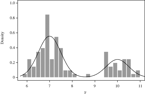
Example 7.2 (Mixture Distribution) Suppose we have observed data y₁, y₂, . . ., y₁₀₀ sampled independently and identically distributed from the mixture distribution

(7.6)

Figure 7.1 shows a histogram of the data, which are available from the website for this book. Mixture densities are common in real-life applications where, for example, the data may come from more than one population. We will use MCMC techniques to construct a chain whose stationary distribution equals the posterior density of δ assuming a Unif(0,1) prior distribution for δ. The data were generated with δ = 0.7, so we should find that the posterior density is concentrated in this area.

Figure 7.1 Histogram of 100 observations simulated from the mixture distribution (7.6) in Example 7.2.

In this example, we try two different independence chains. In the first case we use a Beta(1,1) density as the proposal density, and in the second case we use a Beta(2,10) density. The first proposal distribution is equivalent to a Unif(0,1) distribution, while the second is skewed right with mean approximately equal to 0.167. In this second case values of δ near 0.7 are unlikely to be generated from the proposal distribution.

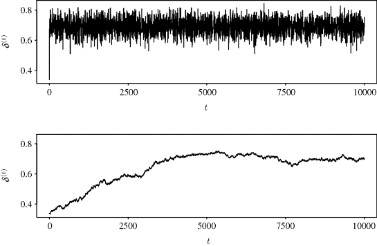
Figure 7.2 shows the sample paths for 10,000 iterations of both chains. A sample path is a plot of the chain realizations δ^(t) against the iteration number t. This plot is useful for investigating the behavior of the Markov chain and is discussed further in Section 7.3.1. The top panel of Figure 7.2 corresponds to the chain generated using the Beta(1,1) proposal density. This panel shows a Markov chain that moves quickly away from its starting value and seems easily able to sample values from all portions of the parameter space supported by the posterior for δ. Such behavior is called good mixing. The lower panel corresponds to the chain using a Beta(2,10) proposal density. The resulting chain moves slowly from its starting value and does a poor job of exploring the region of posterior support (i.e., poor mixing). This chain has clearly not converged to its stationary distribution since drift is still apparent. Of course, the long-run behavior of the chain will in principle allow estimation of aspects of the posterior distribution for δ since the posterior is still the limiting distribution of the chain. Yet, chain behavior like that shown in the bottom panel of Figure 7.2 does not inspire confidence: The chain seems nonstationary, only a few unique values of δ^(t) were accepted, and the starting value does not appear to have washed out. A plot like the lower plot in Figure 7.2 should make the MCMC user reconsider the proposal density and other aspects of the MCMC implementation.

Figure 7.2 Sample paths for δ from independence chains with proposal densities Beta(1,1) (top) and Beta(2,10) (bottom) considered in Example 7.2.

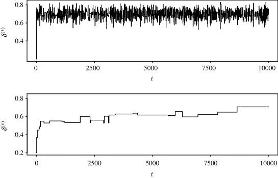
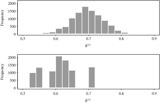
Figure 7.3 shows histograms of the realizations from the chains, after the first 200 iterations have been omitted to reduce the effect of the starting value (see the discussion of burn-in periods in Section 7.3.1.2). The top and bottom panels again correspond to the Beta(1,1) and Beta(2,10) proposal distributions, respectively. This plot shows that the chain with the Beta(1,1) proposal density produced a sample for δ whose mean well approximates the true value (and posterior mean) of δ = 0.7. On the other hand, the chain with the Beta(2,10) proposal density would not yield reliable estimates for the posterior or the true value of δ based on the first 10,000 iterations.

Figure 7.3 Histograms of δ^(t) for iterations 201–10,000 of independence chains with proposal densities Beta(1,1) (top) and Beta(2,10) (bottom) considered in Example 7.2.

7.1.2 Random Walk Chains

A random walk chain is another type of Markov chain produced via a simple variant of the Metropolis–Hastings algorithm. Let X^∗ be generated by drawing ~ h() for some density h and then setting X^∗ = x^(t) + . This yields a random walk chain. In this case, . Common choices for h include a uniform distribution over a ball centered at the origin, a scaled standard normal distribution, and a scaled Student's t distribution. If the support region of f is connected and h is positive in a neighborhood of 0, the resulting chain is irreducible and aperiodic [543].

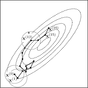
Figure 7.4 illustrates how a random walk chain might progress in a two-dimensional problem. The figure shows a contour plot of a two-dimensional target distribution (dotted lines) along with the first steps of a random walk MCMC procedure. The sample path is shown by the solid line connecting successive values in the chain (dots). The chain starts at x⁽⁰⁾. The second candidate value is accepted to yield x⁽¹⁾. The circles around x⁽⁰⁾ and x⁽¹⁾ show the proposal densities, where h is a uniform distribution over a disk centered at the origin. In a random walk chain, the proposal density at iteration t + 1 is centered around x^(t). Some candidate values are rejected. For example, the 13th candidate value, denoted by , is not accepted, so x⁽¹³⁾ = x⁽¹²⁾. Note how the chain frequently moves up the contours of the target distribution, while also allowing some downhill moves. The move from x⁽¹⁵⁾ to x⁽¹⁶⁾ is one instance where the chain moves downhill.

Figure 7.4 Hypothetical random walk chain for sampling a two-dimensional target distribution (dotted contours) using proposed increments sampled uniformly from a disk centered at the current value. See text for details.

Example 7.3 (Mixture Distribution, Continued) As a continuation of Example 7.2, consider using a random walk chain to learn about the posterior for δ under a Unif(0,1) prior. Suppose we generate proposals by adding a Unif(− a, a) random increment to the current δ^(t). Clearly it is likely that some proposals will be generated outside the interval [0, 1] during the progression of the chain. An inelegant approach is to note that the posterior is zero for any , thereby forbidding steps to such points. An approach that usually is better involves reparameterizing the problem. Let U = logit{δ} = log {δ/(1 − δ)}. We may now run a random walk chain on U, generating a proposal by adding, say, a Unif(− b, b) random increment to u^(t).

There are two ways to view the reparameterization. First, we may run the chain in δ-space. In this case, the proposal density g(· |u^(t)) must be transformed into a proposal density in δ-space, taking account of the Jacobian. The Metropolis–Hastings ratio for a proposed value δ^∗ is then

(7.7)

where, for example, |J(δ^(t))| is the absolute value of the (determinant of the) Jacobian for the transformation from δ to u, evaluated at δ^(t). The second option is to run the chain in u-space. In this case, the target density for δ must be transformed into a density for u, where δ = logit⁻¹{U} = exp {U}/(1 + exp {U}). For U^∗ = u^∗, this yields the Metropolis–Hasting ratio

(7.8)

Since |J(u^∗)| = 1/|J(δ^∗)|, we can see that these two viewpoints produce equivalent chains. Examples 7.10 and 8.1 demonstrate the change-of-variables method within the Metropolis–Hastings algorithm.

The random walk chain run with uniform increments in a reparameterized space may have quite different properties than one generated from uniform increments in the original space. Reparameterization is a useful approach to improving the performance of MCMC methods and is discussed further in Section 7.3.1.4.

Figure 7.5 shows sample paths for δ from two random walk chains run in u-space. The top panel corresponds to a chain generated by drawing ~ Unif(−1,1), setting U^∗ = u^(t) + , and then using (7.8) to compute the Metropolis–Hastings ratio. The top panel in Figure 7.5 shows a Markov chain that moves quickly away from its starting value and seems easily able to sample values from all portions of the parameter space supported by the posterior for δ. The lower panel corresponds to the chain using ~ Unif(−0.01,0.01), which yields very poor mixing. The resulting chain moves slowly from its starting value and takes very small steps in δ-space at each iteration.

Figure 7.5 Sample paths for δ from random walk chains in Example 7.3, run in u-space with b = 1 (top) and b = 0.01 (bottom).

7.2 Gibbs Sampling

Thus far we have treated X^(t) with little regard to its dimensionality. The Gibbs sampler is specifically adapted for multidimensional target distributions. The goal is to construct a Markov chain whose stationary distribution—or some marginalization thereof—equals the target distribution f. The Gibbs sampler does this by sequentially sampling from univariate conditional distributions, which are often available in closed form.

7.2.1 Basic Gibbs Sampler

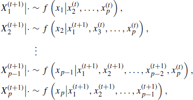
Recall , and denote . Suppose that the univariate conditional density of , denoted , is easily sampled for i = 1, . . ., p. A general Gibbs sampling procedure can be described as follows:

The completion of step 2 for all components of X is called a cycle. Several methods for improving and generalizing the basic Gibbs sampler are discussed in Sections 7.2.3 –7.2.6. In subsequent discussion of the Gibbs sampler, we frequently refer to the term , which represents all the components of x, except for x_i, at their current values, so

Example 7.4 (Stream Ecology) Stream insects called benthic invertebrates are an effective indicator for monitoring stream ecology because their relatively stationary substrate habitation provides constant exposure to contamination and easy sampling of large numbers of individuals. Imagine that at many sites along a stream, insects are collected and classified into several categories based on some ecologically significant criterion. At a particular site, let Y₁, . . ., Y_c denote the counts of insects in each of c different classes.

The probability that an insect is classified in each category varies randomly from site to site, as does the total number collected at each site. For a given site, let P₁, . . ., P_c denote the class probabilities, and let N denote the random total number of insects collected. Suppose, further, that the P₁, . . ., P_c depend on a set of site-specific features summarized by parameters α₁, . . ., α_c, respectively. Let N depend on a site-specific parameter, λ.

Suppose two competing statistics, T₁(Y₁, . . ., Y_c) and T₂(Y₁, . . ., Y_c), are used to monitor streams for negative environmental events. An alarm is triggered if the value of T₁ or T₂ exceeds some threshold. To compare the performance of these statistics across multiple sites within the same stream or across different types of streams, a Monte Carlo simulation experiment is designed. The experiment is designed by choosing a collection of parameter sets (λ, α₁, . . ., α_c) that are believed to encompass the range of sampling effort and characteristics of sites and streams likely to be monitored. Each parameter set corresponds to a hypothetical sampling effort at a simulated site.

Let c = 3. For a given simulated site, we can establish the model:

where N is viewed as random because it varies across sites. This model is overspecified because we require Y₁ + Y₂ + Y₃ = N and P₁ + P₂ + P₃ = 1. Therefore, we can write the state of the model as X = (Y₁, Y₂, P₁, P₂, N), where the remaining variables can be determined analytically for any value of X. Cassella and George offer a related model for the hatching of insect eggs [97]. More sophisticated models of stream ecology data are given in [351].

To complete the simulation experiment, it is necessary to sample from the marginal distribution of (Y₁, Y₂, Y₃) so that the performance of the statistics T₁ and T₂ may be compared for a simulated site of the current type. Having repeated this process over the designed set of simulated sites, comparative conclusions about T₁ and T₂ can be drawn.

It is impossible to get a closed-form expression for the marginal distribution of (Y₁, Y₂, Y₃) given the parameters λ, α₁, α₂, and α₃. The most succinct way to summarize the Gibbs sampling scheme for this problem is

(7.10)

where |· denotes that the distribution is conditional on the variables remaining from the complete set of variables . Problem 7.4 asks you to derive these distributions.

At first glance, (7.10) does not seem to resemble the univariate sampling strategy inherent in a Gibbs sampler. It is straightforward to show that (7.10) amounts to the following sampling scheme based on univariate conditional distributions of components of X:

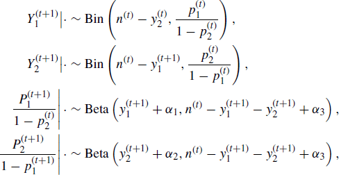
and

In Section 7.2.4 an alternative Gibbs approach uses (7.10) directly.

Example 7.5 (Bayesian Inference, Continued) The Gibbs sampler is particularly useful for Bayesian applications when the goal is to make inference based on the posterior distribution of multiple parameters. Recall Example 7.1 where the parameter vector θ has prior distribution p(θ) and likelihood function L(θ|y) arising from observed data y. Bayesian inference is based on the posterior distribution p(θ|y) = c p(θ)L(θ|y), where c is an unknown constant. When the requisite univariate conditional densities are easily sampled, the Gibbs sampler can be applied and does not require evaluation of the constant c = ∫ p(θ)L(θ|y)dθ. In this case the ith step in a cycle of the Gibbs sampler at iteration t is given by draws from

where p is the univariate conditional posterior of θ_i given the remaining parameters and the data.

Example 7.6 (Fur Seal Pup Capture–Recapture Study) By the late 1800s fur seals in New Zealand were nearly brought to extinction by Polynesian and European hunters. In recent years the abundance of fur seals in New Zealand has been increasing. This increase has been of great interest to scientists, and these animals have been studied extensively [61, 62, 405].

Our goal is to estimate the number of pups in a fur seal colony using a capture–recapture approach [585]. In such studies, separate repeated efforts are made to count a population of unknown size. In our case, the population to be counted is the population of pups. No single census attempt is likely to provide a complete enumeration of the population, nor is it even necessary to try to capture most of the individuals. The individuals captured during each census are released with a marker indicating their capture. A capture of a marked individual during any subsequent census is termed a recapture. Population size can be estimated on the basis of the history of capture and recapture data. High recapture rates suggest that the true population size does not greatly exceed the total number of unique individuals ever captured.

Let N be the unknown population size to be estimated using I census attempts yielding total numbers of captures (including recaptures) equaling . We assume that the population is closed during the period of the sampling, which means that deaths, births, and migrations are inconsequential during this period. The total number of distinct animals captured during the study is denoted by r.

We consider a model with separate, unknown capture probabilities for each census effort, . This model assumes that all animals are equally catchable on any one capture occasion, but capture probabilities may change over time. The likelihood for this model is

(7.11)

This model is sometimes called the M(t) model [55].

In a capture–recapture study conducted on the Otago Peninsula on the South Island of New Zealand, fur seal pups were marked and released during I = 7 census attempts during one season. It is reasonable to assume the population of pups was closed during the study period. Table 7.1 shows the number of pups captured (c_i) and the number of these captures corresponding to pups never previously caught (m_i), for census attempts i = 1, . . ., 7. A total of unique fur seals were observed during the sampling period.

Table 7.1 Fur seal data for seven census efforts in one season.

For estimation, one might adopt a Bayesian framework where N and α are assumed to be a priori independent with the following priors. For the unknown population size we use an improper uniform prior f(N) ∝ 1. For the capture probabilities, we use

(7.12)

for i = 1, . . ., 7, and we assume these are a priori independent. If , this corresponds to the Jeffreys prior. The combination of a uniform prior for N and a Jeffreys prior for α_i is recommended when I > 5 [653]. This leads to a proper posterior distribution for the parameters when I > 2 and there is at least one recapture (c_i − m_i > 1). A Gibbs sampler can then be constructed by simulating from the conditional posterior distributions

(7.13)

(7.14)

for i = 1, . . ., 7. Here |· denotes conditioning on the parameters among {N, α, θ₁, θ₂} as well as the data in Table 7.1, and NegBin denotes the negative binomial distribution.

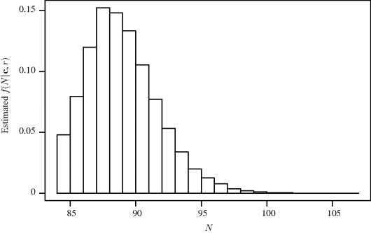
The results below are based on a chain of 100,000 iterations with the first 50,000 iterations discarded for burn-in. Diagnostics (see Example 7.10) do not indicate any problems with convergence. To investigate whether the model produces sensible results, one can compute the mean capture probability for each iteration and compare it to the corresponding simulated population size. Figure 7.6 shows split boxplots of from (7.13) for each population size N^(t) from (7.14). As expected, the population size increases as the mean probability of capture decreases. Figure 7.7 shows a histogram of the realizations of N^(t) upon which posterior inference about N is based. The posterior mean of N is 89.5 with a 95% highest posterior density (HPD) interval of (84, 94). (A 95% HPD interval for N is the region of shortest length containing 95% of the posterior probability for N for which the posterior density for every point contained in the interval is never lower than the density for every point outside the interval. See Section 7.3.3 for computational details for HPDs using MCMC.) For comparison, the maximum likelihood estimate for N is 88.5 and a 95% nonparametric bootstrap confidence interval is (85.5, 97.3).

Figure 7.6 Split boxplots of against N^(t) for the seal pup example.

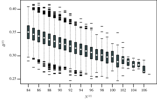
Figure 7.7 Estimated marginal posterior probabilities for N for the seal pup example.

The likelihood given in (7.11) is just one of the many forms of capture–recapture models that could have been considered. For example, a model with a common capture probability may be more appropriate. Other parameterizations of the problem might also be investigated to improve MCMC convergence and mixing, which is strongly dependent on the parameterization and updating of (θ₁, θ₂). We consider these further in Examples 7.7 and 7.10.

7.2.2 Properties of the Gibbs Sampler

Clearly the chain produced by a Gibbs sampler is Markov. Under rather mild conditions, Geman and Geman [226] showed that the stationary distribution of the Gibbs sampler chain is f. It also follows that the limiting marginal distribution of equals the univariate marginalization of the target distribution along the ith coordinate. As with the Metropolis–Hastings algorithm, we can use realizations from the chain to estimate the expectation of any function of X.

It is possible to relate the Gibbs sampler to the Metropolis–Hastings algorithm, allowing for a proposal distribution in the Metropolis–Hastings algorithm that varies over time. Each Gibbs cycle consists of p Metropolis–Hastings steps. To see this, note that the ith Gibbs step in a cycle effectively proposes the candidate vector given the current state of the chain . Thus, the ith univariate Gibbs update can be viewed as a Metropolis–Hastings step drawing

where

(7.15)

It is easy to show that in this case the Metropolis–Hastings ratio equals 1, which means that the candidate is always accepted.

The Gibbs sampler should not be applied when the dimensionality of X changes (e.g., when moving between models with different numbers of parameters at each iteration of the Gibbs sampler). Section 8.2 gives methods for constructing a suitable Markov chain with the correct stationary distribution in this case.

The “Gibbs sampler” is actually a generic name for a rich family of very adaptable algorithms. In the following subsections we describe various strategies that have been developed to improve the performance of the general algorithm described above.

7.2.3 Update Ordering

The ordering of updates made to the components of X in the basic Gibbs sampler (7.9) can change from one cycle to the next. This is called random scan Gibbs sampling [417]. Randomly ordering each cycle can be effective when parameters are highly correlated. For example, Roberts and Sahu [546] give asymptotic results for a multilevel mixed model for which a random scan Gibbs sampling approach can yield faster convergence rates than the deterministic update ordering given in (7.9). In practice without specialized knowledge for a particular model, we recommend trying both deterministic and random scan Gibbs sampling when parameters are highly correlated from one iterations to the next.

7.2.4 Blocking

Another modification to the Gibbs sampler is called blocking or grouping. In the Gibbs algorithm it is not necessary to treat each element of X individually. In the basic Gibbs sampler (7.9) with p = 4, for example, it would be allowable for each cycle to proceed with the following sequence of updates:

In Example 7.4, we saw that the stream ecology parameters were naturally grouped into a conditionally multinomial set of parameters, a conditionally Dirichlet set of parameters, and a single conditionally Poisson element (7.10). It would be convenient and correct to cycle through these blocks, sequentially sampling from multivariate instead of univariate conditional distributions in the multinomial and Dirichlet cases.

Blocking is typically useful when elements of X are correlated, with the algorithm constructed so that more correlated elements are sampled together in one block. Roberts and Sahu compare convergence rates for various blocking and update ordering strategies [546]. The structured Markov chain Monte Carlo method of Sargent et al. offers a systematic approach to blocking that is directly motivated by the model structure [569]. This method has been shown to offer faster convergence for problems with a large number of parameters, such as Bayesian analyses for longitudinal and geostatistical data [110, 124].

7.2.5 Hybrid Gibbs Sampling

For many problems the conditional distributions for one or more elements of X are not available in closed form. In this case, a hybrid MCMC algorithm can be developed where at a given step in the Gibbs sampler, the Metropolis–Hastings algorithm is used to sample from the appropriate conditional distribution. For example, for p = 5, a hybrid MCMC algorithm might proceed with the following sequence of updates:

1. Update with a Gibbs step because this conditional distribution is available in closed form.

2. Update with a Metropolis–Hasting step because this joint conditional distribution is difficult to sample from or is not available in closed form. Here, blocking X₂ and X₃ might be recommended because these elements are highly correlated.

3. Update with a step from a random walk chain because this conditional distribution is not available in closed form.

4. Update with a Gibbs step.

For both theoretical and practical reasons, only one Metropolis–Hastings step is performed at each step in the hybrid Gibbs sampler. Indeed, it has been proven that the basic Gibbs sampler in Section 7.2.1 is equivalent to the composition of p Metropolis–Hastings algorithms with acceptance probabilities equal to 1 [543]. The term “hybrid Gibbs” is rather generic terminology that is used to describe many different algorithms (see Section 8.4 for more examples). The example shown in steps 1–4 above is more precisely described as a“hybrid Gibbs sampler with Metropolis steps within Gibbs,” which is sometimes abbreviated as “Metropolis-within-Gibbs,” and was first proposed by [472].

Example 7.7 (Fur Seal Pup Capture–Recapture Study, Continued) Example 7.6 described the M(t) model in (7.11) for capture–recapture studies. For this model a common practice is to assume a Beta prior distribution for the capture probabilities and a noninformative Jeffreys prior for N, so f(N) ∝ 1/N. For some datasets, previous analyses have shown sensitivity to the values selected for θ₁ and θ₂ in (7.12) [230]. To mitigate this sensitivity, we consider an alternative setup with a joint distribution for (θ₁, θ₂), namely with (θ₁, θ₂) assumed to be a priori independent of the remaining parameters. A Gibbs sampler can then be constructed by simulating from the conditional posterior distributions

(7.16)

(7.17)

(7.18)

where |· denotes conditioning on the remaining parameters from {N, α, θ₁, θ₂} as well as the data in Table 7.1 and k is an unknown constant. Note that (7.18) is not easy to sample. This suggests using a hybrid Gibbs sampler with a Metropolis–Hastings step for (7.18). Thus the Gibbs sampler in (7.13)–(7.14) becomes a hybrid Gibbs sampler in (7.16)–(7.18) when a prior distribution is used for θ₁ and θ₂ instead of selecting values for these parameters.

7.2.6 Griddy–Gibbs Sampler

Hybrid methods such as embedding Metropolis–Hastings steps within a Gibbs algorithm are one way to construct a Gibbs-like chain when not all the univariate conditionals are easily sampled. Other strategies, evolved from techniques in Chapter 6, can be used to sample difficult univariate conditionals.

One such method is the griddy–Gibbs sampler [541, 624]. Suppose that it is difficult to sample from the univariate conditional density for X_k|x_−k for a particular k. To implement a griddy–Gibbs step, select some grid points z₁, . . ., z_n over the range of support of f(· |x_−k). Let for j = 1, . . ., n. Using these weights and the corresponding grid, one can approximate the density function f(· |x_−k) or, equivalently, its inverse cumulative distribution function. Generate from this approximation, and proceed with the remainder of the MCMC algorithm. The approximation to the kth univariate conditional can be refined as iterations proceed. The simplest approach for the approximation and sampling step is to draw from the discrete distribution on z₁, . . ., z_n with probabilities proportional to , using the inverse cumulative distribution function method (Section 6.2.2). A piecewise linear cumulative distribution function could be generated from an approximating density function that is piecewise constant between the midpoints of any two adjacent grid values with a density height set to ensure that the total probability on the segment containing z_i is proportional to . Other approaches could be based on the density estimation ideas presented in Chapter 10.

If the approximation to f(· |x_−k) is updated from time to time by improving the grid, then the chain is not time homogeneous. In this case, reference to convergence results for Metropolis–Hastings or Gibbs chains is not sufficient to guarantee that a griddy–Gibbs chain has a limiting stationary distribution equal to f. One way to ensure time homogeneity is to resist making any improvements to the approximating univariate distribution as iterations progress. In this case, however, the limiting distribution of the chain is still not correct because it relies on an approximation to f(· |x_−k) rather than the true density. This can be corrected by reverting to a hybrid Metropolis-within-Gibbs framework where the variable generated from the approximation to f(· |x_−k) is viewed as a proposal, which is then randomly kept or discarded based on the Metropolis–Hastings ratio. Tanner discusses a wide variety of potential enhancements to the basic griddy–Gibbs strategy [624].

7.3 Implementation

The goal of an MCMC analysis is to estimate features of the target distribution f. The reliability of such estimates depends on the extent to which sample averages computed using realizations of the chain correspond to their expectation under the limiting stationary distribution of the chain. Aside from griddy–Gibbs, all of the MCMC methods described above have the correct limiting stationary distribution. In practice, however, it is necessary to determine when the chain has run sufficiently long so that it is reasonable to believe that the output adequately represents the target distribution and can be used reliably for estimation. Unfortunately, MCMC methods can sometimes be quite slow to converge, requiring extremely long runs, especially if the dimensionality of X is large. Further, it is often easy to be misled when using MCMC algorithm output to judge whether convergence has approximately been obtained.

In this section, we examine questions about the long-run behavior of the chain. Has the chain run long enough? Is the first portion of the chain highly influenced by the starting value? Should the chain be run from several different starting values? Has the chain traversed all portions of the region of support of f? Are the sampled values approximate draws from f? How shall the chain output be used to produce estimates and assess their precision? Useful reviews of MCMC diagnostic methods include [76, 125, 364, 458, 543, 544]. We end with some practical advice for coding MCMC algorithms.

7.3.1 Ensuring Good Mixing and Convergence

It is important to consider how efficiently an MCMC algorithm provides useful information about a problem of interest. Efficiency can take on several meanings in this context, but here we will focus on how quickly the chain forgets its starting value and how quickly the chain fully explores the support of the target distribution. A related concern is how far apart in a sequence observations need to be before they can be considered to be approximately independent. These qualities can be described as the mixing properties of the chain.

We must also be concerned whether the chain has approximately reached its stationary distribution. There is substantial overlap between the goals of diagnosing convergence to the stationary distribution and investigating the mixing properties of the chain. Many of the same diagnostics can be used to investigate both mixing and convergence. In addition, no diagnostic is fail-safe; some methods can suggest that a chain has approximately converged when it has not. For these reasons, we combine the discussion of mixing and convergence in the following subsections, and we recommend that a variety of diagnostic techniques be used.

7.3.1.1 Simple Graphical Diagnostics

After programming and running the MCMC algorithm from multiple starting points, users should perform various diagnostics to investigate the properties of the MCMC algorithm for the particular problem. Three simple diagnostics are discussed below.

A sample path is a plot of the iteration number t versus the realizations of X^(t). Sample paths are sometimes called trace or history plots. If a chain is mixing poorly, it will remain at or near the same value for many iterations, as in the lower panel in Figure 7.2. A chain that is mixing well will quickly move away from its starting value and the sample path will wiggle about vigorously in the region supported by f.

The cumulative sum (cusum) diagnostic assesses the convergence of an estimator of a one-dimensional parameter θ = E{h(X)} [678]. For n realizations of the chain after discarding some initial iterates, the estimator is given by . The cusum diagnostic is a plot of versus t. If the final estimator will be computed using only the iterations of the chain that remain after removing some burn-in values (see Section 7.3.1.2), then the estimator and cusum plot should be based only on the values to be used in the final estimator. Yu and Mykland [678] suggest that cusum plots that are very wiggly and have smaller excursions from 0 indicate that the chain is mixing well. Plots that have large excursions from 0 and are smoother suggest slower mixing speeds. The cusum plot shares one drawback with many other convergence diagnostics: For a multimodal distribution where the chain is stuck in one of the modes, the cusum plot may appear to indicate good performance when, in fact, the chain is not performing well.

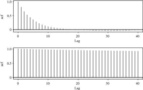
An autocorrelation plot summarizes the correlation in the sequence of X^(t) at different iteration lags. The autocorrelation at lag i is the correlation between iterates that are i iterations apart [212]. A chain that has poor mixing properties will exhibit slow decay of the autocorrelation as the lag between iterations increases. For problems with more than one parameter it may also be of use to consider cross-correlations between parameters that might be related, since high cross-correlations may also indicate poor mixing of the chain.

Example 7.8 (Mixture Distribution, Continued) Figure 7.8 shows autocorrelation function (acf) plots for the independence chain described in Example 7.2. In the top panel, the more appropriate proposal distribution yields a chain for which the autocorrelations decrease rather quickly. In the lower panel, the bad proposal distribution yields a chain for which autocorrelations are very high, with a correlation of 0.92 for observations that are 40 iterations apart. This panel clearly indicates poor mixing.

Figure 7.8 Autocorrelation function plots for independence chain of Example 7.2 with proposal densities Beta(1,1) (top) and Beta(2,10) (bottom).

7.3.1.2 Burn-in and Run Length

Key considerations in the diagnosis of convergence are the burn-in period and run length. Recall that it is only in the limit that an MCMC algorithm yields X^(t) ~ f. For any implementation, the iterates will not have exactly the correct marginal distribution, and the dependence on the initial point (or distribution) from which the chain was started may remain strong. To reduce the severity of this problem, the first D values from the chain are typically discarded as a burn-in period.

A commonly used approach for the determination of an appropriate burn-in period and run length is that of Gelman and Rubin [221, 224]. This method is based on a statistic motivated by an analysis of variance (ANOVA): The burn-in period or MCMC run-length should be increased if a between-chain variance is considerably larger than the within-chain variance. The variances are estimated based on the results of J runs of the MCMC algorithm to create separate, equal-length chains (J ≥ 2) with starting values dispersed over the support of the target density.

Let L denote the length of each chain after discarding D burn-in iterates. Suppose that the variable (e.g., parameter) of interest is X, and its value at the tth iteration of the jth chain is . Thus, for the jth chain, the D values are discarded and the L values are retained. Let

(7.19)

and define the between-chain variance as

(7.20)

Next define

to be the within-chain variance for the jth chain. Then let

(7.21)

represent the mean of the J within-chain estimated variances. Finally, let

(7.22)

If all the chains are stationary, then both the numerator and the denominator should estimate the marginal variance of X. If, however, there are notable differences between the chains, then the numerator will exceed the denominator.

In theory, as L→ ∞. In practice, the numerator in (7.22) is slightly too large and the denominator is slightly too small. An adjusted estimator is given by

Some authors suggest that indicates that the burn-in and chain length are sufficient [544]. Another useful convergence diagnostic is a plot of the values of versus the number of iterations. When has not stabilized near 1, this suggests lack of convergence. If the chosen burn-in period did not yield an acceptable result, then D should be increased, L should be increased, or preferably both. A conservative choice is to use one-half of the iterations for burn-in. The performance of this diagnostic is improved if the iterates are transformed so that their distribution is approximately normal. Alternatively, a reparameterization of the model could be undertaken and the chain rerun.

There are several potential difficulties with this approach. Selecting suitable starting values in cases of multimodal f may be difficult, and the procedure will not work if all of the chains become stuck in the same subregion or mode. Due to its unidimensionality, the method may also give a misleading impression of convergence for multidimensional target distributions. Enhancements of the Gelman–Rubin statistic are described in [71, 224], including an improved estimate of R in (7.22) that accounts for variability in unknown parameters. In practice, these improvements lead to very similar results. An extension for multidimensional target distributions is given in [71].

Raftery and Lewis [526] proposed a very different quantitative strategy for estimating run length and burn-in period. Some researchers advocate no burn-in [231].

7.3.1.3 Choice of Proposal

As illustrated in Example 7.2, mixing is strongly affected by features of the proposal distribution, especially its spread. Further, advice on desirable features of a proposal distribution depends on the type of MCMC algorithm employed.

For a general Metropolis–Hastings chain such as an independence chain, it seems intuitively clear that we wish the proposal distribution g to approximate the target distribution f very well, which in turn suggests that a very high rate of accepting proposals is desirable. Although we would like g to resemble f, the tail behavior of g is more important than its resemblance to f in regions of high density. In particular, if f/g is bounded, the convergence of the Markov chain to its stationary distribution is faster overall [543]. Thus, it is wiser to aim for a proposal distribution that is somewhat more diffuse than f.

In practice, the variance of the proposal distribution can be selected through an informal iterative process. Start a chain, and monitor the proportion of proposals that have been accepted; then adjust the spread of the proposal distribution accordingly. After some predetermined acceptance rate is achieved, restart the chain using the appropriately scaled proposal distribution. For a Metropolis algorithm with normal target and proposal distributions, it has been suggested that an acceptance rate of between 25 and 50% should be preferred, with the best choice being about 44% for one-dimensional problems and decreasing to about 23.4% for higher-dimensional problems [545, 549]. To apply such rules, care are must be taken to ensure that the target and proposal distributions are roughly normally distributed or at least simple, unimodal distributions. If, for example, the target distribution is multimodal, the chain may get stuck in one mode without adequate exploration of the other portions of the parameter space. In this case the acceptance rate may very high, but the probability of jumping from one mode to another may be low. This suggests one difficult issue with most MCMC methods; it is useful to have as much knowledge as possible about the target distribution, even though that distribution is typically unknown.

Methods for adaptive Markov chain Monte Carlo (Section 8.1) tune the proposal distribution in the Metropolis algorithm during the MCMC algorithm. These methods have the advantage that they are automatic and, in some implementations, do not require the user to stop, tune, and restart the algorithm on multiple occasions.

7.3.1.4 Reparameterization

Model reparameterization can provide substantial improvements in the mixing behavior of MCMC algorithms. For a Gibbs sampler, performance is enhanced when components of X are as independent as possible. Reparameterization is the primary strategy for reducing dependence. For example, if f is a bivariate normal distribution with very strong positive correlation, both univariate conditionals will allow only small steps away from X^(t) = x^(t) along one axis. Therefore, the Gibbs sampler will explore f very slowly. However, suppose . This transformation yields one univariate conditional on the axis of maximal variation in X and the second on an orthogonal axis. If we view the support of f as cigar shaped, then the univariate conditionals for Y allow one step along the length of the cigar, followed by one across its width. Therefore, the parameterization inherent in Y makes it far easier to move from one point supported by the target distribution to any other point in a single move (or a few moves).

Different models require different reparameterization strategies. For example, if there are continuous covariates in a linear model, it is useful to center and scale the covariates to reduce correlations between the parameters in the model. For Bayesian treatment of linear models with random effects, hierarchical centering can be used to accelerate MCMC convergence [218, 219]. The term hierarchical centering comes from the idea that the parameters are centered as opposed to centering the covariates. Hierarchical centering involves reexpressing a linear model into another form that produces different conditional distributions for the Gibbs sampler.

Example 7.9 (Hierarchical Centered Random Effects Model) For example, consider a study of pollutant levels where it is known that tests performed at different laboratories have different levels of measurement error. Let y_ij be the pollutant level of the jth sample that was tested at the ith laboratory. We might consider a simple random effects model

(7.23)

where i = 1, . . ., I and j = 1, . . ., n_i. In the Bayesian paradigm, we might assume , , and . The hierarchical centered form of (7.23) is a simple reparameterization of the model with y_ij = γ_i + _ij where γ_i = μ + α_i and . Thus γ is centered about μ. Hierarchical centering usually produces better behaved MCMC chains when is not a lot larger than , which is likely when random effects are deemed useful for modeling a given dataset. While this is a simple example, hierarchical centering has been shown to produce more efficient MCMC algorithms for more complex linear model problems such as generalized linear mixed models. However, the advantages of hierarchical centering can depend on the problem at hand and should be implemented on a case-by-case basis [77, 219]. See Problems 7.7 and 7.8 for another example of hierarchical centering.

Unfortunately, reparameterization approaches are typically adapted for specific models, so it is difficult to provide generic advice. Another way to improve mixing and accelerate convergence of MCMC algorithms is to augment the problem using so-called auxiliary variables; see Chapter 8. A variety of reparameterization and acceleration techniques are described in [106, 225, 242, 543].

7.3.1.5 Comparing Chains: Effective Sample Size

If MCMC realizations are highly correlated, then the information gained from each iteration of the MCMC algorithm will be much less than suggested by the run length. The reduced information is equivalent to that contained in a smaller i.i.d. sample whose size is called the effective sample size. The difference between the total number of samples and the effective sample size indicates the efficiency lost when correlated samples from the Markov chain have been used to estimate a quantity of interest instead of an independent and identically distributed sample with the same variance as the observed sample [543].

To estimate the effective sample size, the first step is to compute the estimated autocorrelation time, a summary measure of the autocorrelation between realizations and their rate of decay. The autocorrelation time is given by

(7.24)

where ρ(k) is the autocorrelation between realizations that are k iterations apart (e.g., the correlation between X^(t) and X^(t+k) for t = 1, . . ., L). Accurate estimation of ρ(k) presents its own challenges, but a common approach is to truncate the summation when [110]. Then the effective sample size for an MCMC run with L iterations after burn-in can be estimated using .

Effective sample size can be used to compare the efficiency of competing MCMC samplers for a given problem. For a fixed number of iterations, an MCMC algorithm with a larger effective sample size is likely to converge more quickly. For example, we may be interested in the gains achieved from blocking in a Gibbs sampler. If the blocked Gibbs sampler has a much higher effective sample size than the unblocked version, this suggests that the blocking has improved the efficiency of the MCMC algorithm. Effective sample size can also be used for a single chain. For example, consider a Bayesian model with two parameters (α, β) and an MCMC algorithm run for 10,000 iterations after burn-in. An effective sample size of, say, 9500 iterations for α suggests low correlations between iterations. In contrast, if the results indicated an effective sample size of 500 iterations for β, this would suggest that convergence for β is highly suspect.

7.3.1.6 Number of Chains

One of the most difficult problems to diagnose is whether or not the chain has become stuck in one or more modes of the target distribution. In this case, all convergence diagnostics may indicate that the chain has converged, though the chain does not fully represent the target distribution. A partial solution to this problem is to run multiple chains from diverse starting values and then compare the within-and between-chain behavior. A formal approach for doing this is described in Section 7.3.1.2.

The general notion of running multiple chains to study between-chain performance is surprisingly contentious. One of the most vigorous debates during the early statistical development of MCMC methods centered around whether it was more important to invest limited computing time in lengthening the run of a single chain, or in running several shorter chains from diverse starting points to check performance [224, 233, 458]. The motivation for trying multiple runs is the hope that all interesting features (e.g., modes) of the target distribution will be explored by at least one chain, and that the failure of individual chains to find such features or to wash out the influence of their starting values can be detected, in which case chains must be lengthened or the problem reparameterized to encourage better mixing.

Arguments for one long chain include the following. Many short runs are more informative than one long run only when they indicate poor convergence behavior. In this case, the simulated values from the many short chains remain unusable. Second, the effectiveness of using many short runs to diagnose poor convergence is mainly limited to unrealistically simple problems or problems where the features of f are already well understood. Third, splitting computing effort into many short runs may yield an indication of poor convergence that would not have occurred if the total computing effort had been devoted to one longer run.

We do not find the single-chain arguments entirely convincing from a practical point of view. Starting a number of shorter chains from diverse starting points is an essential component of thorough debugging of computer code. Some primary features of f (e.g., multimodality, highly constrained support region) are often broadly known—even in complex realistic problems—notwithstanding uncertainty about specific details of these features. Results from diverse starts can also provide information about key features of f, which in turn helps determine whether the MCMC method and problem parameterization are suitable. Poor convergence of several short chains can help determine what aspects of chain performance will be most important to monitor when a longer run is made. Finally, CPU cycles are more abundant and less expensive than they were a decade ago. We can have diverse short runs and one longer run. Exploratory work can be carried out using several shorter chains started from various points covering the believed support of f. Diagnosis of chain behavior can be made using a variety of informal and formal techniques, using the techniques described in this chapter. After building confidence that the implementation is a promising one, it is advisable to run one final very long run from a good starting point to calculate and publish results.

7.3.2 Practical Implementation Advice

The discussion above raises the question of what values should be used for the number of chains, the number of iterations for burn-in, and the length of the chain after burn-in. Most authors are reluctant to recommend generic values because appropriate choices are highly dependent on the problem at hand and the rate and efficiency with which the chain explores the region supported by f. Similarly, the choices are limited by how much computing time is available. Published analyses have used burn-ins from zero to tens of thousands and chain lengths from the thousands to the millions. Diagnostics usually rely on at least three, and typically more, multiple chains. As computing power continues to grow, so too will the scope and intensity of MCMC efforts.

In summary, we reiterate our advice from Section 7.3.1.6 here, which in turn echoes [126]. First, create multiple trial runs of the chain from diverse starting values. Next, carry out a suite of diagnostic procedures like those discussed above to ensure that the chain appears to be well mixing and has approximately converged to the stationary distribution. Then, restart the chain for a final long run using a new seed to initiate the sampling. A popular, though conservative, choice for burn-in is to throw out the first half of the MCMC iterations as the burn-in. When each MCMC iteration is computationally expensive, users typically select much shorter burn-in lengths that conserve more iterations for inference.

For learning about MCMC methods and chain behavior, nothing beats programming these algorithms from scratch. For easier implementation, various software packages have been developed to automate the development of MCMC algorithms and the related diagnostics. The most comprehensive software to date is the BUGS (Bayesian inference Using Gibbs Sampling) software family with developments for several platforms [610]. A popular application mode is to use BUGS within the R statistical package [626]. Packages in R like CODA [511] and BOA [607] allow users to easily construct the relevant convergence diagnostics. Most of this software is freely available via the Internet.

7.3.3 Using the Results

We describe here some of the common summaries of MCMC algorithm output and continue the fur seal pup example for further illustration.

The first topic to consider is marginalization. If {X^(t)} represents a p-dimensional Markov chain, then is a Markov chain whose limiting distribution is the ith marginal of f. If you are focused only on a property of this marginal, discard the rest of the simulation and analyze the realizations of . Further, note that it is not necessary to run a chain for every quantity of interest. Post hoc inference about any quantity can be obtained from the realizations of X^(t) generated by the chain. In particular, the probability for any event can be estimated by the frequency of that event in the chain.

Standard one-number summary statistics such as means and variances are commonly desired (see Section 7.1). The most commonly used estimator is based on an empirical average. Discard the burn-in; then calculate the desired statistic by taking

(7.25)

as the estimator of E{h(X)}, where L denotes the length of each chain after discarding D burn-in iterates. This estimator is consistent even though the X^(t) are serially correlated. There are asymptotic arguments in favor of using no burn-in (so D = 1) [231]. However, since a finite number of iterations is used to compute the estimator in (7.25), most researchers employ a burn-in to reduce the influence of the initial iterates sampled from a distribution that may be far from the target distribution. We recommend using a burn-in period.

Other estimators have been developed. The Riemann sum estimator in (6.86) has been shown to have faster convergence than the standard estimator given above. Other variance reduction techniques discussed in Section 6.4, such as Rao–Blackwellization, can also be used to reduce the Monte Carlo variability of estimators based on the chain output [507].

The Monte Carlo, or simulation, standard error of an estimator is also of interest. This is an estimate of the variability in the estimator if the MCMC algorithm were to be run repeatedly. The naive estimate of the standard error for an estimator like (c07-mdis-0033) is the sample standard deviation of the L realizations after burn-in divided by . However, MCMC realizations are typically positively correlated, so this can underestimate the standard error. An obvious correction is to compute the standard error based on a systematic subsample of, say, every kth iterate after burn-in. However, this approach is inefficient [429]. A simple estimator of the standard error is the batch method [92, 324]. Separate the L iterates into batches with b consecutive iterations in each batch. Compute the mean of each batch. Then the estimated standard error is the standard deviation of these means divided by the square root of the number of batches. A recommended batch size is b = L^1/a where a = 2 or 3 and z denotes the largest integer less than z [355]. Other strategies to estimate Monte Carlo standard errors are surveyed in [196, 233, 609]. The Monte Carlo standard error can be used to assess the between-simulation variability. It has been suggested that, after determining that the chain has good mixing and convergence behavior, you should run the chain until the Monte Carlo simulation error is less than 5% of the standard deviation for all parameters of interest [610].

Quantile estimates and other interval estimates are also commonly desired. Estimates of various quantiles such as the median or the fifth percentile of h(X) can be computed using the corresponding percentile of the realizations of the chain. This is simply implementing (7.25) for tail probabilities and inverting the relationship to find the quantile.

For Bayesian analyses, computation of the highest posterior density (HPD) interval is often of interest (see Section 1.5). For a unimodal and symmetric posterior distribution, the (1 − α)% HPD interval is given by the (α/2)th and (1 − α/2)th percentiles of the iterates. For a unimodal posterior distribution, an MCMC approximation of the HPD interval can be computed as follows. For the parameter of interest, sort the MCMC realizations after burn-in, x^(D), . . ., x^(D+L−1) to obtain x₍₁₎ ≤ x₍₂₎ . . . ≤ x_(L−1). Compute the 100(1 − α)% credible intervals

where z represents the largest integer not greater than z. The 100(1 − α)% HPD interval is the interval with the shortest interval width among all credible intervals [107]. More sophisticated alternatives for HPD computation for multimodal posterior densities and other complexities are given in [106].

Simple graphical summaries of MCMC output should not be overlooked. Histograms of the realizations of h(X^(t)) for any h of interest are standard practice. Alternatively, one can apply one of the density estimation techniques from Chapter 10 to summarize the collection of values. It is also common practice to investigate pairwise scatterplots and other descriptive plots to explore or illustrate key features of f.

Example 7.10 (Fur Seal Pup Capture–Recapture Study, Continued) Recall the fur seal pup capture–recapture study in Example 7.6 that led to the Gibbs sampler summarized in (7.13) and (7.14). A hybrid Gibbs sampler for this problem is considered in Example 7.7. When applied to the fur seal data these MCMC algorithms have very different performance. We will consider these two variations to demonstrate the MCMC diagnostics described above.

For the basic Gibbs sampler in Example 7.6, the sample path and autocorrelation plots do not indicate any lack of convergence (Figure 7.9). Based on five runs of 100,000 iterations each with a burn-in of 50,000, the Gelman–Rubin statistic for N is equal to 0.999995, which suggests the N^(t) chain is roughly stationary. The effective sample size was 45,206 samples (iterations). Similarly, for the hybrid sampler in Example 7.7 there is no evidence of lack of convergence for N, so we will not consider this parameter further.

Figure 7.9 Output from the basic Gibbs sampler from Example 7.6. Top row: sample paths for last 1000 iterations of N (left) and α₁ (right). Bottom row: autocorrelation plots after burn-in for N (left) and α₁ (right).

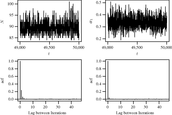
In contrast to the speedy convergence for N, MCMC convergence behavior for the capture probability parameters (α₁, . . ., α₇) varies with the form of the model and Gibbs sampling strategy. For the uniform/Jeffreys prior combination and basic Gibbs sampler in Example 7.6, the Gelman–Rubin statistic for the capture probabilities are all close to one, and the capture probabilities exhibit little correlation between MCMC samples (e.g., lower right panel of Figure 7.9). This suggests that the chains are roughly stationary. However, as we will show below, the alternative prior distributions and the hybrid Gibbs sampler described in Example 7.7 lead to less satisfactory MCMC convergence behavior.

To implement the hybrid Gibbs sampler for Example 7.7, a Metropolis–Hastings step is required to sample (θ₁, θ₂) in (7.18). Note that the prior distribution for these parameters restricts (θ₁, θ₂) to be larger than 0. Such a constraint can impede MCMC performance, particularly if there is high posterior density near the boundary. Therefore we consider using a random walk to update these parameters, but to improve performance we transform (θ₁, θ₂) to U = (U₁, U₂) = (log θ₁, log θ₂). This permits a random walk step on (− ∞, ∞) to update U effectively. Specifically, proposal values U^∗ can be generated by drawing ~ N(0, 0 . 085²I) where I is the 2 × 2 identity matrix and then setting U^∗ = u^(t) + . We select a standard deviation of 0.085 to get an acceptance rate of about 23% for the U updates. Recalling (7.8) in Example 7.3, it is necessary to transform (7.17) and (7.18) to reflect the change of variables. Thus, (7.17) becomes

(7.26)

and (7.18) becomes

(7.27)

where k_u is an unknown constant. This method of transforming the parameter space via a change-of-variables method within the Metropolis–Hastings algorithm is useful for problems with constrained parameter spaces. The idea is to transform the constrained parameters so that the MCMC updates can be made on . See [329] for a more complex example.

We implement the hybrid sampler running a chain of 100,000 iterations with the first 50,000 iterations discarded for burn-in. The Gelman–Rubin statistics for the parameters are all very close to 1, however, the autocorrelation plots indicate high correlation between iterations (left panel in Figure 7.10). For example, using the alternative prior distributions and the hybrid Gibbs sampler produces correlations of 0.6 between MCMC samples that are 40 iterations apart as compared to correlations near 0 at lags of 2 when using the uniform/Jeffreys prior combination and basic Gibbs sampler shown in Figure 7.9. Similarly, the effective sample size for the hybrid Gibbs algorithm of 1127 can be compared to the much larger effective sample size of 45,206 in the basic Gibbs sampler discussed above. The right panel of Figure 7.10 shows the bivariate sample path of and for the hybrid sampler. This plot indicates a high correlation between the parameters. These results suggest a lack of convergence of the MCMC algorithm or at least poor behavior of the chain for the hybrid algorithm. In spite of these indications of lack of convergence, the prior distributions from Example 7.7 produce very similar results to those from the uniform/Jeffreys prior combination for Example 7.6. The posterior mean of N is 90 with a 95% HPD interval of (85, 95). However, the chain does not mix as well as the simpler model, so we prefer the uniform/Jeffreys prior for the seal pup data. A hybrid Gibbs sampler can be quite effective for many problems, but for these data the alternative prior described in Example 7.7 is not appropriate and the hybrid algorithm does not remedy the problem.

Figure 7.10 For the hybrid Gibbs sampler from Example 7.7: Autocorrelation function plot for p₁ (left panel) and sample path for U (right panel) for final 5000 iterations in the seal pup example.

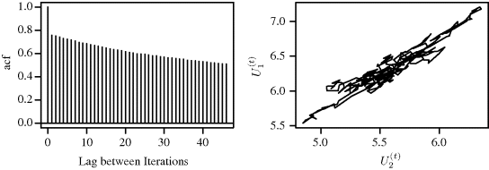
Problems

7.1. The goal of this problem is to investigate the role of the proposal distribution in a Metropolis–Hastings algorithm designed to simulate from the posterior distribution of a parameter δ. In part (a), you are asked to simulate data from a distribution with δ known. For parts (b)–(d), assume δ is unknown with a Unif(0,1) prior distribution for δ. For parts (b)–(d), provide an appropriate plot and a table summarizing the output of the algorithm. To facilitate comparisons, use the same number of iterations, random seed, starting values, and burn-in period for all implementations of the algorithm.

a. Simulate 200 realizations from the mixture distribution in Equation (7.6) with δ = 0.7. Draw a histogram of these data.

b. Implement an independence chain MCMC procedure to simulate from the posterior distribution of δ, using your data from part (a).

c. Implement a random walk chain with δ^∗ = δ^(t) + with ~Unif(−1,1).

d. Reparameterize the problem letting U = log {δ/(1 − δ)} and U^∗ = u^(t) + . Implement a random walk chain in U-space as in Equation (7.8).

e. Compare the estimates and convergence behavior of the three algorithms.

7.2. Simulating from the mixture distribution in Equation (7.6) is straightforward [see part (a) of Problem 7.1]. However, using the Metropolis–Hastings algorithm to simulate realizations from this distribution is useful for exploring the role of the proposal distribution.

7.3. Consider a disk D of radius 1 inscribed within a square of perimeter 8 centered at the origin. Then the ratio of the area of the disk to that of the square is π/4. Let f represent the uniform distribution on the square. Then for a sample of points (X_i, Y_i) ~ f(x, y) for i = 1, . . ., n, is an estimator of π (where 1_{A} is 1 if A is true and 0 otherwise).

Consider the following strategy for estimating π. Start with (x⁽⁰⁾, y⁽⁰⁾) = (0, 0). Thereafter, generate candidates as follows. First, generate Unif(− h, h) and Unif(− h, h). If falls outside the square, regenerate and until the step taken remains within the square. Let . Increment t. This generates a sample of points over the square. When t = n, stop and calculate as given above.

a. Implement this method for h = 1 and n = 20, 000. Compute . What is the effect of increasing n? What is the effect of increasing and decreasing h? Comment.

b. Explain why this method is flawed. Using the same method to generate candidates, develop the correct approach by referring to the Metropolis–Hastings ratio. Prove that your sampling approach has a stationary distribution that is uniform on the square.

c. Implement your approach from part (b) and calculate . Experiment again with n and h. Comment.

7.4. Derive the conditional distributions in Equation (7.10) and the univariate conditional distributions below Equation (7.10).

7.5. A clinical trial was conducted to determine whether a hormone treatment benefits women who were treated previously for breast cancer. Each subject entered the clinical trial when she had a recurrence. She was then treated by irradiation and assigned to either a hormone therapy group or a control group. The observation of interest is the time until a second recurrence, which may be assumed to follow an exponential distribution with parameter τθ (hormone therapy group) or θ (control group). Many of the women did not have a second recurrence before the clinical trial was concluded, so that their recurrence times are censored.

In Table 7.2, a censoring time M means that a woman was observed for M months and did not have a recurrence during that time period, so that her recurrence time is known to exceed M months. For example, 15 women who received the hormone treatment suffered recurrences, and the total of their recurrence times is 280 months.

Table 7.2 Breast cancer data.

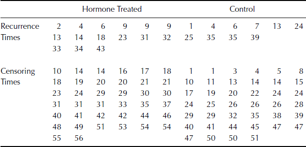
Let be the data for the ith person in the hormone group, where is the time and equals 1 if is a recurrence time and 0 if a censored time. The data for the control group can be written similarly.

The likelihood is then

You've been hired by the drug company to analyze their data. They want to know if the hormone treatment works, so the task is to find the marginal posterior distribution of τ using the Gibbs sampler. In a Bayesian analysis of these data, use the conjugate prior

Physicians who have worked extensively with this hormone treatment have indicated that reasonable values for the hyperparameters are (a, b, c, d) = (3, 1, 60, 120).

7.6. Problem 6.4 introduces data on coal-mining disasters from 1851 to 1962. For these data, assume the model

(7.28)

Assume λ_i|α ~ Gamma (3, α) for i = 1, 2, where α ~ Gamma(10, 10), and assume θ follows a discrete uniform distribution over {1, . . ., 111}. The goal of this problem is to estimate the posterior distribution of the model parameters via a Gibbs sampler.

7.7. Consider a hierarchical nested model

(7.29)

where i = 1, . . ., I, j = 1, . . ., J_i, and k = 1, . . ., K. After averaging over k for each i and j, we can rewrite the model (7.29) as

(7.30)

where . Assume that , , and , where each set of parameters is independent a priori. Assume that , , and are known. To carry out Bayesian inference for this model, assume an improper flat prior for μ, so f(μ) ∝ 1. We consider two forms of the Gibbs sampler for this problem [546]:

a. Let n = ∑ _iJ_i, y_·· = ∑ _ijy_ij/n, and y_i· = ∑ _jy_ij/J_i hereafter. Show that at iteration t, the conditional distributions necessary to carry out Gibbs sampling for this model are given by

where

b. The convergence rate for a Gibbs sampler can sometimes be improved via reparameterization. For this model, the model can be reparameterized via hierarchical centering (Section 7.3.1.4). For example, let Y_ij follow (7.30), but now let η_ij = μ + α_i + β_j(i) and . Then let γ_i = μ + α_i with and . As above, assume , , and are known, and assume a flat prior for μ. Show that the conditional distributions necessary to carry out Gibbs sampling for this model are given by

where

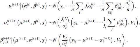
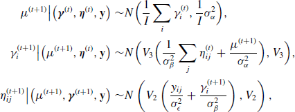
7.8. In Problem 7.7, you were asked to derive Gibbs samplers under two model parameterizations. The goal of this problem is to compare the performance of the samplers.

The website for this book provides a dataset on the moisture content in the manufacture of pigment paste [58]. Batches of the pigment were produced, and the moisture content of each batch was tested analytically. Consider data from 15 randomly selected batches of pigment. For each batch, two independent samples were randomly selected and each of these samples was measured twice. For the analyses below, let , , and .

Implement the two Gibbs samplers described below. To facilitate comparisons between the samplers, use the same number of iterations, random seed, starting values, and burn-in period for both implementations.

7.9. Example 7.10 describes the random walk implementation of the hybrid Gibbs sampler for the fur seal pup capture–recapture study. Derive the conditional distributions required for the Gibbs sampler, Equations (7.26) and (7.27).