15
Standard Costing
CHAPTER OUTLINE
LEARNING OBJECTIVES
After reading this chapter, you should be able to:
Understand standard costing: its meaning and definition
Learn the advantages and limitations of standard costing
Learn how to set standards and determinations
Learn how to revise standards
15.1 INTRODUCTION
Standard costing is a technique to control costs. It aims at increasing efficiency in performance through setting up standards. Standard costing is also known as variance analysis. It studies variances between the standard and actual.
The Institute of Cost and Management Accountants (CIMA), London, defines standard cost as ‘a predetermined cost which is calculated from management's standards of efficient operations and the relevant necessary expenditure’.
Standard cost is the predetermined cost of manufacturing a single unit or a number of product units. It is the planned cost of a product.
15.2 ADVANTAGES OF STANDARD COSTING
The advantages of standard costing are as follows:
- Efficiency measurement: The comparison of actual costs with standard costs enables managements to evaluate the performance of various departments.
- Cost control: Every costing system aims at cost control. Whenever a variance occurs, the reasons are studied and immediate corrective measures are taken.
- Right decisions: It provides useful information to the management in making important decisions.
- Eliminating inefficiencies: Standard costing aims at eliminating inefficiencies at different levels of management through various steps.
15.3 LIMITATIONS OF STANDARD COSTING
The limitations of standard costing are as follows:
- Standard costing cannot be used in organizations where non–standard products are produced.
- The process of setting standards is a difficult task as it requires technical skills.
- If standards are not revised with changes in circumstances, the same become impracticable.
- Standard costing is applicable in circumstances where variances are controllable.
15.4 MATERIAL VARIANCE
Material variance can be analysed as follows:
- Material cost variance (MCV)
- Material price variance (MPV)
- Material usage/quantity variance (MUV)
- Material mix variance (MMV)
- Material yield (sub–usage) variance (MYV)
The formulae for the aforementioned variances are as follows:
MCV = (standard quantity [SQ] × standard price [SP]) – (actual quantity [AQ] × actual price [AP])
MPV = AQ (standard rate [SR] – actual rate [AR])
MUV = SR (SQ – AQ)
MMV = SR (SQ – AQ) or (revised SQ [RSQ] – AQ)
MYV = SR (actual yield [AY] – standard yield [SY])
These variances can be defined as follows:
- MCV: MCV = standard cost of materials for actuual output – actual cost of materials used
or
MCV = MPV + MUVor
MCV = MPV + MMV + MYV - MPV: MPV = actual usage (standard unit price – actual unit price)
Here, actual usage = AQ of material (in units) used
Standard unit price = SP of material per unit
Actual unit price = AP of material per unit
- MQV: MQV = standard price per unit (standard quantity – actual quantity)
- MMV : In case of MMV, two situations may arise:
- Actual weight of mix and standard weight of mix are not different. In such a case, MMV is calculated with the help of the following formula:
MMV = standard unit cost (standard quantity – actual quantity)
or
MMV = standard cost of standard mix – standard cost of actual mixIf the standard is revised due to shortage of a particular type of material, MMV is calculated as follows:
MMV = standard unit cost (RSQ – AQ)or
MMV = standard cost of standard mix – standard cost of actual mixIf the standard is revised due to shortage of a particular type of material, MMV is calculated as follows:
MMV = standard unit cost (revised standard quantity – actual quantity)or
MMV = standard cost of revised standard mix – standard cost of actual mix - Actual weight of mix differs from standard weight of mix. In such a case, MMV is calculated as follows:

- Actual weight of mix and standard weight of mix are not different. In such a case, MMV is calculated with the help of the following formula:
- MYV: In case of MYV, two situations may arise:
- Standard and actual mixes do not differ from each other. In such a case, yield variance is calculated with the help of the following formula:
Yield variance = standard rate (actual yield – standard yield)

- Actual mix differs from standard mix. In such a case, formula for the calculation of yield variance is almost the same as the previous case. But since weight of the actual mix differs from that of the standard mix, a revised standard mix is to be calculated to adjust the standard mix in proportion to the actual mix and the standard rate is to be calculated from the revised standard mix as follows:

Formula for yield variance in such a case is as follows:
Yield variance = standard rate (actual yield – revised standard yield)
- Standard and actual mixes do not differ from each other. In such a case, yield variance is calculated with the help of the following formula:
15.5 LABOUR VARIANCE
Labour variances can be analysed as follows:
- Labour cost variance (LCV)
- Labour rate (of pay) variance (LRV)
- Total labour efficiency variance (TLEV)
- Labour efficiency variance (LEV)
- Labour idle time variance (LITV)
- Labour mix variance or gang composition variance (LMV or GCV)
- Labour yield variance or labour efficiency sub–variance (LYV or LESV)
These variances are like material variances and can be defined as follows:
- LCV: LCV = standard cost of labour – actual cost of labour
- LRV: rate of pay variance = actual time taken (standardrate – actualrate)
- TLEV: TLEV = standard rate (standard time for actual output – actual time paid for) TLEV is calculated only when there is abnormal idle time.
- LEV: LEV = standard rate (standard time for actual output – actual time worked).Here, standard time for actual output refers to time that should be allowed for the actual output achieved. Actual time worked refers to actual labour hours spent minus abnormal idle hours.
- LITV: Idle time variance = abnormal idle time × standard rate
Total labour cost variance = labour rate of pay variance + total labour efficiency variance
TLEV = LEV + LITV
LEV can be split into
- LMV or GCV
- LYV or LESV
- LMV or GCV: It is like MMV and is a part of LEV. This variance shows the management how much of the LCV is due to the change in composition of labour force. It is calculated as follows:
- If there is no change in the standard composition of labour force and the total time expended is equal to the total standard time, the formula is
LMV = standard cost of standard composition (for actual time taken) – standard cost of actual composition (for actual time worked)
- If the standard composition of labour force is revised due to shortage of a particular type of labour and the total time expended is equal to the total standard time, the formula is
LMV = standard cost of revised standard composition (for actual time taken) – standard cost of actual composition (for actual time worked)
- If the total actual time of labour differs from the total standard time of labour, the formula is

- If the standard is revised and the total actual time of labour differs from the total standard time of labour, formula for the calculation of labour mix is


- If there is no change in the standard composition of labour force and the total time expended is equal to the total standard time, the formula is
15.6 WAGES REVISION VARIANCE
Wages revision variance = standard labour cost of actual output at original standard rate – standard labour cost of actual output at current standard rate
15.7 OVERHEAD COST VARIANCE
Overhead cost variance = actual output × standard overhead rate per unit – actual overhead cost
or
Overhead cost variance = standard hours for actual output × standard overhead rate per hour – actual overhead cost
Overhead cost variance can be classified as follows:
- Variable overhead variance
- Fixed overhead variance
15.7.1 Variable overhead variance
Variable overhead variance = actual output × standard variable overhead rate – actual variable overheads
or
Variable overhead variance = standard hours for actual output × standard variable overhead rate per hour – actual variable overheads
Some accountants also find out variable overhead efficiency variance just like LEV. Variable overhead efficiency variance can be calculated if information relating to actual time taken and time allowed is given. In such a case, variable overhead variance can be divided into two parts as follows:
- Variable overhead expenditure variance = actual hours worked × standard variable over head rate per hour – actual variable overhead
or
Actual hours standard variable overhead rate per hour – actual variable overhead rate per hour)
Variable overhead expenditure variance is calculated in the same way as LRV.
- Variable overhead efficiency variance = standard time for actual production × standard variable overhead rate per hour – actual hours worked × standard variable overhead rate per hour
or
Standard variable overhead rate per hour (standard hours for actual production – actual hours)
Variable overhead efficiency variance resembles LEV and is calculated like LEV.
15.7.2 Fixed overhead variance
Fixed overhead variance = actual output × standard fixed overhead rate per unit – actual fixed overheads or standard hours produced × standard fixed overhead rate per hour – actual fixed overheads
(Standard hours produced = time that should be taken for actual output, that is, standard time for actual output)
This variance is further analysed as follows:
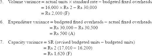
- Expenditure variance: It is that portion of fixed overhead variance that is due to difference between the budgeted fixed overheads and the actual fixed overheads incurred during a particular period. It is expressed as
Expenditure variance = budgeted fixed overhead – sactual fixed overheads
Expenditure variance = budgeted hours × standard fixed overhead rate per hour – actual fixed overheads
- Volume variance:
Volume variance = actual output × standard rate – budgeted fixed overheads or standard rate
(Actual output – budgeted output)or
Volume variance = standard rate per hour (standard hours produced – actual hours)
- Standard hours produced refers to the number of hours that should have been taken for the actual output as per the standard laid down. Volume variance can be further subdivided into three variances as follows:
- Capacity Variance:
Capacity variance = standard rate (revised budgeted units – budgeted units)
or
Capacity variance = standard rate (revised budgeted hours – budgeted hours)
- Calendar Variance:
Calendar variance = increase or decrease in production due to more or less working dayss at the rate of budgeted capacit × standard rate per unit
- Efficiency variance:
Efficiency variance = standard per unit (actual production[in units] – standard production[in units])
or
Efficiency variance = standard rate per hour (SH produced – AH)
- Capacity Variance:
Here, standard production or hours refers to budgeted production or hours adjusted to increase or decrease production due to capacity or calendar variance.
15.8 SALES VARIANCE
15.8.1 Profit method of calculating sales variances
The sales variances according to the profit method of calculating variances can be analysed as follows:
- Total sales margin variance (TSMV):
TMSV = actual profit – budgeted profit
or
TMSV = actual quantity of sales × actual profit per unit – budgeted quantity of sales × budgeted profit per unit
- Sales margin variance (SMnV):
SMnV = actual quantity of sales (actual selling price per unit – standard selling price per unit)
or
SMnV = standard profit per unit (actual quantity of sales – budgeted quantity of sales)
SMnV due to volume can be divided into two parts as follows:
- Sales margin variance due to sales mixture
- Sales margin variance due to sales quantities
15.8.1.1 SMnV Due to Sales Mixture
It is calculated as follows:
SMV due to sales mixture = standard profit per unit (AQ of sales – standard proportion for actual sales)
or
SMnV due to sales mixture = standard profit revised standard profit
15.8.1.2 SMV due to Sales Quantities
It is calculated as follows:
or
15.8.2 Value method of calculating sales variances
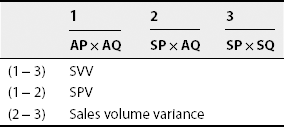
15.8.2.1 Sales Value Variance (SVV)
SVV arises due to one or more of the following reasons:
- Actual selling price is higher or lower than the SP. This is expressed in sales price variance.
- AQ of goods sold may be more or less than the budgeted quantity of sales. This is expressed in sales volume variance.
- Actual mix of various varieties sold may differ from the standard mix. This is expressed in sales mix variance.
- Revised standard sales quantity may be more or less than the budgeted quantity of sales. This is expressed in sales quantity variance.
15.8.2.2 Sales Price Variance (SPV)
15.8.2.3 Sales Volume Variance (S. Vol. V)
Sales volume variance can be divided into two parts as follows:
- Sales mix variance (SMxV):
Sales mix variance = standard value of actual mix – standard value of revised standard mix
- Sales quantity variance (SQV):
Sales quantity variance = standard selling price (revised standard sales quantity – budgeted sales quantity)
15.9 MATERIAL VARIANCES
Illustration 1
From the data given, calculate MPV, MUV and MMV:
Consumption per 100 units of product

Solution:
- MPV:
MPV =AQ (SR – AR)
Material A: 50 (Rs 50 – Rs 50) = Nil
B: 40 (Rs 40 – Rs 45) = Rs 200 Adverse
Rs 200 (A)
- MUV:
MUV =SR (SQ – AQ)
Material A: 50 (40 – 50) = 500 (Adverse)
B: 40 (Rs 50 – Rs 40) = 400 (Favorable)
100 (A)
- MMV: Here, the actual weight of mix and standard weight of mix differ from each other; therefore,
MMV = SR (RSQ – AQ)
- Here, the RSQ formula is as follows:
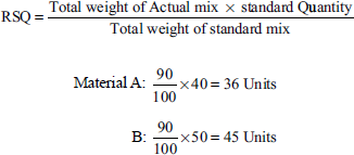
Then,
Material Mix variance = SR (RSQ – AQ)
Material A: 50 (36 – 50) = 700 Adverse
B: 40 (45 – 40) = 200 Favorable
500 (A)
Revised material usage variance = Standard Rate (SQ – RSQ)
Material A: 50 (40 – 36) = 200 Favorable
Material B: 40 (50 – 45) = 200 Favorable
400 (F)
MCV:
MCV = (SQ × SR) – (AQ × AR)
Material A: (40 × 50) – (50 × 50) = 500 (Adverse)
B: (50 × 40) – (40 × 45) = 200 (Favorable)
300 (A)
Illustration 2
A manufacturing concern, which has adopted standard costing, furnishes the following information:

Calculate (a) MUV, (b) MPV (c) MCV.
Solution:
SQ:
For 80–kg standard output,
SQ of material = 100 kg
SQ for 2,00,000 kg of finished products
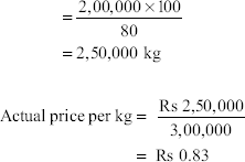
Illustration 3
From the following particulars, compute (a) MCV, (b) MPV and (c) MUV:
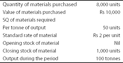
Solution:
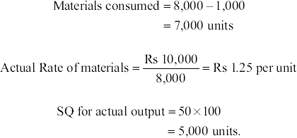
Illustration 4
From the following particulars, calculate (a) Total MCV, (b) MPV and (c) MUV:

Solution:
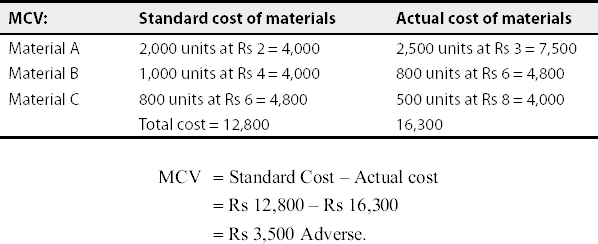
(b) MPV:
MPV = AQ (SR – AR)
Material A: 2,500 (Rs 2 – Rs 3) = 2,500 (A)
Material B: 800 (Rs 4 – Rs 6) = 1,600 (A)
Material C: 500 (Rs 6 – Rs 8) = 1,000 (A)
Total MPV = 5,100 (adverse)
(c) MUV:
MUV = SR (SQ – AQ)
Material A: Rs 2 (2,000 – 2,500) = 1,000 (A)
Material B: Rs 4 (1,000 – 800) = 800 (F)
Material C: Rs 6 (800 – 500) = 1,800 (F)
Total MUV = 1,600 (favourable)
Illustration 5
From the following information, find (a) price variance, (b) usage variance and (c) cost variance:
| SQ of sunmica per table | 5 sqft |
| SP per 5 sqft of sunmica | Rs 8.00 |
| Actual production of tables | 2,000 |
| Sunmica actually used | 4,500 sqft |
Solution: Actual purchase price of sunmica per square feet = Rs 6.00
- MPV:

- MUV:

- MCV:

Illustration 6
Standard mix for the production of X:
Material A: 50 tonnes at Rs 5 per tonne
Material B: 40 tonnes at Rs 15 per tonne
Actual mixture:
Material A: 100 tonnes at Rs 6 per tonne
Material B: 80 tonnes at Rs 7 per tonne
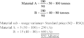
Calculate (a) MPV, (b) sub–usage variance and (c) mix variance.
Solution:
- material price variance = Actual quantity (Standard price – Actual price)
Material A = 100 (5 – 6) = 100 (A)
Material B = 80 (15 – 7) = 640 (F)
MPV = 540 F
-

-

Illustration 7
Standard mix of a product comprises the following:
X: 500 units at 15 paise per unit
Y: 1,000 units at 20 paise per unit
Z: 1,500 units at 25 paise per unit
Consumption was as follows:
X: 600 units at 30 paise per unit
Y: 800 units at 20 paise per unit
Z: 1,000 units at 15 paise per unit
Calculate material variance.
Solution:
Standard cost of standard materials:
X: 500 × Rs 0.15 = Rs 75
Y: 1000 × Rs 0.20 = Rs 200
Z:1500 × Rs 0.25 = Rs 375
3000 Rs 650
Actual cost of actual materials:
X: 600 × Rs 0.30 = 180
Y: 800 × Rs 0.20 = 160
Z: 1000 × Rs 0.15 = 150
2400 Rs 490
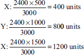
Revised quantity:
- MCV:

- MPV:
MPV = AQ (SP – AP)
X: 600 (0.15 – 0.30) = 600 (–0.15) = Rs 90 (Adverse)
Y: 800 (0.20 – 0.20) = Nil
C: 1000 (0.25 – 0.15) = 1000 (0.10) = Rs 100 (Favorable)
Rs 10 Favorable
- MUV = SP (SQ – AQ)
X: 0.15 (500 – 600) = 0.15 (–100) = Rs 15 (A)
Y: 0.20 (1000 – 800) = 0.20 (200) = Rs 40 (F)
Z: 0.25 (1500 – 1000) = 0.25 (500) = Rs 125 (F)
Rs 150 Favorable
- MMV: SP (RSQ – AQ)
X: 0.15 (400 – 600) = 0.15 (–200) = Rs 30 (A)
Y : 0.20 (800 – 800) = 0.20 (0) = Nil
Z : 0.25 (1200 – 1000) = 0.25 (200) = Rs 50 (F)
Rs 20 Favorable
Illustration 8
Standard cost of a certain chemical mixture is as follows:
40% material A at Rs 40 per tonne
60% material B at Rs 30 per tonne
A standard loss of 10% is expected in production.
Actual cost of materials used:
90 tonnes of material A at a cost of Rs 42 per tonne
160 tonnes of material B at a cost of Rs 28 per tonne
Actual output is 230 tonnes.
Calculate material variances.
Solution:
-

- MPV = AQ (SP – AP)
Material A = 90 (Rs 40 – Rs 42) = Rs 180 (A)
Material B = 160 (Rs 30 – Rs 28) = Rs 320 (F)
Rs 140 (F)
- MUV = SP (SQ – AQ)
Material A = Rs 40 (100/225 × 230 – 90) = Rs 489 (F)
Material B = Rs 30 (150/225 × 230 – 160) = Rs 200 (A)
Rs 289 (F)
- MMV = standard cost of standard mix – standard cost of actual mix
= Rs 8,500 – Rs 8,400
= Rs 100 (F)
-

Illustration 9
The standard cost of a chemical mixture is as follows:
8 tonnes of material A at Rs 40 per tonne
12 tonnes of material B at Rs 60 per tonne
Standard yield is 90% of input.
Actual cost for a period is as follows:
10 tonnes of material A at Rs 30 per tonne
20 tonnes of material B at Rs 68 per tonne
Actual yield is 26.5 tonnes. Calculate all material variances.
Solution:
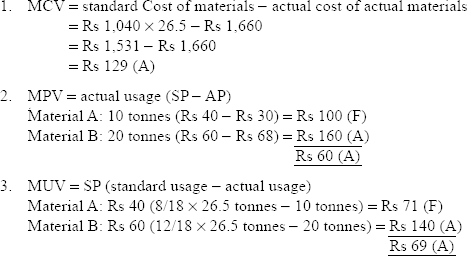

Illustration 10
The standard material cost for 100 kg of chemical D comprises
Chemical A: 30 kg at Rs 4 per kg
Chemical B: 40 kg at Rs 5 per kg
Chemical C: 80 kg at Rs 6 per kg
In a batch, 500 kg of chemical D were produced from a mix of
Chemical A: 140 kg at a cost of Rs 588
Chemical B: 220 kg at a cost of Rs 1,056
Chemical C: 440 kg at a cost of Rs 2,860
How do the yield, mix and the price factor contribute to the variance in the actual per 100 kg of chemical D over the standard cost?
Solution:
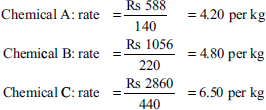
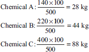
In chemical D of 500 kg, the chemical A is 140 kg.
Per 100 kg of chemical D, the required quantity is
- MCV:
MCA = (SQ × SP) – (AQ × AP)
Chemical A = (30 × Rs 4) – (28 × Rs 4.20) = Rs 2.40 (F)
Chemical B = (40 × Rs 5) – (44 × Rs 4.80) = Rs 11.20 (A)
Chemical C = (80 × Rs 6) – (88 × Rs 6.50) = Rs 92.00 (A)
Total MCA = Rs 100.80 (A)
- MPV:
MPV = AQ (SP – AP)
Chemical A = 28 (4 – 4.20) = Rs 5.60 (A)
Chemical B = 44 (5 – 4.80) = Rs 8.80 (F)
Chemical C = 88 (6 – 6.50) = Rs 44.00 (A)
Total MPV = Rs 40.80 (A)
- MUV:
MUV = SP (SQ – AQ)
Chemical A: 4 (30 – 28) = Rs 8 (F)
Chemical B: 5 (40 – 44) = Rs 20 (A)
Chemical C: 6 (80 – 88) = Rs 48 (A)
Total MUV = Rs 60 (A)
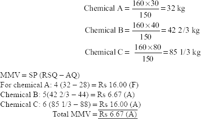
- MMV:
MMV = SP (RSQ – AQ)
The actual quantity is 160 kg, which is to be apportioned in the standard proportion, that is, 30:40:80.
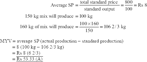
- MYV:
Illustration
A limited company produces an article by blending two basic raw materials. It operates a standard costing system and the following standards have been set for new materials:
| Material | Standard mix | SP per kilogram |
| A | 40% | Rs 5.00 |
| B | 60% | Rs 8.00 |
The standard loss in processing is 20%. During April 1994, the company produced 2,000 kg of finished output. The position of stocks and purchases for the month of April 1994 is as follows:
Material stock on 1 April 1994 (kg) Stock on 30 April 1994 (in kilogram) purchased during April 1994 Cost RS
Illustration 11
Calculate the following variances:
- MPVs
- MUVs
- MYV
- MMVs
Finished output is 2,000 kg. Standard loss in processing is 20%.
![]()
For an input of 2,500 kg, standard cost will be as follows:

Actual cost:


- MYV: SYR × (AY – SY)
= 5 (2,000 – 1,700) = 1,500
- MMV: SR (RSQ – AQ)
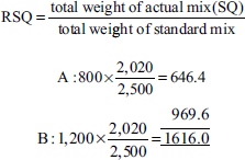
Illustration 12
The standard cost of a certain drug is 40% of material A at Rs 20 per pound. 60% of material B is Rs 30 per pound. Standard loss expected in production is 10%. In a certain period, 90 lb of material A at Rs 18 per pound and 110 lb of material B at Rs 34 per pound were used. Good production realized was 182 lb. Calculate the different material variances
Solution:
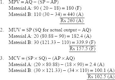
4. MYV = average SP (actual loss on actual output – standard loss on standard output)

Illustration 13
The standard cost of a chemical mixture is as follows:
8 tonnes of material A at Rs 40 per tonne
12 tonnes of material B at Rs 60 per tonne
Standard yield is 90% of input.
Actual cost for a period is as follows:
10 tonnes of material A at Rs 30 per tonne
20 tonnes of material B at Rs 68 per tonne
Actual yield is 26.5 tonnes.
Calculate all material variances.
Solution:
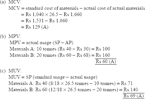
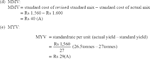
Illustration 14
With the help of following information, calculate
- LCV
- LRV
- LEV
Standard hours = 50 at Rs 5 per hour
Actual hours = 60 at Rs 6 per hour
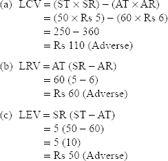
Illustration 15 Using the following information, calculate labour variances:
Gross direct wages = Rs 3,000
Standard hours produced = 1,600
Standard rate per hours = Rs 1.50
Actual hours paid are 1,500 hours, out of which hours not worked (abnormal idle time) are 50 hours
Solution:
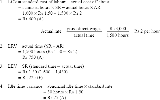
Illustration 16
A gang of workers usually consists of 10 men, 5 women and 5 boys in a factory. They are paid at standard hourly rates of Rs 1.25, Re 0.80 and Re 0.70, respectively. In a normal working week of 40 hours, the gang is expected to produce 1,000 units of output.
In a certain week, the gang consisted of 4 men and 3 boys. Actual wages were paid at the rates of Rs 1.20, Re 0.85 and Re 0.65, respectively. Two hours per work were lost due to abnormal idle time and 960 units of output were produced. Calculate various labour variances.
Solution:
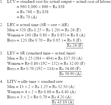

Illustration 17 The following is information related to the manufacturing process of a company:
Number of employees = 200
Weekly hours worked = 50
Standard wage rate = Re 1 per hour
Standard output = 250 units per hour
During the first week of February, four employees were paid Re 0.50 per hour and two employees Re 0.60 per hour, whereas the rest were paid standard rates. Idle time was 1 hour per employee. Actual output was 10,500 articles. Calculate labour variances.
Solution:
Actual cost of labour:
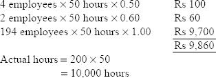
Idle time is 1 hour per employee. So, actual hours = 10,000 – 200 = 9,800
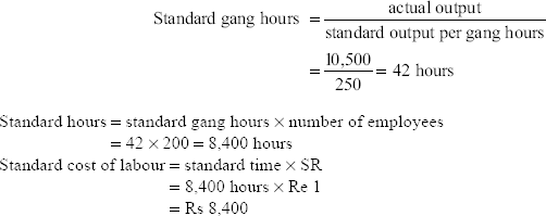
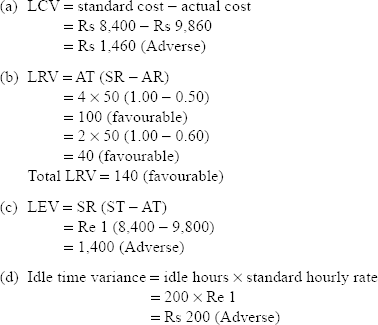
Illustration 18
Find out different labour variances with the following information:
| Standard | Actual | |
| Output | 1,000 units | 1,200 units |
| Rate of payment | Rs 6 per unit | Wages paid with a bonus of Rs 8,000 |
| Time taken | 50 hours | 40 hours |

Standard hours for 1,200 units actually produced:
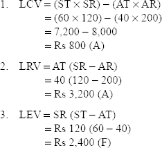
Illustration 19
Using the following information, calculate LCV, LRV, labour efficiency and idle time variance:
Standard hours: 6,000
Standard wage rate: Rs 5 per hour
Actual hours: 8,000
Actual wage rate: Rs 4 per hour
Time lost on account of breakdown of machinery = 300 hours
Solution:
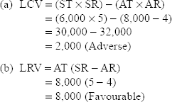

Illustration 20 Standard labour hours and rate for the production of Article A are given:
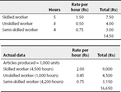
Calculate (a) LCV, (b) LRV, (c) LMV and (d) LYV.
Solution:
- LCV: (ST × SR) – (AT × AR)
Standard hours for actual production = actual units × ST
Skilled worker: 1,000 × 5 = 5,000 hours
Unskilled worker: 1,000 × 8 = 8,000 hours
Semi–skilled worker: 1,000 × 4 = 4,000 hours
LCV:
Skilled worker:(5,000 × Re 1.50) – (4,500 × Re 2)
= Rs 7,500 – Rs 9,000 = Rs 1,500 (A)
Unskilled worker: (8,000 × Re 0.50) – (1,000 × Re 0.45)
= 4,000 – 4,500
= Rs 500 (A)
Semi–skilled worker: (4,000 × Re 0.75) – (4,200 – Re 0.75)
= 3,000 – 3,150
= Rs 150 (A)
- LRV : AT (SR – AR)
Skilled worker: 4,500 (1.50 – 2) = Rs 2,250 (A)
Semi–skilled worker: 4,200 (0.75 – 0.75) = nil
Unskilled worker: 1,000 (0.50 – 0.45) = Rs 50 (F)
Total LRV = Rs –2,200 (A)
- (c) LMV: SR (RSQ) – actual mix
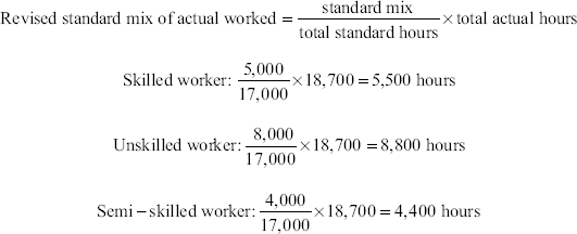
LMV:
Skilled worker: 1.50 (5,500 – 4,500) = Rs 1,500 (F)
Unskilled worker: 0.50 (8,800 – 10,000) = Rs 600 (A)
Semi–skilled worker: 0.75 (4,400 – 4,200) = Rs 150 (F)
Total LMV = Rs 1,050 (F)
- LYV: SR (SH for actual production – RSQ)
Skilled worker: 1.50 (5,000 – 5,500) = Rs 750 (A)
Unskilled worker: 0.50 (8,000 – 8,800) = Rs 400 (A)
Semi–skilled worker = 0.75 (4,000 – 4,400) = Rs 300 (A)
TLEV = Rs 1,450 (A)
Illustration 21
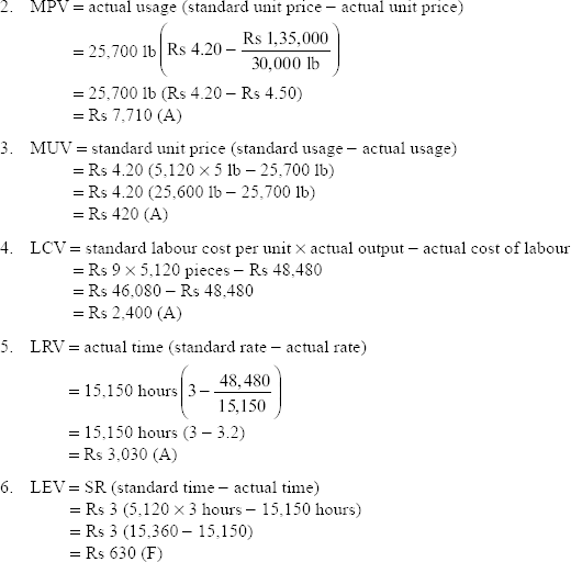
Tom Industries turns out only one article, the prime cost standards for which have been established as follows per completed piece
| Material—5 lb at Rs 4.20 | Rs 21 |
| Labour—3 hours at Rs 3 | Rs 9 |
The production schedule for July 2001 required the completion of 5,000 pieces. However, 5,120 pieces were actually completed. Purchases for the month of July 2001 amounted to 3,000 lb of material at the total invoice price of Rs 1,35,000. Production records for the month of July 2001 showed the following actual results:
Materials requisitioned and used = 25,700 lb
Direct labour: for 15,150 hours at Rs 48,480
Calculate appropriate material and labour variances.
Solution:

Overhead variance
Illustration 22
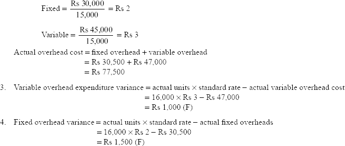
From the following data, calculate overhead variances:
| Budgeted | Actual | |
| Output | 15,000 units | 16,000 units |
| Number of working days | 25 | 27 |
| Fixed overheads | Rs 30,000 | Rs 30,500 |
| Variable overheads | Rs 4,500 | Rs 47,000 |
There was an increase of 5% in capacity.
Solution:

Sales variance
Illustration 23
A company is operating a system of standard costing and closing its books quarterly. The budgeted overheads were Rs 2,55,000. The overhead rate was predetermined at Rs 5 per labour hour, and during a period the company actually utilized 52,000 labour hours, whereas it should have spent only 51,000 hours. The actual overheads gave a rate of Rs 4.9 per labour hour. How would you record the variances?
Solution:
Standard overheads per labour hour = Rs 5.1
Standard time for actual production = 51,000 hours
Standard overheads for actual output = 51,000 × 5.1 = Rs 2,60,100
Actual overheads per labour hour = Rs 4.9
Actual time taken = 52,000 labour hours
Actual overheads = 52,000 × 4.9 = Rs 2,54,800


Illustration 24
From the following particulars, calculate all sales variances according to (A) profit method and (B) value method:

Solution:
(A) Profit method

- SMV due to selling price = AQ of sales (actual sales price per unit – budget sales price)

- SMVs due to volume = standard profit per unit (AQ of sales – budgeted quantity of sales)

- SMV due to sales mix = standard profit (AQ of sales – standard proportion for actual sales)

- SMV due to sales quantity = standard profit (standard proportion for actual sales – budgeted quantity of sales)

CHAPTER SUMMARY
After reading this chapter, one is able to understand the importance of standard costing in fixing the cost of a product, the concept of having favourable and unfavourable variances, the significance of having favourable variances in cases where yield is the main factor and the difficulty in setting standards.
KEY FORMULAE
Material Variances
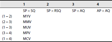
Note: SP = standard price
SQ = standard quantity
RSQ = revised standard quantity
AP = actual price
AQ = actual quantity
Column 2 is applicable only if there is a mixture of more than one raw material; otherwise, only the column 3 formula is enough, that is,
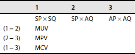
Note: RSQ = total AQ/total SQ × SQ for each item of material.
Sales Variances
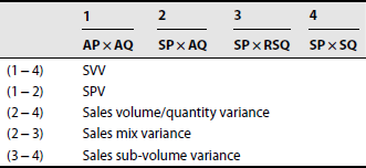
Note: Column 3 is not applicable if there is only one kind of product sold as follows:
Sales Margin Variances, that is, Profit Variances
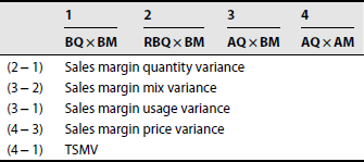
BQ = budgeted quantity
BM = budgeted margin
RBQ = revised budgeted quantity
AQ = actual quantity
AM = actual margin
Sales Price Variances
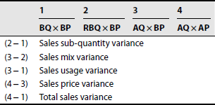
Note: AP = actual price
BP = budgeted price
Labour Variances
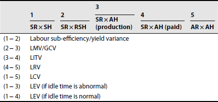
Note:
SR = standard rate
SH = standard hours
AH = actual hours
AR = actual rate
RSH = revised standard hours
Column 2 is not applicable if there is no mix of more than one kind of labour as follows:
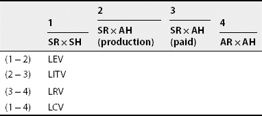
Overhead Variances
Variable overhead variances
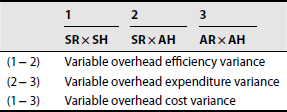
Note:
SR = standard rate
SH = standard hours
AR = actual rate
AH = actual hours
Fixed overhead variances
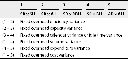
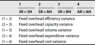
Note: RBH = revised budgeted hours
BH = budgeted hours
EXERCISE FOR YOUR PRACTICE
Objective-Type Questions
I. State whether the following statements are true or false
- Standards are fixed for each industry by trade unions.
- Standards are arrived at on the basis of past performance.
- Standards for material labour and overheads are interconnected.
- Variance means the difference between budget and standard costs.
- Standards do not allow any wastage.
- Yield variance shows the efficiency of labour.
- Standard cost is a historical cost.
- Standard costing is widely applied in process industries.
- Three types of standards are current, basic and normal.
- A set of standards provides yardsticks against which actual costs are compared.
[Ans: 1—false, 2—false, 3—true, 4—false, 5—false, 6—false, 7—false, 8—true, 9—true, 10—true]
II. Choose the correct answer
- Standard cost is a
- Predetermined cost
- Variable cost
- Fixed cost
- Profit
- Idle time variance = idle time ×
- Standard rate
- Actual rate
- Predetermined rate
- Loss
- Standard costing is more widely applied in
- Process industries
- Engineering industries
- Both (a) and (b)
- None of the above
- The technique of standard costing may not be applicable in the case of
- Large concerns
- Small concerns
- Transport
- Education
- LCV is the difference between standard cost of labour and
- Variable cost
- Fixed cost
- Actual cost of labour
- Marginal cost of labour
- Standard costing was developed because of the limitation of
- Job costing
- Marginal costing
- Labour costing
- Historical costing
- Management by exception is exercising control over
- Favourable items
- Unfavourable items
- Standard times
- Standard profit
- Standard cost of labour – actual cost of labour =
- Total cost variance
- Total labour cost
- Total material cost
- Idle time variance
- The deviation of actual cost or profit or sales from standard cost is known as
- Labour variance
- Variance
- Material variance
- Cost variance
- Material usage variance = material mix variance +
- Cost variance
- Labour variance
- MYV
- Fixed cost
[Ans: 1—(a), 2—(a), 3—(c), 4—(b), 5—(c), 6—(d), 7—(b), 8—(b), 9—(b), 10—(c)]
DISCUSSION QUESTIONS
- What is standard costing and how is it different from budgetary control?
- Variance analysis is an integral part of standard costing. Explain.
- What is variance? When is it called favourable and when is it called unfavourable?
- What is RSQ? When does it arise?
- Distinguish between ideal standard and normal standard.
- What are the limitations of standard costing?
- Discuss the factors involved in setting a standard for a product.
- Discuss the possibility of always having variances as favourable.
- Explain the importance of sales variance.
- Explain the factors to be kept in mind while determining overhead variance.
PROBLEMS
- From the following data, calculate MPV, MUV and MMV
Raw material Standard Actual A 40 units at Rs 50 per unit 50 units at Rs 50 per units B 60 units at Rs 40 per unit 60 units at Rs 45 per unit (I.C.W.A)
[Ans: MPV = Rs 300 (A); MUV = Rs 500 (A); MMV = Rs 60 (A)]
- Given that the cost standard for materials consumption is 40 kg at Rs 10 per kilogram, compute the variances when actuals are 48 kg at Rs 12 per kilogram.
[Ans: MCV = Rs 176 (A); MUV = Rs 80 (A); MPV = Rs 96
- From the following data, calculate MUV:
Standard: 10 kg at Rs 4 per kilogram
Actual: 12 kg at Rs 4.50 per kilogram
(B. Com., Madurai)
[Ans: MCV: Rs 14 (A); MUV: Rs 8 (A)]
- The standard material required to manufacture one unit of product A is 5 kg and the SP per kilogram of material is Rs 3. The cost accountant's records, however, reveal that 16,000 kg of material costing Rs 52,000 were used for producing 3,000 units of product A. Calculate the variances.
[Ans: MCV = Rs 7,000 (adverse); MUV = Rs 3,000 (adverse); MPV = Rs 4,000 (adverse)]
- Gemini Industries provide the following information from their records: For making 10 kg of GEMCO, the standard requirement is as follows:
Quantity (kg) Rate per kilogram (Rs) Material A 8 6.00 Material B 4 4.00 During April, 100 kg of GEMCO were produced. The actual consumption of material is as follows:
Quantity (kg) Rate per kilogram (Rs) Material A 750 7.00 Material B 500 8.00 Calculate (a) MCV, (b) MPV and (c) MUV.
(C.A. Inter)
[Ans: MPV = Rs 1,250 (A); MCV = Rs 1,350 (A); MUV = Rs 100 (A)]
- Calculate MPV, MUV and MCV from the following information:
Quantity of materials purchased 3,000 units Value of materials purchased Rs 14,000 SQ of material required per tonne of finished product 20 units SP of material Rs 5 per unit Opening stock of materials 100 units Closing stock of materials 600 units Finished product manufactured 100 tonnes [Ans: MPV = Rs 800 (favourable); MUV = Rs 2,500 (adverse); MCV = Rs 1,700 (adverse)]
- From the particulars given, calculate the following material variances and give their relationships:
(1) MCV, (2) MUV, (3) MPV, (4) MMV and (5) material sub-usage variance


[Ans: MCV = Rs 12 (A); MPV = Rs 6 (F); MUV = Rs 18 (A); MMV = Rs 2 (A); MSUV = Rs 16 (A)]
Labour Variances
- Calculate LCVs for the following information:
Standard hours: 40 at Rs 3 per hour
Actual hours: 50 at Rs 4 per hour
(B.Com., Calicut; B.Com., Madurai; B.Com., Rajasthan)
[Ans: LCV = Rs 80 (A); LRV = Rs 50 (A); LRV = Rs 30(A)]
- Data relating to a job are as follows:
Standard rate of wages per hour Rs 10 Standard hours 300 Actual rate of wages per hour Rs 12 Actual hours 200 [Ans: (i) Rs 600 (favourable); (ii) Rs 400 (adverse); (iii) Rs 1,000 (favourable)]
- In a factory section, there are 80 workers and the average rate of wages per worker is Re 0.50 per hour. Standard working hours per week are 45 hours and the standard performance is 6 units per hour. During the four weeks of February, wages paid for 40 workers were Re 0.50 per hour, for 15 workers Re 0.60 per hour and for 25 workers Re 0.40 per hour. The section did not work for 4 hours due to breakdown of machinery. Work out the LRV for the section for 4 weeks.
[Ans: LRV = Rs 180 (favourable)]
- Calculate variances from the standard for a particular month as disclosed from the following figures:
Standard In a particular month Number of workers employed 600 550 Average wages per worker per month Rs 250 Rs 264 Number of working days in a month 25 24 Output in units 30,000 28,000 [Ans: LCV = Rs 5,200 (adverse); rate of pay variance = Rs 13,200 (adverse); efficiency variance = Rs 8,000 (favourable)]
Hint: Standard time for standard output of 30,000 units = 600 × 25 man days.
Standard time for actual output of

- A gang of workers normally consist of 30 men, 15 women and 10 boys. They are paid at standard hourly rates as follows:
Re Men 0.80 Women 0.60 Boys 0.40 In a normal working week of 40 hours, the gang is expected to produce 2,000 units of output. During the week ending on 31 December 1997, the gang consisted of 40 men, 10 women and 5 boys. For these workers, the actual wages paid were Re 0.70, Re 0.65 and Re 0.30, respectively. Four hours per week were lost due to abnormal idle time and 1,600 units were produced. Calculate all labour variances.
[Ans: LCV = Rs 256 (A); LRV = Rs 160 (F); TLEV = Rs 416 (A); ITV = Rs 160 (A); LEV = Rs 256 (A); LMV = Rs 108 (A); LYV = Rs 148 (A)]
- Following data are available from a record of a factory:
Standard labour rate Rs 2 per hour Standard hours 2 per unit Actual labour rate Rs 2.25 per hour Actual units produced 1,000 units Actual hours worked 1,950 hours Calculate labour variances.
(B.Com.)
[Ans: LRV = Rs 487.50 (A); LEV = Rs 100.00 (F); LCV = Rs 387.50 (A)]
- Data relating to a job are as follows:
Standard rate of wages per hour = Rs 10
Standard hours 300 Actual rate of wages per hour Rs 12 Actual hours 200 You are required to calculate (i) LCV, (ii) LRV and (iii) LEV.
(B. Com. Honours, Delhi)
[Ans: LCV = Rs 600 (F); LRV = Rs 400 (A); LEV = Rs 1,000 (F)]
Overhead Variances
- A factory has estimated its overheads for a year at Rs 96,000. The factory runs for 300 days in a year; it works 8 hours a day. The total budgeted production for the year is 24,000 articles. Actual data are also given as follows for the month of April 1994:
Actual overhead Rs 8,500 Output 2,100 articles Idle time 4 hours Calculate: (1) overhead cost variance, (2) overhead budget variance, (3) overhead efficiency variance and (4) idle time variance.
[Ans: OCV = Rs 100 (A); OEV = Rs 500 (A); OEV = Rs 560 (F); ITV = Rs 160 (A)]
-
Items Budget Actual Number of working days 20 22 Manhours per day 8,000 8,400 Output per manhour in units 1.00 0.90 Overhead cost 1,60,000 1,68,000 From the aforementioned data, calculate overhead variances such as (i) overhead cost variance, (ii) overhead efficiency variance, (iii) overhead capacity variance and (iv) overhead calendar variance.
(C.A.)
[Ans: (i) Rs 1,680 (A); (ii) Rs 18,480 (A); (iii) Rs 24,800 (F); (iv) Rs 16,000 (F)]
- Calculate overhead variances from the following data:
Standard Actual Fixed overheads (Rs) 8,000 8,500 Variable overheads (Rs) 12,000 11,200 Output in units 4,000 3,800 [Ans: overhead cost variance = Rs 700 (adverse); variable overhead variance = Rs 200 (favourable); fixed overhead variance = Rs 900 (adverse); volume variance = Rs 400 (adverse); fixed overhead expenditure variance = Rs 500 (adverse)]
- A manufacturer operating a standard costing system has the following data for a month:
Standard Actual Number of working days 25 27 Manhours per month 5,000 5,400 Output in units 500 525 Fixed overheads (Rs) 2,500 2,400 Calculate fixed overhead variances for the month.
[Ans: total fixed overhead variance = Rs 225 (favourable); volume variance = Rs 125 (favourable); expense variance = Rs 100 (favourable); capacity variance = nil; calendar variance = Rs 200 (favourable); efficiency variance = Rs 75 (adverse)]
- Actual overhead: Rs 1,800
Budgeted overhead: Rs 2,000
Budgeted period: 4,000 labour hours
Standard per unit: 10 labour hours
Budgeted number of days: 20
Standard overhead per hour: Re 0.50
Actual number of days: 22
Actual hours: 4,300
Actual production: 425 units
Calculate (a) expenditure variance, (b) calendar variance, (c) capacity variance, (d) efficiency variance, (e) total overhead variance and (f) volume variance.
[Ans: expenditure variance = Rs 200 (F); calendar variance = Rs 200 (F); capacity variance = Rs 50 (A); efficiency variance = Rs 25 (A); volume variance = Rs 125 (F); total variance = Rs 325 (F)]
Sales variance
- The sales manager of a company engaged in the manufacture and sale of three products P, Q and R gives the following information for the month of October 1994:

Actual sales:
P 1,500 units for Rs 15,000 Q 2,500 units for Rs 17,500 R 3,500 units for Rs 21,000 - You are required to calculate the following variances:
- Sales price variance
- Sales volume variance
- Sales quantity variance
- Sales mix variance
- The cost of examining the cause of variances requires Rs 200 and the corrective action to be taken, if needed, requires Rs 300. If there is 85% probability of the variances arising out of justifiable reasons and 15% probability of the situation going completely out of control, work out the total cost in carrying out a complete investigation.
(C.A. Final)
[Ans: SPV = Rs 2,000 (A); SVV = Rs 5,500 (F); SQV = Rs 12,500 (F); SMV = Rs 7,000 (A)]
- You are required to calculate the following variances:
- From the following particulars, calculate (a) SVV, (b) SPV and (c) Sales volume variance. The budgeted and actual sales for a period in respect of two products are as follows:

(B.Com., Madurai)
[Ans: SVV = Rs 9,500 (F); SPV = Rs 1,000 (A); SVOV = Rs 10,500 (F)]
- From the following data, calculate (a) sales price variance, (b) sales volume variance and (c) sales mix variance:

[Ans: (a) Rs 2,000 (unfavourable); (b) nil; and (c) Rs 7,600 (unfavourable)]
- The following table shows the budgeted and actual sales for a certain period. Compute (a) price, (b) volume and (c) mix variance of sales from the following data:

Calculate SPV and SVV.
[Ans: (a) Rs 27,000 (favourable); (b) Rs 18,000 (favourable); (c) Rs 8,666.67 (favourable)]
- From the following budgeted and actual figures, calculate the variances on sales margin basis:
Budget Sales—2,000 units at Rs 15 each Rs 30,000 Cost of sales at Rs 12 each Rs 24,000 Profit Rs 6,000 Actual: Sales—1,900 units at Rs 14 each Rs 26,600 Cost of sales at Rs 10 each Rs 19,000 Profit Rs 7,600 (I.C.W.A.)
[Ans: Sales margin price variance = Rs 1,900 (F); sales margin quantity variance = Rs 300 (A); TSMV = Rs 1,600 (F)]
- Modern Toys Ltd had the following budgeted sales and actual sales from March 1998:

Calculate sales variances according to profit method.
[Ans: TSMV = Rs 5,050 (F); SMV due to selling price = Rs 4,800 (F);
SMV due to volume = Rs 250 (F); SMV due to
 ;
;SMV due to sales quantity


